3-D visualisation of palaeoseismic trench stratigraphy and trench logging using terrestrial remote sensing and GPR – combining techniques towards an objective multiparametric interpretation

(1)

SED

7, 2697–2733, 2015

An objective multiparametric interpretation of palaeoseismic trench

stratigraphy

S. Schneiderwind et al.

Title Page

Abstract Introduction

Conclusions References

Tables Figures

◭ ◮

Back Close

Full Screen / Esc

Printer-friendly Version

Interactive Discussion

Discussion

P

a

per

|

Discussion

P

a

per

|

Discussion

P

a

per

|

Discussion

P

a

per

|

Solid Earth Discuss., 7, 2697–2733, 2015 www.solid-earth-discuss.net/7/2697/2015/ doi:10.5194/sed-7-2697-2015

This discussion paper is/has been under review for the journal Solid Earth (SE). Please refer to the corresponding final paper in SE if available.

3-D visualisation of palaeoseismic trench

stratigraphy and trench logging using

terrestrial remote sensing and GPR –

combining techniques towards an

objective multiparametric interpretation

S. Schneiderwind1, J. Mason1, T. Wiatr2, I. Papanikolaou3, and K. Reicherter1

1

Institute of Neotectonics and Natural Hazards, RWTH Aachen University, Lochnerstraße 4–20, 52056 Aachen, Germany

2

Fundamental matters/Division GI, Federal Agency for Cartography and Geodesy, Richard-Strauss-Allee 11, 60598 Frankfurt am Main, Germany

3

Laboratory Mineralogy – Geology, Agricultural University of Athens, Iera Odos 75, Athens, 11855 Greece

Received: 24 August 2015 – Accepted: 30 August 2015 – Published: 22 September 2015

Correspondence to: S. Schneiderwind ([email protected])

(2)

SED

7, 2697–2733, 2015

stratigraphy

Title Page

Tables Figures

◭ ◮

Back Close

Full Screen / Esc

Discussion

P

a

per

|

Discussion

P

a

per

|

Discussion

P

a

per

|

Discussion

P

a

per

|

Abstract

Two normal faults on the Island of Crete and mainland Greece were studied to create and test an innovative workflow to make palaeoseismic trench logging more objec-tive, and visualise the sedimentary architecture within the trench wall in 3-D. This is achieved by combining classical palaeoseismic trenching techniques with

multispec-5

tral approaches. A conventional trench log was firstly compared to results of iso clus-ter analysis of a true colour photomosaic representing the spectrum of visible light. Passive data collection disadvantages (e.g. illumination) were addressed by comple-menting the dataset with active near-infrared backscatter signal image from t-LiDAR measurements. The multispectral analysis shows that distinct layers can be identified

10

and it compares well with the conventional trench log. According to this, a distinction of adjacent stratigraphic units was enabled by their particular multispectral composition signature. Based on the trench log, a 3-D-interpretation of GPR data collected on the vertical trench wall was then possible. This is highly beneficial for measuring repre-sentative layer thicknesses, displacements and geometries at depth within the trench

15

wall. Thus, misinterpretation due to cutting effects is minimised. Sedimentary feature

geometries related to earthquake magnitude can be used to improve the accuracy of seismic hazard assessments. Therefore, this manuscript combines multiparametric ap-proaches and shows: (i) how a 3-D visualisation of palaeoseismic trench stratigraphy and logging can be accomplished by combining t-LiDAR and GRP techniques, and (ii)

20

how a multispectral digital analysis can offer additional advantages and a higher

ob-jectivity in the interpretation of palaeoseismic and stratigraphic information. The multi-spectral datasets are stored allowing unbiased input for future (re-)investigations.

1 Introduction

Seismic hazard assessment is still predominantly based on the instrumental and

histor-25

(3)

com-SED

7, 2697–2733, 2015

stratigraphy

Title Page

Tables Figures

◭ ◮

Back Close

Full Screen / Esc

Discussion

P

a

per

|

Discussion

P

a

per

|

Discussion

P

a

per

|

Discussion

P

a

per

|

pared to the recurrence interval of particular faults (e.g. Wesnousky, 1986; Yeats and Prentice, 1996; Machette, 2000). As a result, the sample from the statistical elabora-tion of the historical and instrumental data is incomplete and a large number of faults would have not ruptured during the period where the historical record is considered complete (Grützner et al., 2013; Papanikolaou et al., 2015). The need for fault specific

5

studies and the extraction of recurrence intervals from palaeoseismological trenches was then initiated in the late 1970s (Sieh, 1978; McCalpin, 2009). The goal is to extend the history of slip on a fault back many thousands of years, a time span that generally encompasses a large number of earthquake cycles (Yeats and Prentice, 1996).

Over the last few years fault specific studies and palaeoseismology have been

fur-10

ther advanced and are now supported by new remote sensing tools that o_ffer high

spatial resolution (e.g. LiDAR) and geophysics that extend our data into the subsurface (Ground Penetration Radar (GPR), Electric Resistivity Tomography (ERT)) (Papaniko-laou et al., 2015). This manuscript adds on such approaches and shows: (i) how a 3-D visualisation of palaeoseismic trench stratigraphy and logging can be accomplished by

15

combining t-LiDAR and GRP techniques, and (ii) how a multispectral digital analysis can o_ffer additional advantages and a higher objectivity in the interpretation.

Palaeoseismological studies are often undertaken to identify earthquake recurrence intervals and maximum credible magnitudes of prehistoric earthquakes (McCalpin, 2009). These parameters are needed for the accurate calculation of seismic hazard

20

potential of active fault zones (Michetti et al., 2005; Reicherter et al., 2009). Evidence for palaeoearthquakes can be found within the sedimentary architecture of active faults where conditions are favourable for their preservation. Typical features caused by re-current seismic events include: (i) progressive displacements (Keller and Rockwell, 1984), (ii) colluvial wedges, (iii) Liquefaction, and (iv) fissure fills (Reicherter et al.,

25

(4)

SED

7, 2697–2733, 2015

stratigraphy

Title Page

Tables Figures

◭ ◮

Back Close

Full Screen / Esc

Discussion

P

a

per

|

Discussion

P

a

per

|

Discussion

P

a

per

|

Discussion

P

a

per

|

potential archives of seismic information expensive trenches are excavated across de-formation zones. Then, the classical approach is to document stratigraphy and struc-ture by careful logging, either on paper and/or with photographs (e.g. Wallace, 1986; McCalpin, 2009). The accuracy of the trench log is, however, dependent on the logger’s experience and ability to define mappable units; discrete deposits that are composed

5

of similar lithology need to be distinguished from adjacent deposits.

Palaeoseismic indicators are widely spread and their formation varies along fault strike (e.g. Bubeck et al., 2015). For this reason, geophysical surveys undertaken prior to the trenching phase have become common practice over the last decade. For in-stance, ground-penetrating radar (GPR) measurements have been carried out to

iden-10

tify optimum trenching locations (e.g. Demanet et al., 2001; Alasset and Meghraoui, 2005; Grützner et al., 2012) and many studies have shown that earthquake related structures can be identified in the shallow subsurface with geophysics (e.g. Chow et al., 2001; Reiss et al., 2003; Bubeck et al., 2015). The excavated trench is then a 2-D rep-resentation of the fault zone stratigraphy. It is assumed that the 2-D geometry of the

15

logged sedimentary features continues along strike either side of case; without widen-ing the trench along strike, or excavatwiden-ing more trenches, we must assume that the 2-D trench log is representative for this location along the fault. Trenches target predomi-nantly palaeosols on either side of the fault, and then according to empirical relation-ships (Wells and Coppersmith, 1994) palaeomagnitudes can be estimated based on

20

these co-seismic displacements. If no or only poorly expressed displaced palaeosols exist the geometry of sedimentary features within trenches is used to estimate previous earthquake displacements. As a “rule of thumb” colluvial wedge thickness equals half of the initial scarp height (e.g. Reicherter, 2001; Reiss et al., 2003; McCalpin, 2009). Such information are then used as input parameters for seismic hazard assessment.

There-25

(5)

SED

7, 2697–2733, 2015

stratigraphy

Title Page

Tables Figures

◭ ◮

Back Close

Full Screen / Esc

Discussion

P

a

per

|

Discussion

P

a

per

|

Discussion

P

a

per

|

Discussion

P

a

per

|

In this study we demonstrate how high-resolution t-LiDAR (terrestrial light detection and ranging) measurements and photomosaics can be used to assist in the interpre-tation of palaeoseismological exposures; we also show how GPR can be used to vi-sualise sedimentary structures in 3-D within the trench wall. The t-LiDAR’s backscatter signal represents material reflectance of radiation in the near-infrared wavelength, and

5

digital photo cameras collect information of the reflectance of visible light; therefore, a quasi-multispectral inspection of the exposures is possible. Ragona et al. (2006) developed a method using imaging spectroscopy on palaeoseismic exposures with hy-perspectral and normal digital cameras. As an outcome they were able to enhance the visualisation of the sedimentary layers and other features that are not obvious or even

10

not visible to the human eye. Another study undertaken by Wiatr et al. (2015) places emphasis on the use of the monochromatic laser beam’s backscattered signal to deter-mine varying surface conditions. Using these techniques we make experienced-based trench logging more objective. GPR undertaken on top of the trench and on the ver-tical trench wall is used in combination with a high-resolution digital elevation model

15

(DEM) from t-LiDAR scanning. This allows radar facies (Neal, 2004) to be distinguished and the sedimentological architecture at depth within the trench wall to be identified. Thus, the resulting 3-D model from the GPR provides information on varying layer

thicknesses and minimises misinterpretation due to cutting effects. The workflow

com-prising data acquisition, statistical analysis, interpretation and storage was calibrated

20

on a road cut on the Island of Crete. We then applied this workflow on a professionally excavated trench in mainland Greece.

2 Geological setting of the study sites

The study sites are both located in Greece, which is one of the most seismically ac-tive parts of the Mediterranean (McKenzie, 1972; Le Pichon and Angelier, 1979;

Pa-25

(6)

SED

7, 2697–2733, 2015

stratigraphy

Title Page

Tables Figures

◭ ◮

Back Close

Full Screen / Esc

Discussion

P

a

per

|

Discussion

P

a

per

|

Discussion

P

a

per

|

Discussion

P

a

per

|

Papanikolaou, 1981; Lyon-Caen et al., 1988) has led to the development of bedrock fault scarps throughout both mainland Greece (Stewart and Hancock, 1991; Benedetti et al., 2002) and the island of Crete (e.g. Wiatr et al., 2013). These normal faults mainly consist of footwall Mesozoic carbonates juxtaposed against hanging-wall flysch and/or post-alpine sediments. Earthquake features such as colluvial wedges (a consequence

5

of degradation of the scarp), fissure fills and displaced strata occur within the hanging-walls of these faults and datable material may be contained within buried palaeosols (see Fig. 1vi) (McCalpin, 2009). To create those archives and preserve them over geo-logical timescales, erosional processes must be lower than the rate of tectonic activity. These features therefore represent geological archives of palaeoearthquakes because

10

they can record information about Holocene and Late Pleistocene earthquakes (e.g. Morey and Schuster, 1999; McCalpin, 2009). Ambraseys and Jackson (1990) estimate

a maximum earthquake magnitude ofM_s7.0 could occur on these normal faults, which

coincides with fault segment lengths of 15–30 km as determined through empirical re-lationships (Wells and Coppersmith, 1994).

15

2.1 The Sfaka Fault (NE Crete, Greece)

The island of Crete is the largest within the Greek territory and is directly adjacent to the subduction zone between Europe and Africa. The NNE–SSW trending Sfaka fault is located in northeastern Crete (Fig. 1i) and forms the easternmost segment within the Ierapetra Fault Zone which is a major tectonic line of approximately 25 km

20

cutting through the whole island (Gaki-Papanastassiou et al., 2009). This northwest

dipping normal fault is easy to recognise as it offsets smooth mountain slopes, has

a steeply dipping (ca. 70◦) fault scarp up to 6 m in height, and has an onshore length

of approximately 5 km (Fig. 1iv). Together with the opposing Lastros fault a 2 km wide graben structure is formed.

25

(7)

hanging-SED

7, 2697–2733, 2015

stratigraphy

Title Page

Tables Figures

◭ ◮

Back Close

Full Screen / Esc

Discussion

P

a

per

|

Discussion

P

a

per

|

Discussion

P

a

per

|

Discussion

P

a

per

|

wall colluvium (Fig. 1v). The outcrop cuts the fault at an angle of approximately 75◦

from the fault strike.

2.2 The Kaparelli Fault (Gulf of Corinth, Greece)

The Kaparelli fault is located in the easternmost part of the Gulf of Corinth (see Fig. 1i) which is associated with rapid extension oriented N-S (e.g. Papanikolaou and

Roy-5

den, 2007). The Kaparelli fault became well-known as it ruptured during the Corinthian Alkyonides earthquake sequence in spring 1981 (Jackson et al., 1982). Many palaeo-seismological studies using various approaches have been undertaken along this ca. 20 km long south dipping normal fault. For example Benedetti et al. (2003) used 36Cl cosmic ray exposure dating to determine the history of surface rupturing events on the

10

4–5 m high limestone scarp of the Kaparelli fault. Their results show evidence for

seis-mic activity 20±3, 14.5±0.5 and 10.5±0.5 ka prior to the 1981 earthquake sequence.

A palaeoseismological trenching study was conducted by Kokkalas et al. (2007). The

authors found evidence for at least three events in the past 10 000 years: 9370±120,

7290±140 and 1165±105 a. The excavations from Kokkalas et al. (2007) are still open;

15

therefore, the already logged and interpreted structures within trench Kap-1 (Fig. 1v) is a perfect site to test the workflow developed on the Sfaka fault road cut.

3 Methodology

The herein presented workflow combines palaeoseismic trenching techniques with t-LiDAR measurements to improve the accuracy of palaeoearthquake reconstruction.

20

(8)

SED

7, 2697–2733, 2015

stratigraphy

Title Page

Tables Figures

◭ ◮

Back Close

Full Screen / Esc

Discussion

P

a

per

|

Discussion

P

a

per

|

Discussion

P

a

per

|

Discussion

P

a

per

|

3.1 Palaeoseismic trenching

A palaeoseismic trench is characterised by an often artificially produced subsurface ex-posure of sedimentological coseismic features. To accurately interpret these features, apparent dips and anthropogenic and/or exogenous influences must be excluded. Moreover, sketching lithological contents requires an exposure devoid of weathered

5

and smeared parts that were caused by the excavation (McCalpin, 2009). To simplify and prove the geometrical correctness of the trench log, a reference grid of one square metre was attached to the wall. The grid’s points of intersection also act as reference points for remote sensing applications.

The trenches were conventionally logged in 1 : 10 scale in accordance with McCalpin

10

(2009). Thereby, discrete deposits that are composed of similar lithology considering consistent texture, sorting, bedding, fabric, and colour of individual layers are mapped. Photographs of every square metre were taken and later stitched together using an automatic panorama recognising tool including a manual editor of control points and straightening functions (Autopano Giga, Kolor). It must be noted that error values are

15

already stored within image information due to differing luminous exposures;

further-more, holes and protruding boulders create shadows that partially change the reflec-tion characteristics of certain sedimentological features. The Sfaka road cut faces north (see Fig. 1iv and v) and is surrounded by steep slopes. In Kaparelli the eastern trench wall (see Fig. 1ii and iii) was investigated because it preserved the best stratigraphy

20

and exhibits faulting events with clear marker horizon displacements (Kokkalas et al.,

2007). To avoid most of the differing luminous exposures, the photographs were either

taken in the morning when the angle of sunlight was shallow and did not shine directly onto the investigated wall (Kaparelli) or in the afternoon when the sun disappeared behind the surrounding hills (Sfaka).

25

The photomosaic of true colour images (RGB; red, green, blue) was converted into a grey-level image to eliminate hue and saturation information while retaining the

(9)

im-SED

7, 2697–2733, 2015

stratigraphy

Title Page

Tables Figures

◭ ◮

Back Close

Full Screen / Esc

Discussion

P

a

per

|

Discussion

P

a

per

|

Discussion

P

a

per

|

Discussion

P

a

per

|

age was georeferenced to a custom frame in order to make it comparable to all other datasets of this study.

3.2 t-LiDAR measurements

t-LiDAR (terrestrial Light Detection and Ranging) is a remote sensing technique with high spatial and temporal resolution and is a very effective instrument for

reconstruct-5

ing morphological and geological settings and monitoring approaches. A generated

coherent laser beam with little divergence by stimulated emission is reflected off

sur-faces and the proportionate backscattered signal is detected, forming a non-contact and non-penetrative active and stationary recording system. Thus, from measuring the two-way-travel time (TWT) of a first pulse detection sequence, 3-D surface data is

10

acquired. The illuminated area is controlled by wavelength, beam divergence, range between sensor and target, and also by the angle of incidence (Jörg et al., 2006; Wiatr

et al., 2015). In our study we used an ILRIS 3-D laser ranging system (wavelengthλis

1500 nm) from OPTECH Inc., Ontario, Canada.

The limitations of using t-LiDAR are high humidity (e.g. Lobell and Asner, 2002) and

15

low target reflection with cumulative distance and shallow incident angle (e.g. Höfle and Pfeifer, 2007). In order to assume constant soil moisture and to ensure the backscatter signal data quality, close range scans were done during the summer in dry conditions within a few hours. The scans were carried out almost perpendicular to the trench wall and less than 10 m from the exposure.

20

Other benefits of applying t-LiDAR is its flexibility, the relatively quick availability of an actual dataset, and also its high spatial resolution with information about backscatter signal each referenced inx,y,zcoordinates. The result is an irregular but dense point cloud representing a highly detailed digital 3-D surface model which can be easily implemented in geographical information systems (GIS) to generate accurate digital

25

(10)

SED

7, 2697–2733, 2015

stratigraphy

Title Page

Tables Figures

◭ ◮

Back Close

Full Screen / Esc

Discussion

P

a

per

|

Discussion

P

a

per

|

Discussion

P

a

per

|

Discussion

P

a

per

|

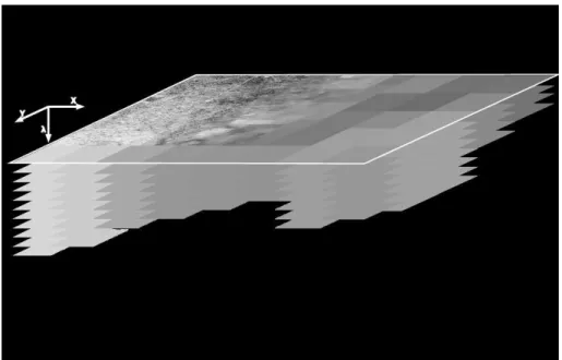
prolongation of the scarp, and trench wall (see Fig. 2). The backscatter signal of the t-LiDAR results from the reflection of transmitted waves of near-infrared light. In other words, each measurement is usually accompanied by a surface remission value, which quantifies the intensity of the reflected laser beam. The monochromatic backscat-ter signal values are stored as grayscale values from 0–255. The information on the

5

monochromatic wavelength and the detected backscattered signal in the near-infrared reflects the surface properties which are invisible to human eyes. Thus, the backscatter signal was also used for the multispectral analysis. The raw-data was cleaned from iso-lated points and those that do not represent the area of interest. The mathematical and

geometrical alignment of the different scan windows was then carried out. For project

10

specific demands, the datasets were translated into a custom grid. The long-mid range data were used for the overall geometrical analysis creating high-resolution DEMs with a resolution smaller than 0.1 m. Data from the close range scan were processed for sta-tistical calculations of the backscatter signal’s spatial distribution. A detailed description on the applied workflow is given in Sect. 3.3.

15

3.3 Imaging spectroscopy

Visualising an array of simultaneously acquired images that record separate wave-length intervals or bands is part of multispectral analyses. A common multispectral camera employs a range of film and filter combinations to acquire photographs that record narrow spectral bands of non-imaging data. Reflectance spectra map the

per-20

centage of incident energy (e.g. sunlight) that is reflected by a material as a function of energy wavelength. Absorption of incident energy is represented by downward ex-cursions of a curve (absorption features). Upward exex-cursions represent superior re-flectance (rere-flectance peaks). These features are valuable clues for recognising and distinguishing certain materials (Sabins, 1996). Multispectral imaging, or imaging

spec-25

troscopy, has been used at many different scales for remote sensing. Probably the most

(11)

SED

7, 2697–2733, 2015

stratigraphy

Title Page

Tables Figures

◭ ◮

Back Close

Full Screen / Esc

Discussion

P

a

per

|

Discussion

P

a

per

|

Discussion

P

a

per

|

Discussion

P

a

per

|

De Rose et al., 2011; Nouri et al., 2014). Ragona et al. (2006) introduced an appli-cation of high-resolution field imaging spectroscopy on paleoseismic exposures using hyperspectral and common digital photo cameras. The authors conclude that imaging spectroscopy can be successfully applied to assist in the description and interpreta-tion of palaeoseismic exposures because: (i) subtle or invisible features are displayed,

5

(ii) quantitative analysis and comparisons of units using reflectance spectra can be undertaken, and (iii) unbiased data are stored for future access and analysis.

The limitations of multispectral approaches are, by their very nature, closely con-nected to the application of photomosaics and t-LiDAR measurements. We re-emphasise the influence of moisture; where present it not only causes a darkening

10

of the sediments (reduction in reflectance), but there is also a hard-to-quantify content variation across the exposure (Ragona et al., 2006). Another error source appears due to morphological characteristics of a certain exposure, especially on surfaces that are not well prepared for palaeoseismic investigations and data collection. This means that the exposure must be flattened and cleaned to avoid changes in spectral amplitudes

15

accompanying changes in illumination angle and distance.

To reduce errors we assume that the moisture content was similar throughout the

exposure and water absorptions should not affect the correlations because the spectral

change is similar along the trench wall. Furthermore, the photos and t-LiDAR scans were taken almost perpendicular to the exposure so that optimal data quality can be

20

expected.

The workflow contains geo-referencing and snapping the high-resolution raster data from the photomosaic and t-LiDAR backscatter signal to a coherent cell size (0.001 m) in a GIS. Afterwards, an iso (iterative self-organising) cluster unsupervised classifica-tion was applied to a two-channel composiclassifica-tion of both raster layers. Thereby, the

num-25

(12)

iter-SED

7, 2697–2733, 2015

stratigraphy

Title Page

Tables Figures

◭ ◮

Back Close

Full Screen / Esc

Discussion

P

a

per

|

Discussion

P

a

per

|

Discussion

P

a

per

|

Discussion

P

a

per

|

ation; new means are then recalculated for every class. The actual number of classes is usually unknown; therefore, we started with 20 classes and analysed the attribute distances between sequentially merged classes with the dendrogram method (hierar-chical clustering). This reduces statistical misclassifications and provides information on distinct classes. Based on the outcome, classes which are statistically closest get

5

merged and the dataset gets reclassified. Block statistics within a 3×3 cell environment

are applied to erase noise by overwriting cell values to all of the cells in each block with the median value (Fig. 3). Moreover, resampling down to 0.02 m cells enhances visi-bility and allows a more general interpretation and comparison to the conventional log. This is because average gridding and sketching inaccuracy is around 2 % (McCalpin,

10

2009).

3.4 Ground-penetrating radar

GPR is a non-invasive and non-destructive geophysical technique that operates with high-frequency electromagnetic waves in the radio band to detect electrical disconti-nuities in the shallow subsurface up to approximately 50 m. Every GPR measurement

15

contains a five-step process of: (i) generating, (ii) transmitting, (iii) propagating, (iv) re-flecting, and (v) receiving electromagnetic pulses. The differing relative dielectric per-mittivities (εr) of varying materials control the transmitting velocity in relation to the

speed of light (c₌0.2998 m ns−1) once the pulse is emitted from the antenna.

Frac-tional reflections of the pulse on inhomogeneities and layer boundaries get received

20

due to a dielectric contrast. In order to calculate depths of reflection the TWT (two way travel-time) is recorded in the order of nanoseconds. Depending on the frequency of the antenna, objects smaller than 0.1 m in diameter can be resolved. Common GPR systems perform at frequencies between 50 MHz and 1 GHz, where achievable reso-lution is a quarter of the wavelength. The relationship between penetration depth and

25

(13)

SED

7, 2697–2733, 2015

stratigraphy

Title Page

Tables Figures

◭ ◮

Back Close

Full Screen / Esc

Discussion

P

a

per

|

Discussion

P

a

per

|

Discussion

P

a

per

|

Discussion

P

a

per

|

Water is almost the only limiting parameter for the application of GPR because of its high relative dielectric permittivity. Moisture content dramatically decreases the elec-tromagnetic wave velocity by stronger attenuation and leads to reduced penetration

depths (Schrott and Sass, 2008). Soil moisture differences often severely disrupt wave

energy, which makes it even more difficult to interpret reflections. Dielectric contrasts

5

are the main features of the GPR image interpretation, since any dielectric discontinuity is detected. Thus, targets can be classified according to their geometry and reflection facies.

GPR was carried out on the vertical trench wall and on the slope surface above

the trench (see Fig. 2). In order to make the GPR operationally effective, our survey

10

provided e_fficient coupling of electromagnetic radiation into the ground and a su_ffi

-ciently large scattered signal for detection at or above the ground surface. Further-more, a 400 MHz antenna together with a SIR-3000 control unit from Geophysical Sur-vey Systems Inc. (GSSI, Salem, NH, USA) was used to obtain desired resolution and

noise levels. The data processing was done using the software ReflexW® (Sandmeier

15

Scientific Software, Karlsruhe, Germany) involving the following processing sequence: remove header gain, move start time, energy decay, 1-D bandpass frequency,

back-ground removal, and averagexy. Reflection hyperbolas of gravels were used to

esti-mate wave velocity. Data migration was undertaken to correct angles, because dips are usually underestimated due to a complex 3-D cone in which electromagnetic energy

20

radiates (Neal, 2004).

(14)

SED

7, 2697–2733, 2015

stratigraphy

Title Page

Tables Figures

◭ ◮

Back Close

Full Screen / Esc

Discussion

P

a

per

|

Discussion

P

a

per

|

Discussion

P

a

per

|

Discussion

P

a

per

|

4 Results

4.1 Sfaka Fault, Crete

4.1.1 Trench log

In accordance with McCalpin (2009) the trench was logged and divided into ten dis-tinct layers. These vary in colour, matrix specifications, geometrical alignments and

5

soil formation. As seen in Fig. 4a, two palaeosols that depict fissure fills are observed in the trench wall. These layers represent hanging-wall sediments, rather than mate-rial from the footwall. Overlying deposits rapidly filled ground cracks that occur during a rupturing event. Both palaeosols contain a combination of fine-grained and gravel

sized material. Colluvial layers of gravels of different colour and component size and

10

orientation complete the hanging wall’s architecture to its western end (see Fig. 4a, C1–C6). However, C1 is made of heavily cemented colluvial material and thus will not be further addressed. Adjacent to the bedrock fault plane towards the eastern end of the trench wall, fault gouge of approximately 1 m thickness is exposed. However, true

thickness is calculated to around 0.8 m when correcting for the trench’s 75◦ from fault

15

strike. The yellowish light coloured fine-grained cohesive matrix obviously differs from other sediments within the hanging wall exposure (Fig. 4b).

4.1.2 Imaging spectroscopy

The greyscale photomosaic stores visual impressions in a way similar to the human eye and represents a weighted sum value of luminance within the range of visible light

20

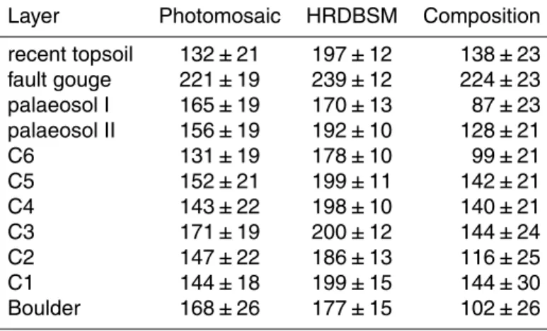
per pixel. Luminance at 1500 nm detected by t-LiDAR significantly differs in some parts

of the trench wall (Fig. 4b and c). As shown in Table 1, the light fault gouge material is highly reflective in both photomosaic and HRDBSM.

The homogeneous silty layer contains only a view voids due to excavation works that influence reflectance value range. Resultant colorimetric shift expressed by the

(15)

SED

7, 2697–2733, 2015

stratigraphy

Title Page

Tables Figures

◭ ◮

Back Close

Full Screen / Esc

Discussion

P

a

per

|

Discussion

P

a

per

|

Discussion

P

a

per

|

Discussion

P

a

per

|

component composition almost solely depicts the highest value ranges for this part of the trench wall (Fig. 4d). In contrast, the cemented colluvium to the west is highly irregu-lar in the sense of reflectance. Both photomosaic and HRDBSM show a heterogeneous greyscale value distribution that is even more embodied by high-grade contrasts in the two-channel composition. Similar observations occur for larger boulders that protrude

5

out of the trench wall (Fig. 4a–d).

Colluvial layers C2–C5 are distinctively different in their reflectance characteristics. Where transition between both units is indeed visible in the photomosaic, a sharp contrast in reflectance characteristics of near-infrared is recognisable. Moreover, the

named colluvial deposits do not only appear as a conglomerate of diffuse values but

10

show evidence of alignments. An upward oriented structure of approximately 0.5 m thickness is obvious in HRDBSM and false colour composition. The structure follows a lineament of displacement within the colluvial strata.

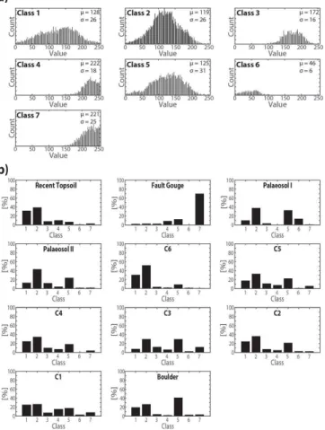
Figure 5 visualises percentages of seven classes, estimated from the unsupervised classification on individual identified layers within the trench log. Either the majority

15

of a certain layer is fulfilled by one single class or by a certain composition of two or three classes. Where Table 1 shows the dominance of high values within the fault gouge layer, the illustration of unsupervised classification proves this layer to be almost completely (70 %) represented by one single class (7). Although class 4 covers almost the same value range as class 7, fault gouge exposure is only covered by 8 % by class

20

4 (see Fig. 5a).

In the unsupervised classification, the fault gouge is the only layer in this trench wall where the majority is covered by one single class. Palaeosol I and palaeosol II have a similar ratio of effecting classes but class 6 is not present in the palaeosol II signature, allowing them to be differentiated. By visualising the spatial arrangement of

25

(16)

SED

7, 2697–2733, 2015

stratigraphy

Title Page

Tables Figures

◭ ◮

Back Close

Full Screen / Esc

Discussion

P

a

per

|

Discussion

P

a

per

|

Discussion

P

a

per

|

Discussion

P

a

per

|

especially in the lower part of palaeosol I is obviously different from any other cluster in palaeosol II, although quantitative statistics conclude a similar composition of classes. Except for C6, which is well represented to around 80 % by class 1 (31 %) and 2 (52 %), and C1, which appears as a unsorted conglomerate of classified responses, the remaining colluvial lithologies appear with similar ratios, especially classes 1, 2,

5

and 5. In a quantitative way no distinction can be recognised. Also, large scale cluster-ing of classes within the layers is absent. However, arrangements, especially of class 7, are obvious and coincide with coarse-grained gravels within the colluvium. Within C3 a micro-cluster of approximately 25 pixels are arranged along a slightly bent line

dipping about 50◦towards the footwall. A similar arrangement of class 7 with an even

10

smaller cluster (3×3 pixels) and wider spread is indicated in C5 dipping 15◦ towards

the footwall. Furthermore, the surrounding matrix is slightly more expressed by class 5 in C5, whereas C3 has subjectively no preferred matrix content (Fig. 4). Alterations are expected to decrease with increasing depth. Dependent on rock composition and mean annual precipitation, the formation of new minerals is commonly related to depth

15

from surface. C4 does not show any spectroscopical attribute except for a complete ab-sence of class 6 and low range greyscale values (see Fig. 5a). Clasts or large boulders protruding out of the trench wall are represented by intermediate value range class 5 on top and wide value range class 1 at the bottom (Fig. 4c).

4.1.3 GPR

20

Using the trench log and multispectral information enables radar facies to be distin-guished. Figure 6 confirms the distinction of individual layers by comparison of re-flected electromagnetic signal intensity. Reflections of visible and near-infrared light within certain zones that fit with trace increment and dimensions of the GPR system (30 cm×2 cm) were sampled and correlated with the radar’s first arrival. As the vertical

25

resolution is a quarter of the wavelengthλ (here: 30–40 cm), we averaged reflection

(17)

SED

7, 2697–2733, 2015

stratigraphy

Title Page

Tables Figures

◭ ◮

Back Close

Full Screen / Esc

Discussion

P

a

per

|

Discussion

P

a

per

|

Discussion

P

a

per

|

Discussion

P

a

per

|

A good correlation between backscattered signals of both passive and active meth-ods is obvious in some parts. A significant contrast in all three datasets is traced by the abrupt transition from fault gouge to palaeosol I (see Figs. 4c and 6). Where reflections of visible and near-infrared light are intense on the surface of the fault gouge expo-sure, they rapidly decrease in signal strength on the palaeosol surface. The opposite

5

reflectance behaviour is observed for radar reflections in the very shallow subsurface; the first lithological transition is characterised by the change of low to moderate re-flection amplitudes in the fine-grained homogeneous fault gouge to higher rere-flection intensities from heterogeneous palaeosol I.

Moderate reflectance with intermediate variance designates the exposure of

10

palaeosol I. A slightly decreasing trend is obvious within this section just before an abrupt rise in both visible and near-infrared light reflection values. This changeover is not obvious from GPR mean values. However, value range given by standard deviation reach wider than the in previous section. Moreover, there is little distinction between individual colluvial deposits from GPR reflection amplitudes.

15

As previously stated, the HRDBSM shows an unrecognised feature in the middle of the trench exposure. A change is proven by a drastic drop in reflections from the GPR signal approximately 3 m from the fault plane. At the same position there is also a minor photomosaic and HRDBSM value decline. Thus, a conspicuous progression similar to a Gaussian bell shape curve in the middle of a dataset is obvious.

20

Layer C1 is not individually considered since the coupling of the antenna on heavily

weathered cemented material with rugged surface relief was not sufficient. However,

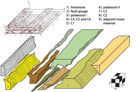
other transitions recognised in trench log and imaging spectroscopy can be traced in GPR images. This then leads to a 3-D model of coseismic features within the hanging-wall (Fig. 7). Seven out of the ten (boulders are not included as an individual layer)

25

previously mapped units plus the limestone fault plane to the West and the adjacent loose material to the East can be traced at depth using GPR.

(18)

SED

7, 2697–2733, 2015

stratigraphy

Title Page

Tables Figures

◭ ◮

Back Close

Full Screen / Esc

Discussion

P

a

per

|

Discussion

P

a

per

|

Discussion

P

a

per

|

Discussion

P

a

per

|

gouge clearly differ in GPR images. Also, the cemented colluvium C1 is characterised

by continuous and high amplitude reflections. Coarse grained components within other colluvial layers are represented as signal scattering hyperbolae within a homogeneous matrix facies. However, a distinction between C4, C5 and, C6 could not be done with

these data. The two palaeosols differ in the recorded intensity of the reflected

elec-5

tromagnetic waves. Where palaeosol I is characterised by high amplitude reflections, palaeosol II contains only minor reflection hyperbolae caused by small clasts within the homogeneous matrix.

4.2 The Kaparelli Fault, Gulf of Corinth

The description of the Kaparelli fault trench follows the lithological designations of

10

Kokkalas et al. (2007). The hanging-wall and footwall of the Kaparelli fault are clearly

separated by a 70–80◦south dipping fault zone. This zone is characterised by a chaotic

assemblage of sheared deposits and material from surrounding or overlying units that has fallen into cracks and fissures. The footwall consists of multi-coloured pebbly-cobbly gravel deposits with a wide range of coarse-grained sub-angular to well-rounded

15

clasts in a silty cemented matrix. The hanging-wall block comprises thick deposits of sandy silt (loess deposits) with many steeply dipping fissure fills, some cutting the en-tire trench wall and others only partly. The fissure thicknesses ranges from around 10 cm to over 80 cm and are filled with sub-angular to rounded gravel deposits in a silty matrix (Fig. 8a).

20

The manually sketched trench log, calibrated using the results from Kokkalas et al. (2007), correlates well with the results from imaging spectroscopy (Fig. 8a). Coarse grained parts of the exposure to the northern end exhibit a widespread range of greyscale values in both photomosaic and HRDBSM. Due to a grain size in the or-der of tens of centimetres and the resulting rough relief, shadows are generated in

25

(19)

SED

7, 2697–2733, 2015

stratigraphy

Title Page

Tables Figures

◭ ◮

Back Close

Full Screen / Esc

Discussion

P

a

per

|

Discussion

P

a

per

|

Discussion

P

a

per

|

Discussion

P

a

per

|

2007), is obvious. Few and much smaller clasts in this unit (diameter is about 1 cm,

<15 %) and a homogeneous matrix have led to a uniform display in the false colour

image. This composition of concurrent greyscale values in the photomosaic and the

HRDBSM occurs three times in constant offsets along the trench exposure. Pure silt

underlies the silty sand. A fissure fill structure of pebbly gravel, dipping about 70◦ to

5

the south, separates the two blocks of silty-sand and silt layers. Again, a rougher re-lief leads to a large range of backscattered signal values from both active and passive systems. However, sharp delimitations of juxtaposed lithological units based on their spectroscopic appearance are clear and discernible. A buried soil horizon and a collu-vial wedge resulting from the 1981 surface rupturing event (Kokkalas et al., 2007) are

10

visible and clearly textured by a certain composition of greyscale values.

In Fig. 8b, a three-dimensional reconstruction of the trench wall shows that exposed structures do not only occur on the surface but are also traceable into the hanging-wall.

Using layer di_fferentiation from imaging spectroscopy helps to recognise certain radar

facies even when there are only subtle distinctions. Major components of the trench

15

wall are identified in individual GPR images. Their three-dimensional extension infor-mation is assembled by interpolating between multiple overlaying GPR images. Hence, information on continuation into depth as well as the varying thicknesses of individual layers is gathered. For instance, the colluvial wedge has only a minor variation in its thickness to 2 m penetration. The estimated average for this unit is 0.6 m.

20

5 Discussion

Trenching investigations have been one of the established methods in palaeoseismic research for the last decades. However, the outcome is highly dependent on the ability of the trench logger to define mappable units and the influence of sunlight. Further-more, producing an accurate log and interpretation requires experience and excellent

25

(20)

SED

7, 2697–2733, 2015

stratigraphy

Title Page

Tables Figures

◭ ◮

Back Close

Full Screen / Esc

Discussion

P

a

per

|

Discussion

P

a

per

|

Discussion

P

a

per

|

Discussion

P

a

per

|

a multispectral view of the palaeoseismic exposure, which allows quantitative informa-tion to be assigned to mapped units within the trench wall.

There are some significant disadvantages of passive data collection imaging

tech-niques. These are mainly due to differing angles of illumination because the trench

ex-posure is not a perfectly even surface at all scales; at larger scales surface undulations

5

dramatically increase. Thus, the lightest parts in the photomosaic, visualised for the Sfaka roadcut as class 7 with an average value of 221, mainly represent a high matrix luminance and the top (bright) sides of boulders and clasts. Rectification and paral-lax effects yield an additional error in the order of a few centimetres. High-resolution 3-D images and the near infrared backscatter signal from t-LiDAR provide

informa-10

tion on the physical properties of materials. Colour, matrix specifications, geometrical alignments and soil formation features influence the t-LiDAR backscatter signal. A mul-tispectral approach, using unsupervised clustering on both spectra supports the results from the trench log and complements the findings. Thereby, a distinct layer signature given by particular compositions of effecting classes allows adjacent stratigraphic units

15

to be differentiated. Some areas within the multispectral image lack evidence for

dis-tinct spectroscopical characteristics. However, these areas can still be defined when they are adjacent to areas with static characteristics; the boundary between two areas is clearly defined as long as one area can be classified using the unsupervised cluster-ing. Therefore, a spectroscopically inconspicuous and completely heterogeneous area

20

surrounded by regions with static characteristics is still sufficiently confined. Within a given error range due to manual gridding on the trench wall, georectification and blending pixels of the photomosaic data, the results show many resemblances to the manually drawn trench log.

The results of the imaging spectroscopy verified the lithology of the trench wall and

25

the resulting image from the unsupervised classification serves as a calibration factor for GPR measurements. Due to the GPR’s resolution being about 0.1 m, the calibration

is necessary to recognise and interpret minor differences in sedimentological

(21)

SED

7, 2697–2733, 2015

stratigraphy

Title Page

Tables Figures

◭ ◮

Back Close

Full Screen / Esc

Discussion

P

a

per

|

Discussion

P

a

per

|

Discussion

P

a

per

|

Discussion

P

a

per

|

be made, which are needed to correlate the amount of vertical offset caused by a

spe-cific surface rupturing event (e.g. Reiss et al., 2003). The quality of the 3-D GPR image and its interpretation depends on well-structured data acquisition and processing, as well as on the experience of the operator. The coupling of the antenna to the surface is decreased on bumpy surfaces, which leads to lower quality data. Moreover, the

ref-5

erence grid on the surface poses a source for stumbling. However, the grid is needed to fuse the geophysical data with remotely collected data and to locate the GPR im-ages in three-dimensional space. An alternative to a grid made of string is colour spray to mark locations for orientation; but, these would have a significant impact on the re-sults from imaging spectroscopy. When the survey is accurately planned and organised

10

good results can be obtained which allow a 3-D interpretation of sedimentary features to between 2 and 3 m depth within the trench wall.

The biggest disadvantage of the presented workflow is by far the effect of sediment

moisture content on reflectance, both in the multispectral analysis and GPR survey. For the multispectral analysis there is not only darkening of the sediments, which leads

15

to an overall reduction of reflectance, but significant partial absorptions at wavelengths near 1.4 and 1.9 µm is also common (Lobell and Asner, 2002; Ragona et al., 2006).

Moreover, water content in a given medium leads to distortion effects and high

atten-uations of electromagnetic waves (Neal, 2004; Schrott and Sass, 2008). However, for conditions when the moisture content is similar throughout the trench wall, water

ab-20

sorptions should not affect the correlations because reflectance along the wall should

be affected uniformly. Ragona et al. (2006) have shown that identifying stratigraphy

with samples that maintain high amounts of their original moisture content is possible; however, we reiterate the authors’ suggestion to consider necessary approaches to minimise changing reflectance.

25

Other potential error sources using this technique are dependent on the character-istics of the individual trenching sites and the equipment used. Some sites are hard to access because of steepness, height and/or width of the excavation. Extremely steep

(22)

SED

7, 2697–2733, 2015

stratigraphy

Title Page

Tables Figures

◭ ◮

Back Close

Full Screen / Esc

Discussion

P

a

per

|

Discussion

P

a

per

|

Discussion

P

a

per

|

Discussion

P

a

per

|

heights exceeding usual body heights generate problems for the GPR survey; these

can be overcome using ropes and wooden tools to ensure good coupling. Scaff

old-ing usually consists of metal which may lead to interferences in the GPR image. If the trench wall is not properly prepared in terms of cleaning, or the embedded sed-iments produce a rough surface because of coarser grain sizes, spectral amplitudes

5

will change because of varying illumination and incident angles. Therefore, the

spectro-scopic interpretation must take these accompanying effects into account. Moreover,

ex-tremely complex sedimentological architectures may cause complicated multi-pathing

effects on the radar waves. The presented workflow has basic requirements

concern-ing computconcern-ing capacities; the collected high-resolution data from conventional photo

10

cameras, t-LiDAR scanning and GPR measurements engage substantial disk space and random access memory.

One major benefit from this workflow is the storage and future use of the raw data. The majority of paleoseismic trenches are designed to be closed after field investiga-tions are completed. This means that not only is there no future access to these

ex-15

posures, but the sedimentological environment of the excavated site is also destroyed. If a trench is left open after field investigations, the trench walls will get degraded and

altered by weathering effects. t-LiDAR and GPR measurements provide and store

infor-mation on the visual appearance of the trench and the reflection properties of different electromagnetic wavebands. The reflectance spectrum at each pixel of an image

pro-20

vides unbiased compositional information. This saved data can always be used for future (re-)analyses.

6 Conclusions

Identifying and mapping individual lithological units along a palaeoseismological expo-sure in accordance with colour and matrix specifications as well as sedimentary

struc-25

(23)

SED

7, 2697–2733, 2015

stratigraphy

Title Page

Tables Figures

◭ ◮

Back Close

Full Screen / Esc

Discussion

P

a

per

|

Discussion

P

a

per

|

Discussion

P

a

per

|

Discussion

P

a

per

|

the experience of the trench logger, and is thus subjectively influenced. Hence, (minor)

differences in lithological description from expert to expert are expected, especially

if one logger has access to no more than a photomosaic. In order to prove whether conventional trench logging methods used to map coseismic features in a palaeoseis-mic trench wall can be objectively enhanced, we created an accurate digital version of

5

the exposure and its physical properties. This was done by combining routine logging with vertical GPR measurements and imaging spectroscopic approaches from nor-malised photomosaics and high resolution t-LiDAR backscatter models. Both the stud-ied palaeoseimsic exposures, on Crete and in mainland Greece, exhibit sedimentary structures whose constituent parts and shape are essential information for a

palaeo-10

seismic reconstruction.

After the conventional trench logging was completed, t-LIDAR scans were under-taken at close range. The near-infrared backscattered signal was combined with a lu-minance bearing photomosaic of the same trench wall. Statistical and classification techniques reproduce an objective digital copy of a palaeoseismic trench log. In order

15

to define distinct units, four options to characterise and differentiate individual layers by imaging spectroscopy can be registered:

– Significant dominance of a certain class within a distinct layer.

– Certain composition with spatial clustering.

– Certain composition with certain arrangements.

20

– Distinct borders between individual layers although one or both are not

deter-mined by applied statistics.

Subtle or invisible features are enhanced and become part of a quantitative analy-sis, and comparisons of units using their reflectance on certain wavelengths (see also Ragona et al., 2006) can be carried out. Our results show that based on distinct layers

25

(24)

SED

7, 2697–2733, 2015

stratigraphy

Title Page

Tables Figures

◭ ◮

Back Close

Full Screen / Esc

Discussion

P

a

per

|

Discussion

P

a

per

|

Discussion

P

a

per

|

Discussion

P

a

per

|

the spatial extent of palaeoseismic features can be traced within the trench wall. The resulting 3-D model from the GPR provides information on representative layer thick-nesses, displacements, and geometries. This is highly beneficial since it minimises misinterpretation due to cutting effects.

Reconstructing the paleoseismological history of both trench exposures is not an

in-5

tegral part of this paper, but this research has shown that recognising individual event layers can be improved using multispectral viewing and 3-D visualisation of GPR im-ages. This method can therefore contribute to the accuracy of seismic hazard assess-ment.

Acknowledgements. We thank Aggelos Pallikarakis from the Agricultural University of Athens

10

for his cooperation and assistance on Crete and in Mainland Greece. Silke Mechernich, Lauretta Kärger, Tobias Baumeister, and Alexander Woywode supported our fieldwork. In Pachia Ammos, the Zorbas Taverna is thanked for the loan of equipment and excellent food.

The authors would like to thank Christoph Grützner from Cambridge University for his valu-able comments regarding the manuscript.

15

References

Alasset, P.-J. and Meghraoui, M.: Active faulting in the western Pyrénées (France): paleoseis-mic evidence for late Holocene ruptures, Tectonophysics, 409, 39–54, 2005.

Ambraseys, N. N. and Jackson, J. A.: Seismicity and associated strain of central Greece be-tween 1890 and 1988, Geophys. J. Int., 101, 663–708, 1990.

20

Benedetti, L., Finkel, R., Papanastassiou, D., King, G., Armijo, R., Ryerson, F., Farber, D., and Flerit, F.: Post-glacial slip history of the Sparta fault (Greece) determined by 36 Cl cosmogenic dating: evidence for non-periodic earthquakes, Geophys. Res. Lett., 29, doi:10.1029/2001GL014510, 2002.

Benedetti, L., Finkel, R., King, G., Armijo, R., Papanastassiou, D., Ryerson, F. J., Flerit, F.,

25

(25)

SED

7, 2697–2733, 2015

stratigraphy

Title Page

Tables Figures

◭ ◮

Back Close

Full Screen / Esc

Discussion

P

a

per

|

Discussion

P

a

per

|

Discussion

P

a

per

|

Discussion

P

a

per

|

Bubeck, A., Wilkinson, M., Roberts, G. P., Cowie, P. A., McCaffrey, K., Phillips, R., and Sam-monds, P.: The tectonic geomorphology of bedrock scarps on active normal faults in the Italian Apennines mapped using combined ground penetrating radar and terrestrial laser scanning, Geomorphology, 237, 38–51, 2015.

Bull, W. B.: Tectonic Geomorphology of Mountains: a New Approach to Paleoseismology,

Black-5

well Pub., Malden, MA, 316 pp., 2007.

Carcaillet, J., Manighetti, I., Chauvel, C., Schlagenhauf, A., and Nicole, J.-M.: Identifying past earthquakes on an active normal fault (Magnola, Italy) from the chemical analysis of its exhumed carbonate fault plane, Earth Planet. Sc. Lett., 271, 145–158, 2008.

Chow, J., Angelier, J., Hua, J.-J., Lee, J.-C., and Sun, R.: Paleoseismic event and active

fault-10

ing: from ground penetrating radar and high-resolution seismic reflection profiles across the Chihshang Fault, eastern Taiwan, Tectonophysics, 333, 241–259, 2001.

Demanet, D., Renardy, F., Vanneste, K., Jongmans, D., Camelbeeck, T., and Meghraoui, M.: The use of geophysical prospecting for imaging active faults in the Roer Graben, Belgium, Geophysics, 66, 78–89, 2001.

15

De Rose, R. C., Oguchi, T., Morishima, W., and Collado, M.: Land cover change on Mt. Pinatubo, the Philippines, monitored using ASTER VNIR, Int. J. Remote Sens., 32, 9279– 9305, 2011.

Gaki-Papanastassiou, K., Karymbalis, E., Papanastassiou, D., and Maroukian, H.: Quaternary marine terraces as indicators of neotectonic activity of the Ierapetra normal fault SE Crete

20

(Greece), Geomorphology, 104, 38–46, 2009.

Grützner, C., Reicherter, K., Hübscher, C., and Silva, P. G.: Active faulting and neotectonics in the Baelo Claudia area, Campo de Gibraltar (southern Spain), Tectonophysics, 554–557, 127–142, 2012.

Grützner, C., Barba, S., Papanikolaou, I. D., and Pérez-López, R.: Earthquake geology: science,

25

society and critical facilities, Ann. Geophys.-Italy, 56, S0683, doi:10.4401/ag-6503, 2013. Höfle, B. and Pfeifer, N.: Correction of laser scanning intensity data: data and model-driven

approaches, ISPRS J. Photogramm., 62, 415–433, 2007.

Jackson, J. A., Gagnepain, J., Houseman, G., King, G., Papadimitriou, P., Soufleris, C., and Virieux, J.: Seismicity, normal faulting, and the geomorphological development of the Gulf of

30

(26)

SED

7, 2697–2733, 2015

stratigraphy

Title Page

Tables Figures

◭ ◮

Back Close

Full Screen / Esc

Discussion

P

a

per

|

Discussion

P

a

per

|

Discussion

P

a

per

|

Discussion

P

a

per

|

Jörg, P., Fromm, R., Sailer, R., and Schaffhauser, A.: Measuring snow depth with a terrestrial laser ranging system, International Snow Science Workshop, 1–6 October 2006, Telluride, CO, USA, 452–460, 2006.

Keller, E. A. and Rockwell, T. K.: Tectonic Geomorphology, Quaternary chronology, and Pale-oseismicity, in: Tectonic Geormophology, Quaternary Chronology, and PalePale-oseismicity,

De-5

velopments and Applications of Geomorphology, edited by: Costa, J. E. and Fleisher, P. J., Springer, Berlin, Heidelberg, 203–239, 1984.

Kokkalas, S. and Koukouvelas, I. K.: Fault-scarp degradation modeling in central Greece: the Kaparelli and Eliki faults (Gulf of Corinth) as a case study, J. Geodyn., 40, 200–215, 2005. Kokkalas, S., Pavlides, S., Koukouvelas, I. K., Ganas, A., and Stamatopoulos, L.: Paleoseimicity

10

of the Kaparelli fault (eastern Corinth Gulf): evidence for earthquake recurrence and fault behaviour, Boll. Soc. Geol. Ital., 126, 387–395, 2007.

Le Pichon, X. and Angelier, J.: The hellenic arc and trench system: a key to the neotectonic evolution of the eastern mediterranean area, Tectonophysics, 60, 1–42, 1979.

Lobell, D. B. and Asner, G. P.: Moisture effects on soil reflectance, Soil Sci. Soc. Am. J., 66,

15

722–727, doi:10.2136/sssaj2002.7220, 2002.

Lyon-Caen, H., Armijo, R., Drakopoulos, J., Baskoutass, J., Delibassis, N., Gaulon, R., Kousk-ouna, V., Latoussakis, J., Makropoulos, K., Papadimitriou, P., Papanastassiou, D., and Pe-dotti, G.: The 1986 Kalamata (South Peloponnesus) Earthquake: detailed study of a normal fault, evidences for east–west extension in the Hellenic Arc, J. Geophys. Res., 93, 14967,

20

doi:10.1029/JB093iB12p14967, 1988.

Machette, M. N.: Active, capable, and potentially active faults – a paleoseismic perspective, J. Geodyn., 29, 387–392, 2000.

Mariolakos, I. and Papanikolaou, D. J.: The Neogene basins of the Aegean Arc from the Pa-leogeographic and the Geodynamic point of view, in: Proc. Int. Symp. H. E. A. T., Athens,

25

Greece, 8–10 April 1981, 383–399, 1981.

McCalpin, J.: Paleoseismology, 2nd edn., International Geophysics Series, v. 95, Academic Press, Burlington, MA, 613 pp., 2009.

McKenzie, D.: Active tectonics of the Mediterranean region, Geophys. J. Roy. Astr. S., 30, 109– 185, 1972.

30