www.biogeosciences.net/8/2665/2011/ doi:10.5194/bg-8-2665-2011
© Author(s) 2011. CC Attribution 3.0 License.
Biogeosciences
Quantification of terrestrial ecosystem carbon dynamics in the
conterminous United States combining a process-based
biogeochemical model and MODIS and AmeriFlux data
M. Chen1, Q. Zhuang1,2, D. R. Cook3, R. Coulter3, M. Pekour4, R. L. Scott5, J. W. Munger6, and K. Bible7
1Department of Earth & Atmospheric Sciences, Purdue University, West Lafayette, IN, USA 2Department of Agronomy, Purdue University, West Lafayette, IN, USA
3Climate Research Section, Environmental Science Division, Argonne National Laboratory, Argonne, IL, USA 4Atmospheric Sciences and Global Change Division, Pacific Northwest National Laboratory, Richland, WA, USA 5Southwest Watershed Research Center, USDA-ARS, Tucson, AZ, USA
6Division of Engineering and Applied Sciences and Department of Earth and Planetary Sciences, Harvard University, Cambridge, MA, USA
7Wind River Canopy Crane Research Facility, University of Washington, WA, USA Received: 15 February 2011 – Published in Biogeosciences Discuss.: 16 March 2011 Revised: 22 August 2011 – Accepted: 9 September 2011 – Published: 21 September 2011
Abstract. Satellite remote sensing provides continuous
temporal and spatial information of terrestrial ecosystems. Using these remote sensing data and eddy flux measure-ments and biogeochemical models, such as the Terrestrial Ecosystem Model (TEM), should provide a more adequate quantification of carbon dynamics of terrestrial ecosystems. Here we use Moderate Resolution Imaging Spectroradiome-ter (MODIS) Enhanced Vegetation Index (EVI), Land Sur-face Water Index (LSWI) and carbon flux data of AmeriFlux to conduct such a study. We first modify the gross primary production (GPP) modeling in TEM by incorporating EVI and LSWI to account for the effects of the changes of canopy photosynthetic capacity, phenology and water stress. Sec-ond, we parameterize and verify the new version of TEM with eddy flux data. We then apply the model to the con-terminous United States over the period 2000–2005 at a 0.05◦×0.05◦ spatial resolution. We find that the new
ver-sion of TEM made improvement over the previous verver-sion and generally captured the expected temporal and spatial patterns of regional carbon dynamics. We estimate that re-gional GPP is between 7.02 and 7.78 Pg C yr−1and net pri-mary production (NPP) ranges from 3.81 to 4.38 Pg C yr−1 and net ecosystem production (NEP) varies within 0.08– 0.73 Pg C yr−1over the period 2000–2005 for the contermi-nous United States. The uncertainty due to parameterization
Correspondence to:M. Chen ([email protected])
is 0.34, 0.65 and 0.18 Pg C yr−1for the regional estimates of GPP, NPP and NEP, respectively. The effects of extreme cli-mate and disturbances such as severe drought in 2002 and destructive Hurricane Katrina in 2005 were captured by the model. Our study provides a new independent and more ade-quate measure of carbon fluxes for the conterminous United States, which will benefit studies of carbon-climate feedback and facilitate policy-making of carbon management and cli-mate.
1 Introduction
is between 0.30 and 0.58 Pg C yr−1(1 Pg = 1015g) over the 1980s. Fan et al. (1998) estimated the North America sink as 1.7±0.5 Pg C yr−1over the period of 1988 to 1992, mostly in the south of 51◦N. Analyses based on land use change and inventory databases for the conterminous United States in the 1980s estimated a sink of 0.08 to 0.35 Pg C yr−1 (Turner et al., 1995; Houghton et al., 1999, 2000; Houghton and Hack-ler, 2000). Results from the Vegetation/Ecosystem Model-ing and Analysis Project (VEMAP) suggested a smaller sink (0.08±0.02 Pg C yr−1)of the conterminous United States from 1980 to 1993 (Schimel et al., 2000). Recently, Potter et al. (2007) estimated a sink of 0.04 to 0.2 Pg C yr−1from 2000 to 2004 while Xiao et al. (2008) estimated the sink at 0.68 Pg C yr−1 over the period 2000 to 2006 using satellite information. Overall, these results have shown great uncer-tainties, and remarkably, the uncertainty sometimes is larger than the sink itself.
Reducing the uncertainty of large-scale carbon exchanges requires more adequate comprehension to the related bio-physical processes. Traditionally, process-based biogeo-chemical models have been used (e.g. Raich et al., 1991; Potter et al., 1993; Field et al., 1995; Zhuang et al., 2003; Running and Hunt Jr., 1993). These models usually consider carbon fluxes as functions of climatic and biogeochemical factors (McGuire et al., 1992) and are able to estimate car-bon fluxes and storage in the ecosystem. However, since the environmental limitation for simulating carbon fluxes is esti-mated with specific algorithms driven by uncertain environ-mental variables, biases between the observed and estimated environmental status can introduce uncertainty. In addition, terrestrial biogeochemical model simulations are uncertain due to lacking of large-scale disturbance data (Canadell et al., 2000; Law et al., 2006). Remotely sensed data provide glob-ally consistent and near real-time observations of numerous surface variables as well as the information of the timing, dis-tribution, spatial extent or severity of disturbances at regional and global scales (Zhao and Running, 2008). These satellite data help more adequately quantify carbon dynamics (Coops et al., 1998; Seaquist et al., 2003; Xiao et al., 2004; Sims et al., 2008). These remotely-sensed data are good at esti-mating carbon assimilation and plant respiration, but not het-erotrophic respiration. Satellite-based models alone cannot sufficiently account for vegetation carbon (Xiao et al., 2010) and nitrogen availability (Clark et al., 1999, 2004) while these can be provided by process-based models. Therefore, models that are based on both satellite observations and bio-geochemical processes could potentially improve the quan-tification of carbon dynamics of Gross Primary Production (GPP), Autotrophic Respiration (RA)and heterotrophic res-piration (RH). For example, Potter et al. (2003) retrieved ma-jor disturbances at a global scale with the AVHRR FPAR data for the period of 1982–1999 and combined them with the NASA-CASA model to estimate the above-ground biomass carbon lost. Hazarika et al. (2005) used MODIS derived Leaf Area Index (LAI) to constrain an ecosystem model
(Sim-CYCLE) and improved the accuracy in estimating global Net Primary Production (NPP). However, limitations still exist in those studies. For example, the NASA-CASA directly mod-eled NPP but avoided the estimation of the Gross Primary Production (GPP). The MODIS LAI products used for con-straining Sim-CYCLE are not directly calculated with sur-face reflectance but derived with complex algorithms (My-neni et al., 2002) which can cause high uncertainty. Here we conduct a study by combining satellite reflectance data with a process-based biogeochemistry model, the Terrestrial Ecosystem Model (McGuire et al., 1992, 2001; Zhuang et al., 2003; Raich et al., 1991), to quantify the carbon dynamics in the conterminous US for the period of 2000–2005.
Eddy covariance flux towers have been established since the 1990s to provide continuous measurements of ecosystem-level carbon exchanges (Wofsy et al., 1993; Bal-docchi et al., 2001). At present, over 400 eddy covariance flux towers are operating on a long-term and continuous basis over the globe (FLUXNET http://daac.ornl.gov/FLUXNET/ fluxnet.shtml). This global network covers a wide range of climate and biome types, and provides probably the best measurements of Net Ecosystem carbon Exchange (NEE) (Xiao et al., 2008). Previous ecosystem models were either estimated or calibrated with annual values of observed car-bon fluxes (Raich et al., 1991; Potter et al., 1993) and the time series data of carbon fluxes have not been adequately used. In recent years, a number of studies used eddy flux data in a model-data fusion manner to improve the parameteriza-tion and predictability of process-based ecosystem models (e.g. Tang and Zhuang, 2008, 2009; Braswell et al., 2005; Williams et al., 2005; Aalto et al., 2004; Santaren et al., 2007; Wang et al., 2001, 2007). Here we conduct a model-data fusion study with a satellite-based model. We first develop a new version of TEM based on satellite-observed surface reflectance, which is hereafter referred to as SAT-TEM. Sec-ond we parameterize the SAT-TEM using flux tower data and compare both SAT-TEM and TEM performance at the site level. Finally, we use SAT-TEM to quantify carbon fluxes in the conterminous United States in comparison with the esti-mates of a previous version of TEM.
2 Method
2.1 Overview
by incorporating MODIS EVI and LSWI. We then use a Bayesian Inference technique (Tang and Zhuang, 2009) to parameterize the model. The model is then verified for dif-ferent ecosystem types with the observed Net Ecosystem Ex-change (NEE) and GPP from eddy covariance flux towers of AmeriFlux network. To examine how the new model could improve the carbon flux estimation of TEM, we run both ver-sions of TEM at the same sites with the same driving data sets. The model is finally applied to estimate dynamics of carbon fluxes for each 0.05◦×0.05◦grid cell across the
con-terminous United States over the period 2000–2005.
2.2 Modification to the terrestrial ecosystem model
The TEM is a well-documented process-based ecosystem model that describes carbon and nitrogen dynamics of plants and soils for terrestrial ecosystems (Raich et al., 1991; McGuire et al., 1992, 2001; Melillo et al., 1993; Zhuang et al., 2001, 2002, 2003, 2004). The TEM runs at monthly time step and uses spatially referenced information on climate, el-evation, soils, vegetation and water availability as well as soil- and vegetation-specific parameters to make monthly es-timates of important carbon and nitrogen fluxes and pool sizes of terrestrial ecosystems. In TEM, GPP is modeled as a function of irradiance of photosynthetically active radiation (PAR), atmospheric CO2concentrations, moisture availabil-ity, mean air temperature, the relative photosynthetic capac-ity of the vegetation, and nitrogen availabilcapac-ity. The freezing and thawing dynamics have also been considered (Zhuang et al., 2003). The formula for calculating monthly GPP is: GPP=Cmaxf (PAR)f (PHENOLOGY)f (FOLIAGE)
f (T )f (CA,Gv)f (NA)f (FT) (1)
whereCmax is the maximum rate of C assimilation by the entire plant canopy under optimal environmental conditions; f(PAR) represents the influence of photosynthetically ac-tive radiation; f(PHENOLOGY) is monthly leaf area rela-tive to leaf area during the month of maximum leaf area depending on monthly estimated evapotranspiration (Raich et al., 1991); f(FOLIAGE) is a scalar function represent-ing the ratio of canopy leaf biomass relative to maximum leaf biomass (Zhuang et al., 2002) having the similar ef-fect asf(PHENOLOGY) on constraining the estimation of GPP;f (T )is temperature scalar with reference to the deriva-tion of optimal temperatures for plant producderiva-tion andT is monthly air temperature;f (CA,Gv)represents the effect of
CO2 concentrations, whereCA is CO2concentration in the atmosphere andGvis a unitless multiplier that accounts for
changes in leaf conductivity to CO2resulting from changes in moisture availability. The functionf(NA) models the lim-iting effects of plant nitrogen availability. f(FT) is an in-dex of sub-monthly thaw to indicate effects of freeze-thaw dynamics on GPP (Zhuang et al., 2003). In TEM, NPP is defined as the difference of GPP and autotrophic respira-tion (RA)and the net carbon exchange between the
ecosys-tems and atmosphere is defined as NEP, a difference between NPP and heterotrophic respiration (RH)(Raich et al., 1991; McGuire et al., 1992, 2001; Zhuang et al., 2003).
Satellite vegetation indices are widely used in satellite-based carbon models to represent the fraction of vegetation absorbed PAR (FAPAR) (Prince and Goward, 1995; Run-ning et al., 1999, 2000; Potter et al., 1993; Xiao et al., 2004). For example, the Normalized Difference Vegetation Indices (NDVI), which captures the contrast between the visible-red and near-infrared reflectance of vegetation, has a good linear or non-linear relationship of FAPAR. Recent studies show that EVI (Huete et al., 1997, 2002) calculated from the MODIS could more efficiently dismiss the influence of atmospheric scattering and sensitive to canopy variations (Huete et al., 2002). EVI is believed to be a better choice than NDVI to represent photosynthetic activity of vegetation canopy (Boles et al., 2004; Xiao et al., 2004; Yang et al., 2007) and provides reasonably accurate direct estimates of GPP (Rahman et al., 2005). EVI is a normalized index us-ing the reflectance in the near infrared (NIR), red and blue spectral bands:
EVI= 2.5(ρnir−ρred)
ρnir+(6ρred−7.5ρblue)+1
(2) Apart from EVI, Xiao et al. (2004) developed the Vegeta-tion Photosynthesis Model (VPM) which used the Land Sur-face Water Index (LSWI) to help capture the effects of water stress and leaf phenology. As the shortwave infrared (SWIR) spectral band is sensitive to land surface water content, the LSWI is calculated as the normalized difference between NIR and SWIR spectral bands:
LSWI=ρnir−ρswir
ρnir+ρswir (3)
where the SWIR spectral bands may be either 1628–1652 nm or 2105–2155 nm for MODIS on board the NASA Terra satellite (Yan et al., 2009; Ratana et al., 2005; Li et al., 2007). In our study, we use the band at 2105–2155 nm to calculate LSWI.
We therefore adopt the formulae of the VPM for GPP modeling in our revision of TEM. We use water scalar (Wscalar), phenology scalar (Pscalar)and EVI to account for the vegetation water stress and phenology as well as absop-tion of PAR while maintaining the original formulaabsop-tion for nitrogen availability, temperature constraints, and the effect of CO2concentration. GPP in the new version of TEM (SAT-TEM) is thus modeled as:
GPP=Cmaxf (PAR)f (T )WscalarPscalarf (CA,Gv)
f (NA)f (FT) (4)
where f(PAR)=EVI×PAR/(ki+ PAR) indicates the PAR
absorption and the effect of PAR saturation whileki is the
923
924
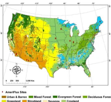
Fig. 1. Land cover map of the conterminous US (0.05◦×0.05◦) used in regional simulations. The map was re-classified based on MODIS product Land Cover Types Yearly L3 Global 0.05 Deg CMG (MOD12C1). Red pins indicate the location of the Ameri-Flux sites used in this study.
we calculated LSWImax in advance and use it as an in-put parameter for each grid cell in the regional simulation. Pscalar=(1 + LSWI)/2. Specifically,Pscalar is set to be 1 for evergreen vegetations (Xiao et al., 2004). The calculations of NPP and NEP in SAT-TEM are kept the same as the previous version of TEM.
2.3 Data organization
2.3.1 Site-level data
To drive SAT-TEM model, we first parameterize SAT-TEM using AmeriFlux site observations. We organize the ob-served GPP, NEP and meteorological data (radiation, air tem-perature, and precipitation) from six representative eddy co-variance flux sites for each vegetation type to parameterize and verify SAT-TEM. In order to further test the performance of SAT-TEM, we organize the same data from ten additional available sites covering all the six vegetation types across most of the conterminous United States (Fig. 1). Specif-ically, we gather all available monthly Level 4 GPP and Net Ecosystem Exchange (NEE) products (http://public.ornl. gov/ameriflux/) at these sites (Table 1). The Level 4 prod-uct consists of two types of NEE data, including standard-ized (NEE st) and original (NEE or) NEE. Corresponding GPP st and GPP or are calculated by ecosystem respiration (Re)with NEE st and NEE or, respectively. GPP st, GPP or, NEE st and NEE or are filled using the Marginal Distribu-tion Sampling (MDS) method (Reichstein et al., 2005) and
the Artificial Neural Network (ANN) method (Papale and Valentini, 2003). We use GPP and NEE calculated from NEE data that were gap-filled using the ANN method (Moffat et al., 2007; Xiao et al., 2008). For each site, if the percent-age of the remaining missing values for NEE st is lower than that for NEE or, we select NEE or and GPP or; otherwise, we use NEE st and GPP st. To compare with our TEM sim-ulation, we treat NEE as TEM NEP, but with different signs. We obtain site-level EVI and LSWI by collecting MODIS ASCII subsets (Collection 5) which consist of 7×7 km re-gions centered on the flux tower from the Oak Ridge Na-tional Laboratory’s Distributed Active Archive Center for each AmeriFlux site. This 16-day product has a spatial res-olution of 1×1 km. To better represent the flux tower foot-print (Schmid, 2002; Rahman et al., 2005; Xiao et al., 2008, 2010), mean EVI, NIR and SWIR band values for the central 3×3 km area are extracted within the 7×7 km cutouts. We only use the pixels with good quality which are determined by the corresponding quality assurance (QA) flags included in the product. LSWIs are then calculated by NIR and SWIR band values. Each 16-day EVI and LSWI values are aggre-gated into monthly values to correspond with the time step of SAT-TEM.
2.3.2 Regional spatially-explicit data
To conduct regional simulations, we organize the regional data of vegetation, soils, topography, and climate at a spa-tial resolution 0.05◦×0.05◦. We obtain land-cover
infor-mation derived from MODIS product Land Cover Types Yearly L3 Global 0.05 Deg CMG (MOD12C1) (Year 2004) from NASA Goddard Space Flight Center website (http: //modis-land.gsfc.nasa.gov). We use the classification of the International Geosphere and Biosphere (IGBP) land-cover classification system to classify the land cover map of the conterminous United States into 6 major vegetation types, which are used in our SAT-TEM simulations (Table 2 and Fig. 1). EVI, NIR and SWIR bands data are extracted from MOD13C2 (MODIS Terra Vegetation Indices Monthly L3 Global 0.05Deg CMG V005) for the conterminous United States.
Mean monthly climate data including air temperature, cloudiness fractions and precipitation are extracted from NCEP global datasets at a 0.5◦spatial resolution (Kistler et
al., 2001). Spatial elevation data and soil texture data from previous studies are from Zhuang et al. (2003). All these data are interpolated into a 0.05◦spatial resolution using Inverse
Distance Weighted method to match MODIS data.
2.4 Model parameterization and application
Table 1.Characteristics of AmeriFlux sites used in this study.
Site Name Latitude Longitude Vegetation Type Years References
(◦) (◦)
Howland Forest West Tower (ME, USA)∗ 45.2091 −68.7470 Evergreen Forest 2000–2004 Hollinger et al. (1999, 2004)
Harvard Forest (MA, USA)∗ 42.5378 −72.1715 Deciduous Forest 2000–2006 Urbanski et al. (2007)
Vaira Ranch (CA, USA)∗ 38.4061 −120.9507 Grassland 2002–2007 Xu and Baldocchi (2004)
Sky Oaks New (CA, USA)∗ 33.3844 −116.6403 Shrubland 2004–2006 Lipson et al. (2005)
Tonzi Ranch (CA, USA)∗ 38.4316 −120.9660 Savannas 2002–2007 Ma et al. (2007)
Bondville (IL, USA)∗ 40.0062 −88.2904 Cropland 2001–2006 Hollinger et al. (2005)
Niwot Ridge (CO, USA) 40.0329 −105.5464 Evergreen Forest 2000–2005 Monson et al. (2002)
Wind River Crane site (WA, USA) 45.8205 −121.9519 Evergreen Forest 2000–2002 Falk et al. (2008)
Morgan Monroe State Forest (IN, USA) 39.3232 −86.4131 Deciduous Forest 2001–2006 Schmid et al. (2000)
Willow Creek (WI, USA) 45.8059 −90.0799 Deciduous Forest 2000–2003 Cook et al. (2004)
Kendall Grassland (AZ, USA) 31.7365 −109.9419 Grassland 2005–2007 Scott et al. (2010)
Walnut River (KS, USA) 37.5208 −96.8550 Grassland 2002–2003 Coulter et al. (2006)
Sky Oaks Old (CA, USA) 33.3739 −116.6229 Shrubland 2004–2006 Lipson et al. (2005)
Santa Rita Mesquite Savanna (AZ, USA) 31.8214 −110.8661 Savannas 2004–2006 Scott et al. (2009)
Rosemount G21 Conventional Management 44.7143 −93.0898 Cropland 2004–2006 Griffis et al. (2008)
Corn Soybean Rotation (MN, USA)
Mead Irrigated Rotation (NE, USA) 41.1649 −96.4701 Cropland 2002–2005 Suyker et al. (2005)
∗Sites for parameterization.
Table 2.Reclassification of MODIS land covers to TEM vegetation types.
MODIS Land Cover Types (IGBP) Vegetation Community Type in SAT-TEM
Evergreen needleaf forest Evergreen Forest
Evergreen broadleaf forest Evergreen Forest
Deciduous needleaf forest Deciduous Forest
Deciduous broadleaf forest Deciduous Forest
Mixed forest 50 % Evergreen Forest,
50 % Deciduous Forest
Closed shrubland Shrubland
Open shrubland Shrubland
Woody savannas Savannas
Savannas Savannas
Grassland Grassland
Permanent Wetland Grassland
Cropland Cropland
Cropland and natural Cropland
vegetation mosaic
follows the procedures described in Tang and Zhuang (2009). Firstly, 15 key parameters (Table 3) are selected to conduct the parameterization according to our previous sensitivity study (Tang and Zhuang, 2009) and parameterization expe-riences. To derive the prior parameter sets of SAT-TEM, we first assume that they follow the uniform distributions within previous specified reasonable ranges either based on litera-ture review or our experience. We sample 500 000 sets of
Table 3.Key TEM Parameters.
Parameter Definition Unit Prior Range
ki Half saturation constant for PAR used by plants µl l−1 [100.0, 500.0]
kc Half saturation constant for CO2-C uptake by plants µl l−1 [100.0, 400.0]
RAQ10A0 Leading coefficient of the Q10 model for plant respiration None [1.0, 3.0]
RAQ10A1 1st order coefficient of the Q10 model for plant respiration ◦C−1 [−0.1, 0.1]
RAQ10A2 2nd order coefficient of the Q10 model for plant respiration ◦C−2 [0, 0.005]
RAQ10A3 3rd order coefficient of the Q10 model for plant respiration ◦C−3 [0.0001, 0.001]
RHQ10 Change in heterotrophic respiration rate due to 10◦C temperature increase None [1.0, 3.0]
MOISTOPT Optimum soil moisture content for heterotrophic respiration % [20, 80]
Cmax Maximum rate of photosynthesis C g C m−2month−1 [500.0, 3000.0]
Kr Logarithm of plant respiration rate at 0◦C g g−1month−1 [−9.5,−0.2]
Kd Heterotrophic respiration rate at 0◦C g g−1month−1 [0.0005, 0.007]
KFALL Proportion of vegetation carbon loss as litterfall monthly g g−1month−1 [0.0005, 0.005]
Nmax Maximum rate of N uptake by vegetation g m−2month−1 [0.1, 1.0]
Nup Ratio between N immobilized and C respired by heterotrophs g g−1 [0, 0.05]
NFALL Proportion of vegetation nitrogen loss as litter-fall monthly g g−1month−1 [0.001, 0.01]
The parameterized SAT-TEM is then applied to the conter-minous United States for the period of 1948–2005 at a 0.05◦
spatial resolution with a total of 322 287 grid cells. We first run SAT-TEM to equilibrium with the long-term averaged climate and CO2concentration data from 1948 to 2005. We then spin-up the model for 120 yr to account for the influence of climate inter-annual variability on the initial conditions of the ecosystems. Since historic climate and CO2 concentra-tion data are not available before 1948, we repeat the data from 1948 to 1987 for 3 times for the spin-up. In addition, since MODIS vegetation index products are only available from 2000, we fill the gap by repeating 2000–2005 MODIS EVI data for the whole period in order to have consistent data for our simulation period. After the spin-up, we run the model with transient monthly climate and annual atmo-spheric CO2concentrations from 1948 to 2005 and then ex-tract the results of the period of 2000–2005 for further analy-sis. To quantify the uncertainty of regional simulation caused by parameterization, we run ensemble SAT-TEM simulations with the 50 sets of parameters obtained from site-level pa-rameterizations. The averaged values and standard devia-tions of 50 sets of regional results are calculated for analysis. For comparison, we also conduct a regional simulation with TEM.
3 Results and discussion
3.1 Model performance at AmeriFlux sites
The parameterized SAT-TEM can reproduce the carbon fluxes reasonably well at the six parameterization sites. Com-parisons at each individual site show reasonable agreement of seasonality and inter-annual variability between the
ob-served and predicted values (Fig. 2, Table 4) except for Sky Oaks New site. Specifically, at forest sites, SAT-TEM sim-ulations better capture the variation of both fluxes of GPP and NEP (R2>0.9 for GPP andR2>0.6 for NEP) when comparing to non-forest sites. SAT-TEM results at Sky Oaks New site however have a relatively lower linear relationship (R2=0.10 for GPP andR2=0.13 for NEP) comparing to R2>0.7 for GPP at other sites. Literature review (Xiao et al., 2008, 2010; Sims et al., 2008) shows previous satellite-based estimations all failed to capture the variation of carbon fluxes at this site. Apart from the reason of short records at this site, this disagreement is likely due to solar elevation an-gle effects on spectral reflectance (Sims et al., 2008) since it is reported that surface reflectance as well as NDVI and EVI are strongly affected by diurnal and seasonal changes in solar elevation angle when vegetation is sparse (Goward and Huemmrich, 1992; Pinter et al., 1983, 1985; Sims et al., 2006, 2008). There is also a relatively weak linear rela-tionship between SAT-TEM NEP and observations at Tonzi Ranch site. This may be due to MODIS and tower foot-prints that do not match with each other at this site accord-ing to Ma et al. (2007) and Xiao et al. (2008). Tonzi Ranch site is dominated by deciduous blue oaks and the understory while the MODIS footprint consists of larger area of grass-land. Since the phenology of these two ecosystems is distinct from each other, they contribute differently to the integrated fluxes, leading to the error of model predictions.
2000 2001 2002 2003 2004 -50 0 50 100 150 200 250 300 Year GP P (g C m o n th -1)
2000 2001 2002 2003 2004
-60 -40 -20 0 20 40 60 80 100 120 Year NE P( g C m o n th -1) (a)
2000 2001 2002 2003 2004 2005 2006
-50 0 50 100 150 200 250 300 350 400 450 Year G P P( g C m ont h -1)
2000 2001 2002 2003 2004 2005 2006
-100 -50 0 50 100 150 200 250 300 Year NEP (g C m o n th -1) (b)
2002 2003 2004 2005 2006 2007
-50 0 50 100 150 200 250 300 Year G P P( g C m ont h -1)
2002 2003 2004 2005 2006 2007
-100 -50 0 50 100 150 Year NEP (g C m o n th -1) (c)
2004 2005 2006
-20 0 20 40 60 80 100 Year G P P( g C m ont h -1)
2004 2005 2006
-40 -30 -20 -10 0 10 20 30 40 50 60 Year NEP (g C m o n th -1) (d)
2002 2003 2004 2005 2006 2007 -50
0 50 100 150 200 250
Year
G
P
P(
g
C
m
ont
h
-1)
2002 2003 2004 2005 2006 2007
-50 0 50 100
Year
NEP
(g
C m
o
n
th
-1)
(e)
2001 2002 2003 2004 2005 2006
-100 0 100 200 300 400 500 600 700
Year
G
P
P(
g C
m
ont
h
-1)
2001 2002 2003 2004 2005 2006
-100 -50 0 50 100 150 200 250 300 350 400
Year
N
E
P(
g C
m
ont
h
-1)
(f)
Fig. 2.Continued.
of SAT-TEM is especially reflected at the non-forested sites considering the corresponding poor performances of TEM. This finding may indicate that TEM is better at simulating forest fluxes but weaker at simulating the seasonality and variations of carbon sequestration in non-forested ecosys-tems where satellite observations may provide a significant help.
Testing at the other ten additional sites generates the sim-ilar results (Fig. 3, Table 5). Comparing to the non-forested sites, both SAT-TEM and TEM have promising simulations at the forested sites and SAT-TEM performs overall better than TEM with significantly higher values ofR2and lower values of RMSE. SAT-TEM again shows superior perfor-mances to TEM at the non-forested sites. Except the shrub-land site, the averaged R2 of SAT-TEM GPP and NEP at all non-forested sites are 0.68 and 0.27, respectively. Com-paring to 0.41 and 0.12 of TEM, SAT-TEM can better cap-ture the seasonality and inter-annual variability of the carbon fluxes than TEM. SAT-TEM’s RMSEs are much lower than TEM’s at these sites, indicating that SAT-TEM has better per-formance. Both SAT-TEM and TEM do not perform well at the only available shrubland site. The Sky Oaks Old site is very close to the parameterization sites, thus the verification result is similar at the parameterization site. However, SAT-TEM still performs better with higherR2and lower RMSE for both GPP and NEP. The high RMSEs at cropland sites are probably due to the different crop species, the rotations
of different crops and the different field managements, which have not been considered in simulations.
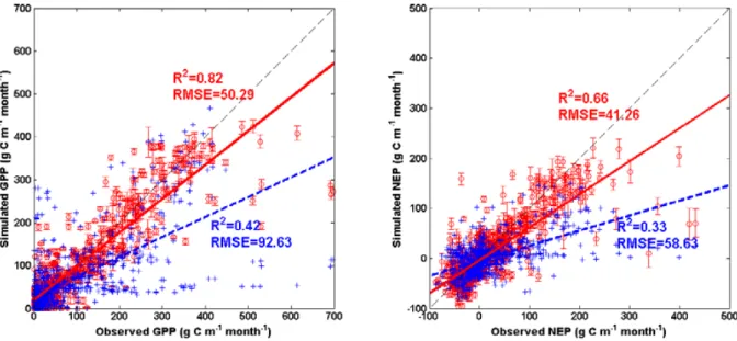
SAT-TEM estimated GPP and NEP are under- or over-predicted for some sites. The model could not capture ex-ceptionally high values in the summer at some sites, such as some summer months at the cropland sites (Bondville, Rosemount, Mead Irrigated). Underestimations of NEP also take place in the winters at the Howland site, the springs and the winters at the Wind River Crane site, possibly due to the overestimation of the ecosystem respirations at these two sites. The model also overestimated GPP at the Varia Ranch site in winters. Considering the low quality of GPP in winters (most of them<0), our estimation could still be in a reasonable range. If we pool all the measured fluxes together (Fig. 4), SAT-TEM shows better performance.
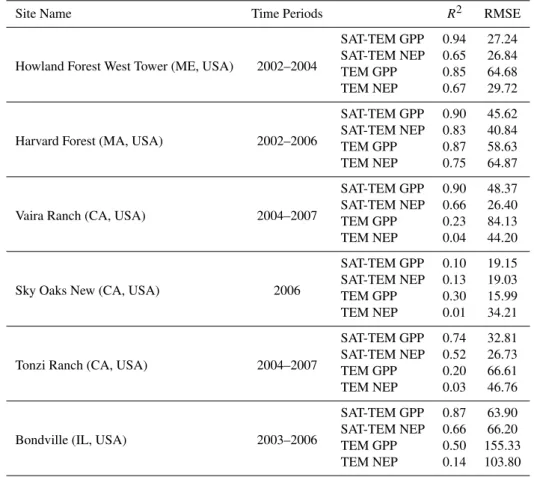
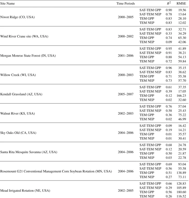
Table 4.Statistical results for the observed and SAT-TEM and TEM predicted monthly GPP and NEP at each AmeriFlux site for parameter-ization. The units of RMSE are g C m−2month−1.
Site Name Time Periods R2 RMSE
Howland Forest West Tower (ME, USA) 2002–2004
SAT-TEM GPP 0.94 27.24
SAT-TEM NEP 0.65 26.84
TEM GPP 0.85 64.68
TEM NEP 0.67 29.72
Harvard Forest (MA, USA) 2002–2006
SAT-TEM GPP 0.90 45.62
SAT-TEM NEP 0.83 40.84
TEM GPP 0.87 58.63
TEM NEP 0.75 64.87
Vaira Ranch (CA, USA) 2004–2007
SAT-TEM GPP 0.90 48.37
SAT-TEM NEP 0.66 26.40
TEM GPP 0.23 84.13
TEM NEP 0.04 44.20
Sky Oaks New (CA, USA) 2006
SAT-TEM GPP 0.10 19.15
SAT-TEM NEP 0.13 19.03
TEM GPP 0.30 15.99
TEM NEP 0.01 34.21
Tonzi Ranch (CA, USA) 2004–2007
SAT-TEM GPP 0.74 32.81
SAT-TEM NEP 0.52 26.73
TEM GPP 0.20 66.61
TEM NEP 0.03 46.76
Bondville (IL, USA) 2003–2006
SAT-TEM GPP 0.87 63.90
SAT-TEM NEP 0.66 66.20
TEM GPP 0.50 155.33
TEM NEP 0.14 103.80
3.2 Temporal variation of carbon fluxes in the
conterminous US
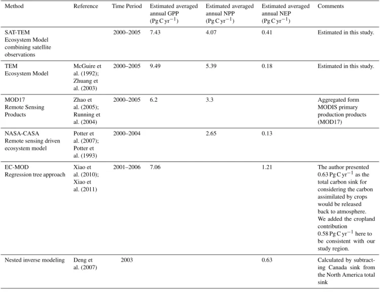
Annual GPP, NPP and NEP for the conterminous United States over the period 2000–2005 vary from year to year (Table 6). Discrepant results are found comparing to pre-vious studies in the same region and similar time period (Ta-ble 7). The SAT-TEM estimated GPP flux varies from 7.02 to 7.78 Pg C yr−1with of an annual average 7.43 Pg C yr−1. This estimate is close to 7.06 Pg C yr−1 estimated by Xiao et al. (2010) over the period 2001–2006 but higher than 6.2 Pg C yr−1of MODIS GPP product (Zhao et al., 2005) for the period of 2000–2005. Our estimate NPP ranges from 3.81 to 4.38 Pg C yr−1in this period, which is much higher than the range of 2.67–2.79 Pg C yr−1over 2000–2004 from Potter et al. (2007) and the 3.3 Pg C yr−1from MODIS NPP product over 2000–2005 (Zhao et al., 2005). Our estimated NEP is 0.08–0.73 Pg C yr−1with an average 0.41 Pg C yr−1. Overall our estimations are higher than 0.04–0.2 Pg C yr−1 from Potter et al. (2007), and much lower than the estimates as high as 1.21 Pg C yr−1from Xiao et al. (2011) but our es-timation of 0.40 Pg C yr−1in 2003 is closer to the estimate of
0.63 Pg C yr−1based on an inverse modeling approach (Deng et al., 2007). Comparing to NEP in the 1980s, SAT-TEM estimated a much higher sink than the VEMAP estimate, which put the sink as 0.08±0.02 Pg C yr−1, and the land-based analyses (0.08–0.35 Pg C yr−1)(Turner et al., 1995; Houghton et al., 1999, 2000), but close to the results (0.30– 0.58 Pg C yr−1)provided by Pacala et al. (2001).
2000 2001 2002 2003 2004 2005 -20 0 20 40 60 80 100 120 140 160 180 Year GP P (g C m o n th -1)
2000 2001 2002 2003 2004 2005 -60 -40 -20 0 20 40 60 80 Year NEP (g C m o n th -1) (a)
2000 2001 2002
0 50 100 150 200 250 300 Year G P P( g C m ont h -1)
2000 2001 2002
-40 -20 0 20 40 60 80 100 Year NEP (g C m o n th -1) (b)
2001 2002 2003 2004 2005 2006 -100 0 100 200 300 400 500 Year G P P( g C m ont h -1)
2001 2002 2003 2004 2005 2006 -150 -100 -50 0 50 100 150 200 250 Year N E P( g C m ont h -1) (c)
2000 2001 2002 2003
-50 0 50 100 150 200 250 300 350 400 450 Year G P P( g C m ont h -1)
2000 2001 2002 2003
-100 -50 0 50 100 150 200 250 Year NEP (g C m o n th -1) (d)
Fig. 3.Comparison of seasonal variations of the observed GPP and NEP with SAT-TEM and TEM predictions at the ten additional AmeriFlux sites. Dashed lines are the observed values while circles and crosses are the predictions with SAT-TEM and TEM, respectively. The error bars indicates the standard deviation of the results by ensemble SAT-TEM simulations with 50 sets of posterior parameters:(a)Niwot Ridge site;(b)Wind River Crane site(c)Morgan Monroe State Forest site;(d)Willow Creek site;(e)Kendall Grassland site;(f)Walnut River site;
(g)Sky Oaks Old site;(h)Santa Rita Mesquite Savanna site;(i)Rosemount G21 Conventional Management Corn Soybean Rotation site;
2005 2006 2007 -50 0 50 100 150 200 250 300 Year G P P( g C m ont h -1)
2005 2006 2007
-60 -40 -20 0 20 40 60 80 Year NEP (g C m o n th -1) (e)
2000 2001 2002 2003
-50 0 50 100 150 200 250 300 350 400 450 Year G P P( g C m ont h -1)
2000 2001 2002 2003
-100 -50 0 50 100 150 200 250 Year NEP (g C m o n th -1) (f)
2004 2005 2006
-20 0 20 40 60 80 100 120 Year G P P( g C m ont h -1)
2004 2005 2006
-60 -40 -20 0 20 40 60 80 Year NEP (g C m o n th -1) (g)
2004 2005 2006
-20 0 20 40 60 80 100 120 Year G P P( g C m ont h -1)
2004 2005 2006
-60 -40 -20 0 20 40 60 80 Year NEP (g C m o n th -1) (h)
2004 2005 2006 -100
0 100 200 300 400 500 600 700
Year
G
P
P
(g C
m
ont
h
-1)
2004 2005 2006
-100 -50 0 50 100 150 200 250 300 350 400
Year
N
E
P
(g C
m
ont
h
-1)
(i)
2002 2003 2004 2005
-100 0 100 200 300 400 500 600 700
Year
G
P
P(
g
C
m
ont
h
-1)
2002 2003 2004 2005
-100 0 100 200 300 400 500
Year
NEP
(g
C m
o
n
th
-1)
(j)
Fig. 3.Continued.
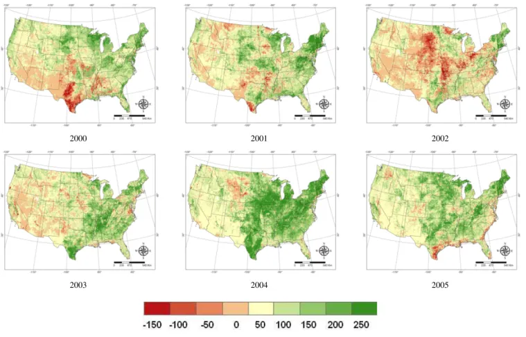
area which is very likely due to cool or cold weather of the highland climate, temperature changes and extreme droughts might be the reason causing the other large area of car-bon sources in these years. The National Climatic Data Center (NCDC, http://www.ncdc.noaa.gov/oa/ncdc.html) re-ported that the contiguous US was very warm during the summer but very cold in November and December in 2000. Southwest states such as Utah, New Mexico and Nevada ex-perienced the second or the third warmest year on record. Apart from the abnormal temperature, the drought in 2000 severely affected much of the southern and western US and therefore reduced the carbon uptake and enhanced the in-tensity of carbon source. In 2001, the Midwest and Pacific Southwest both had abnormally high temperatures. 2003 was reported as the 20th warmest year on record for the United States. Western regions were reported as much warmer than average for the summer. The Northwest Region had its sec-ond warmest summer on record, and the Southwest and West had their third in 2003. Abnormally high air temperature significantly enhances ecosystem respirations but does not contribute much to carbon uptake because the temperature may have passed the range of optimums temperature for plant photosynthesis during the summer time. Consequently, the ecosystem acts as a low sink or becomes a carbon source. Year 2002 had the lowest GPP, NPP and NEP during this period. 2002 was an extreme drought year, in which pre-cipitation was lower than 30-yr mean annual value. As the year began, moderate to extreme drought covered one-third
of the contiguous United States including much of the eastern seaboard and northwestern United States. The combination of generally warmer- and drier-than-average conditions led to a large area of carbon source in 2002 (Fig. 5). In addition to the limitations of the carbon uptake, the extreme drought also significantly enhanced the respiration and therefore led to a more severe carbon source. These results suggest that the use of EVI and LSWI is able to reflect the real large-scale environmental conditions and to constrain the estimates of carbon fluxes.
In contrast, the year 2004 had slightly above-average tem-peratures and was the 6th wettest year on record of the nation (NCDC 2004). The year 2005 was above-average warm but had much lower than average temperatures along the Eastern Seaboard in growing season and the precipitation was near the long-term mean of precipitation in the nation (NCDC 2005). These climate patterns resulted in a high sink in these 2 yr and a carbon source in the eastern regions in 2005.
Table 5.Statistics for the observed and SAT-TEM and TEM predicted monthly GPP and NEP at each AmeriFlux site for parameterization. The units of RMSE are g C m−2month−1.
Site Name Time Periods R2 RMSE
Niwot Ridge (CO, USA) 2000–2005
SAT-TEM GPP 0.90 19.56
SAT-TEM NEP 0.78 13.64
TEM GPP 0.83 28.10
TEM NEP 0.83 12.02
Wind River Crane site (WA, USA) 2000–2002
SAT-TEM GPP 0.83 32.71
SAT-TEM NEP 0.33 34.29
TEM GPP 0.74 65.30
TEM NEP 0.09 42.06
Morgan Monroe State Forest (IN, USA) 2001–2006
SAT-TEM GPP 0.95 41.89
SAT-TEM NEP 0.91 38.21
TEM GPP 0.88 54.13
TEM NEP 0.72 59.84
Willow Creek (WI, USA) 2000–2003
SAT-TEM GPP 0.96 35.15
SAT-TEM NEP 0.83 38.62
TEM GPP 0.71 55.38
TEM NEP 0.73 57.70
Kendall Grassland (AZ, USA) 2005–2007
SAT-TEM GPP 0.61 37.35
SAT-TEM NEP 0.39 17.05
TEM GPP 0.12 166.23
TEM NEP 0.02 32.60
Walnut River (KS, USA) 2002–2003
SAT-TEM GPP 0.76 57.04
SAT-TEM NEP 0.58 25.43
TEM GPP 0.36 75.22
TEM NEP 0.02 46.99
Sky Oaks Old (CA, USA) 2004–2006
SAT-TEM GPP 0.09 16.42
SAT-TEM NEP 0.19 14.21
TEM GPP 0.01 35.57
TEM NEP 0.01 30.41
Santa Rita Mesquite Savanna (AZ, USA) 2004–2006
SAT-TEM GPP 0.68 24.78
SAT-TEM NEP 0.12 20.59
TEM GPP 0.50 21.87
TEM NEP 0.03 22.78
Rosemount G21 Conventional Management Corn Soybean Rotation (MN, USA) 2004–2006
SAT-TEM GPP 0.69 93.04
SAT-TEM NEP 0.56 55.58
TEM GPP 0.51 138.89
TEM NEP 0.27 73.11
Mead Irrigated Rotation (NE, USA) 2002–2005
SAT-TEM GPP 0.66 128.83
SAT-TEM NEP 0.29 105.89
TEM GPP 0.56 180.60
TEM NEP 0.26 116.52
a carbon source into a sink earlier than the other years. Ac-cumulative NEP started to decrease in September for all of the years except 2005, which continued to assimilate more carbon than that was released in October and then reverted to a source. The early-beginning and late-ending growing
Fig. 4.Scatterplots of the observed GPP and NEP versus SAT-TEM and TEM predictions at the selected AmeriFlux sites. Black dashed lines show a 1:1 relationship. Circles and crosses, red and blue regression lines are SAT-TEM and TEM simulated values, respectively. The error bars indicates the standard deviation of the results by ensemble SAT-TEM simulations with 50 sets of posterior parameters.(a)and(b)are the predicted GPP and NEP versus observed values, respectively.
Table 6. Estimated annual GPP, NPP and NEP across conterminous United States over 2000–2005. The units of the carbon fluxes are Pg C yr−1.
Year GPP NPP NEP
SAT-TEM TEM SAT-TEM TEM SAT-TEM TEM
2000 7.24±0.33 8.85 3.85±0.63 4.87 0.33±0.18 −0.31
2001 7.35±0.35 9.32 4.06±0.63 5.27 0.41±0.17 0.02
2002 7.02±0.34 9.38 3.81±0.62 5.32 0.08±0.17 0.18
2003 7.44±0.35 10.11 4.12±0.65 5.86 0.40±0.17 0.70
2004 7.75±0.34 8.96 4.38±0.65 4.96 0.73±0.18 −0.19
2005 7.78±0.35 10.35 4.20±0.69 6.04 0.53±0.18 0.69
Average 7.43±0.34 9.49 4.07±0.65 5.39 0.41±0.18 0.18
The seasonality of the regional net carbon uptake can be explained by the satellite-observed vegetation indices. The monthly regional averaged EVI and LSWI vary from year to year (Fig. 6b, c). EVI generally indicates the greenness of the land surface vegetation and shows the pattern of vegetation green-up and senescence. The patterns of regional averaged EVI were similar for the 6 yr but the year 2002 had lower EVI during the green-up period in the spring and the year 2000 had relatively lower EVI during the senescent season. The lower EVI of these two years were reflected by the rel-atively low NEP in these two years. Particularly, since 2002 was the lowest-sink year, our result may suggest that abnor-mal EVI in the green-up season led to a stronger influence on the annual total NEP. In contrast, EVI of the year 2004 and 2005 were mostly higher than that of the other years,
Table 7.Comparison of carbon fluxes between TEM estimated and other existing estimates in the conterminous United States.
Method Reference Time Period Estimated averaged annual GPP (Pg C yr−1)
Estimated averaged annual NPP (Pg C yr−1)
Estimated averaged annual NEP (Pg C yr−1)
Comments
SAT-TEM Ecosystem Model combining satellite observations
2000–2005 7.43 4.07 0.41 Estimated in this study.
TEM
Ecosystem Model
McGuire et al. (1992); Zhuang et al. (2003)
2000–2005 9.49 5.39 0.18 Estimated in this study.
MOD17 Remote Sensing Products
Zhao et al. (2005); Running et al. (2004)
2000–2005 6.2 3.3 Aggregated form
MODIS primary production products (MOD17) NASA-CASA
Remote sensing driven ecosystem model
Potter et al. (2007); Potter et al. (1993)
2000–2004 2.65 0.13
EC-MOD
Regression tree approach
Xiao et al. (2010); Xiao et al. (2011)
2001–2006 7.06 1.21 The author presented
0.63 Pg C yr−1as the total carbon sink for considering the carbon assimilated by crops would be released back to atmosphere. We added the cropland contribution
0.58 Pg C yr−1here to be consistent with our study region.
Nested inverse modeling Deng et al. (2007)
2003 0.63 Calculated by
subtract-ing Canada sink from the North America total sink
Regional estimations between SAT-TEM and TEM dif-fer greatly. The averaged difdif-ferences are more than 2 and 1.4 Pg C yr−1for GPP and NPP, respectively. NEP of SAT-TEM is 0.23 Pg C yr−1 higher than that of TEM. The sim-ulated interannual variations between these two versions of TEM are also different. Specifically, SAT-TEM indicated the annual carbon fluxes increased in 2000 and 2001 and dropped to the lowest values in 2002, then kept increasing in the following years and reached the peak values in 2004 and 2005. In contrast, TEM suggested the highest and lowest GPP and NPP occurred in 2005 and 2000, respectively, and the highest NEP in 2003. During these years, TEM might over- or underestimate the water stress and PAR absorption of the vegetation and therefore made different carbon seques-tration estimations. However, the more accurate information of the land surface from satellites improves the SAT-TEM simulations. SAT-TEM’s performance also benefits from the way of parameterization using the monthly eddy fluxes while TEM was calibrated using annual fluxes only.
3.3 Spatial variation of carbon fluxes in the conterminous US
SAT-TEM simulated annual carbon fluxes generally capture the expected spatial patterns (Fig. 7). GPP and NPP have a similar spatial variability from west to east across the con-terminous United States. The West Coast, which is dom-inated by evergreen forest, has high annual GPP and NPP. The western Great Plains and the Rocky Mountain as well as the Southwest regions have relatively low GPP and NPP owing to sparse vegetation and arid climate. Cropland areas in the Midwest have relatively high GPP and NPP probably due to ample irrigation and fertilization. Highest GPP and NPP occur in the east United States with dense vegetation. The Gulf Coast has especially high GPP mainly due to its favorable temperature and abundant precipitation.
2000 2001 2002
2003 2004 2005
Fig. 5. Annual average SAT-TEM estimated NEP across the conterminous United States for each year in 2000–2005. Positive values represent carbon sink while negative values represent carbon source. Units are g C m−2yr−1.
regions in the eastern United States and especially in the Northeast with intensive radiation, abundant precipitation, warm temperature or dense vegetation cover. But the carbon sources also take place in forest regions, mostly in the south Rocky Mountain area and Sierra Nevada Mountain mainly due to the cold and dry climate. Non-forest regions includ-ing grassland, savannas, shrubland as well as cropland act as a carbon sink. Except the year 2000, most area of grassland in the south especially in Texas is a persistent carbon sink with warm weather and abundant precipitation with 100 to 250 g C m−2yr−1over the 6-yr period. Most cropland areas are carbon sinks with the intensity of 50 to 100 g C m−2yr−1. Carbon dynamics vary in different ecosystems (Table 8). Cropland contributes the most to the conterminous United States carbon sink with the highest GPP, NPP and NEP. Forests follow cropland to have high total GPP, NPP and con-tribute about one-third of the total net carbon uptake. With the second largest area, grasslands contribute about one-sixth to one-fifth of total annual GPP and NPP, and one-sixth of total annul NEP. Shrubland has the lowest total annual GPP, NPP while savannas have the lowest total annual NEP. On a per-unit area basis, forests have the highest GPP,
follow-ing with cropland and savannas. Deciduous forests have the highest NPP intensity while shrubland and grasslands have the lowest. Deciduous forest NEP is the highest and shrub-land have the lowest carbon sink. Overall, deciduous forests and croplands are the main contributors to the national car-bon sink over the period 2000–2005.
Since the disturbance damages to vegetation can be re-flected by the variations of EVI, use of EVI in TEM helps capture the effects of disturbances on carbon dynamics. For example, the Hurricane Katrina occurred in late August 2005 and affected five million acres of forest across Mississippi, Louisiana and Alabama with downed trees, snapped trunks and broken limbs to stripped leave. Dramatic changes of EVI occurred in the following two months (September and October) after the hurricane in that region. For the most in-fluenced region between 90◦W∼88◦W and 29◦N∼31◦N,
1 2 3 4 5 6 7 8 9 10 11 12 -1
-0.5 0 0.5 1 1.5
M
o
n
th
ly A
ccu
m
u
lat
ed
N
E
P
(P
g
C
) (a)
2000 2001 2002 2003 2004 2005
1 2 3 4 5 6 7 8 9 10 11 12 0.1
0.2 0.3 0.4 0.5
M
o
nt
hl
y
E
V
I
(b)
1 2 3 4 5 6 7 8 9 10 11 12 0.1
0.2 0.3 0.4 0.5
Month
M
o
n
thl
y
LSW
I
(c)
Fig. 6.Comparison between NEP, EVI, and LSWI across the con-terminous United States over the period of 2000–2005:(a) Cumu-lative monthly NEP estimated by SAT-TEM.(b)Monthly averaged regional EVI.(c)Monthly averaged regional LSWI.
abundant water storage in that period. Our SAT-TEM results agree with the findings suggesting Hurricane Katrina had large impacts on the regional carbon budget based on satellite data and empirical approaches (Chambers et al., 2007; Xiao et al., 2010).
3.4 Possible uncertainties
The data used to drive SAT-TEM and the parameterization both result in uncertainties to our estimation. As indicated by Zhao et al. (2006), the NCEP reanalysis data overestimated solar radiation and underestimated temperature. The errors in temperature may introduce errors in carbon fluxes because of the nonlinear relationship between temperature and plant maintenance respiration. The heterogeneity of land covers is another important source of uncertainty when we scale the site-level parameterization to the region. For example, C3 and C4plants in the regional simulations are not treated dif-ferently since there is no transient spatially-explicit C3 and C4plant distribution data.
Second, carbon dynamics are uncertain due to lacking spatially-explicit forest stand age data. In this study, we as-sume that all ecosystems (e.g. forests) are mature. Parame-ters generated at the chosen matured forest at Howland and Harvard forest sites do not work for young forests. Thus models may underestimate NPP of the forest in the contermi-nous United States because the forest productivity generally decreases with stand age (McMurtrie et al., 1995). Although the usage of MODIS vegetation indices can represent some information of the forest age (Waring et al., 2006), more ade-quate quantification of the regional carbon fluxes should use spatially-explicit data of forest stand age.
Third, the uncertainty came from a limited number of quality ecosystem sites. For example, there are only a few shrubland sites with sufficient observations. The weak con-straint on parameters of SAT-TEM for shrubland may bias the results. In addition, more sites in the western US should be established. The significant uncertainties of eddy flux data (Richardson et al., 2008) and the uncertainties introduced by the gap-filling techniques (Moffat et al., 2007) may also bias parameterization and regional results.
(a) GPP
(b) NPP
(c) NEP
Fig. 7. Average annual carbon fluxes (g C m−2yr−1)(left) and the relative standard deviations (right) of the conterminous United States
over the period 2000–2005:(a)GPP;(b)NPP;(c)NEP. The relative standard deviations are calculated by dividing standard deviations by the average values of the regional results of the 50 sets of simulations.
4 Conclusions
We incorporate MODIS EVI and LSWI into a process-based biogeochemistry model TEM to more adequately quantify ecosystem carbon dynamics from 2000 to 2005 for the con-terminous United States. Multiple eddy flux tower data are used to parameterize and verify the SAT-TEM. Ensemble
Table 8.TEM estimated annual carbon fluxes for each vegetation type in the conterminous United States during 2000–2005.
Vegetation Type Total Annual GPP (Pg C yr−1)
Total Annual NPP (Pg C yr−1)
Total Annual NEP (Pg C yr−1)
Mean Annual GPP
(kg Cm−2yr−1)
Mean Annual NPP kg Cm−2yr−1
Mean Annual NEP kg Cm−2yr−1
Land Area (km2)
Evergreen Forest 1.50 0.57 0.038 1.46 0.55 0.037 1 028 790
Deciduous Forest 1.28 0.95 0.110 1.53 1.13 0.131 838 203
Grassland 1.31 0.83 0.075 0.75 0.48 0.043 1 745 960
Shrubland 0.25 0.08 0.015 0.18 0.06 0.011 1 355 240
Savannas 0.39 0.27 0.012 1.34 0.93 0.041 290 155
Cropland 2.85 1.45 0.178 1.25 0.63 0.078 2 287 000
(a) EVI anomalies (b) SAT-TEM estimated GPP anomalies
(c) TEM estimated GPP anormalies
4.38 Pg C yr−1and NEP ranges from 0.08 to 0.73 Pg C yr−1 in the region during the period 2000–2005. The param-eterization introduces 0.34, 0.65 and 0.18 Pg C yr−1 errors to the regional GPP, NPP and NEP, respectively. The ef-fects of extreme climate and disturbances such as severe drought in 2002 and Hurricane Katrina in 2005 are cap-tured in our regional simulations. This study takes advan-tage of process-based ecosystem modeling, satellite obser-vations and eddy flux tower carbon flux data to provide a more adequate quantification of carbon fluxes for the conter-minous United States. Our findings and carbon flux prod-uct should benefit studies of carbon-climate feedbacks and facilitate policy-making of carbon management and climate change.
Acknowledgements. We acknowledge the AmeriFlux community to provide the eddy flux data and the MODIS research community to provide MODIS data on vegetation. This research is supported by NSF through projects of ARC-0554811 and EAR-0630319 and the Department of Energy. The study is also supported by NASA land-use and land-cover change program. Computing support is provided by the Rosen Center for Advanced Computing at Purdue University.
Edited by: U. Seibt
References
Aalto, T., Ciais, P., Chevillard, A., and Moulin, C.: Optimal de-termination of the parameters controlling biospheric CO2fluxes
over Europe using eddy covariance fluxes and satellite NDVI measurements, Tellus B, 56, 93–104, 2004.
AmeriFlux Network, published at: http://ameriflux.ornl.gov/, 2009. Baldocchi, D., Falge, E., Gu, L., Olson, R., Hollinger, D., Run-ning, S., Anthoni, P., Bernhofer, C., Davis, K., Evans, R., Fuentes, J., Goldstein, A., Katul, G., Law, B., Lee, X., Malhi, Y., Meyers, T., Munger, W., Oechel, W., Paw, K. T., Pile-gaard, K., Schmid, H. P., Valentini, R., Verma, S., Vesala,
T., Wilson, K., and Wofsy, S.: FLUXNET: A New Tool
to Study the Temporal and Spatial Variability of Ecosystem-Scale Carbon Dioxide, Water Vapor, and Energy Flux Densi-ties, B. Am. Meteorol. Soc., 82, 2415–2434, doi:10.1175/1520-0477(2001)082<2415:FANTTS>2.3.CO;2, 2001.
Boles, S. H., Xiao, X., Liu, J., Zhang, Q., Munkhtuya, S., Chen, S., and Ojima, D.: Land cover characterization of Temperate East Asia using multi-temporal VEGETATION sensor data, Remote Sens. Environ., 90, 477–489, 2004.
Braswell, B. H., Sacks, W. J., Linder, E., and Schimel, D. S.: Esti-mating diurnal to annual ecosystem parameters by synthesis of a carbon flux model with eddy covariance net ecosystem exchange observations, Glob. Change Biol., 11, 335–355, 2005.
Canadell, J. G., Mooney, H. A., Baldocchi, D. D., Berry, J. A., Ehleringer, J. R., Field, C. B., Gower, S. T., Hollinger, D. Y., Hunt, J. E., Jackson, R. B., Running, S. W., Shaver, G. R., Stef-fen, W., Trumbor, S. E., Valentini, R., and Bond, B. Y.: Car-bon metabolism of the terrestrial biosphere: A multitechnique approach for improved understanding, 2, Springer, New York, NY, ETATS-UNIS, 2000.
Chambers, J. Q., Fisher, J. I., Zeng, H., Chapman, E. L., Baker, D. B., and Hurtt, G. C.: Hurricane Katrina’s Car-bon Footprint on U.S. Gulf Coast Forests, Science, 318, 1107, doi:10.1126/science.1148913, 2007.
Clark, K. L., Gholz, H. L., Moncrieff, J. B., Cropley, F., and Loescher, H. W.: Environmental Controls over Net Exchanges of Carbon Dioxide from Contrasting Florida Ecosystems, Ecol. Appl., 9, 936–948, 1999.
Clark, K. L., Gholz, H. L., and Castro, M. S.: Carbon dynamics along a chronosequence of slash pine plantations in north florida, Ecol. Appl., 14, 1154–1171, doi:10.1890/02-5391, 2004. Cook, B. D., Davis, K. J., Wang, W., Desai, A., Berger, B. W.,
Teclaw, R. M., Martin, J. G., Bolstad, P. V., Bakwin, P. S., Yi, C., and Heilman, W.: Carbon exchange and venting anomalies in an upland deciduous forest in northern Wisconsin, USA, Agr. Forest Meteorol., 126, 271–295, 2004.
Coops, N. C., Waring, R. H., and Landsberg, J. J.: Assess-ing forest productivity in Australia and New Zealand usAssess-ing a physiologically-based model driven with averaged monthly weather data and satellite-derived estimates of canopy photosyn-thetic capacity, Forest Ecol. Manage., 104, 113–127, 1998. Coulter, R. L., Pekour, M. S., Cook, D. R., Klazura, G. E., Martin,
T. J., and Lucas, J. D.: Surface energy and carbon dioxide fluxes above different vegetation types within ABLE, Agr. Forest Me-teorol., 136, 147–158, 2006.
Deng, F., Chen, J. M., Ishizawa, M., Yuen, C.-W., Mo, G., Higuchi, K., Chan, D., and Maksyutov, S.: Global monthly CO2flux in-version with a focus over North America, Tellus B, 59, 179–190, 2007.
Falk, M., Wharton, S., Schroeder, M., Ustin, S., and U, K. T. P.: Flux partitioning in an old-growth forest: seasonal and interan-nual dynamics, Tree Physiol., 28, 509–520, 2008.
Fan, S., Gloor, M., Mahlman, J., Pacala, S., Sarmiento, J., Takahashi, T., and Tans, P.: A Large Terrestrial Carbon Sink in North America Implied by Atmospheric and Oceanic Carbon Dioxide Data and Models, Science, 282, 442–446, doi:10.1126/science.282.5388.442, 1998.
Field, C. B., Randerson, J. T., and Malmstr¨om, C. M.: Global net primary production: Combining ecology and remote sensing, Remote Sens. Environ., 51, 74–88, 1995.
Goward, S. N. and Huemmrich, K. F.: Vegetation canopy PAR ab-sorptance and the normalized difference vegetation index: An assessment using the SAIL model, Remote Sens. Environ., 39, 119–140, 1992.
Green, E. J., MacFarlane, D. W., Valentine, H. T., and Strawder-man, W. E.: Assessing Uncertainty in a Stand Growth Model by Bayesian Synthesis, Forest Sci., 45, 528–538, 1999.
Griffis, T. J., Sargent, S. D., Baker, J. M., Lee, X., Tanner, B. D., Greene, J., Swiatek, E., and Billmark, K.: Direct mea-surement of biosphere-atmosphere isotopic CO2exchange using the eddy covariance technique, J. Geophys. Res., 113, D08304, doi:10.1029/2007jd009297, 2008.
Guenther, B., Xiong, X., Salomonson, V. V., Barnes, W. L., and Young, J.: On-orbit performance of the Earth Observing Sys-tem Moderate Resolution Imaging Spectroradiometer; first year of data, Remote Sens. Environ., 83, 16–30, 2002.
T., Maksyutov, S., Masarie, K., Peylin, P., Prather, M., Pak, B. C., Randerson, J., Sarmiento, J., Taguchi, S., Takahashi, T., and Yuen, C.-W.: Towards robust regional estimates of CO2sources
and sinks using atmospheric transport models, Nature, 415, 626– 630, 2002.
Hazarika, M. K., Yasuoka, Y., Ito, A., and Dye, D.: Estimation of net primary productivity by integrating remote sensing data with an ecosystem model, Remote Sens. Environ., 94, 298–310, 2005. Hollinger, D. Y., Goltz, S. M., Davidson, E. A., Lee, J. T., Tu, K., and Valentine, H. T.: Seasonal patterns and environmental con-trol of carbon dioxide and water vapour exchange in an ecotonal boreal forest, Glob. Change Biol., 5, 891–902, 1999.
Hollinger, D. Y., Aber, J., Dail, B., Davidson, E. A., Goltz, S. M., Hughes, H., Leclerc, M. Y., Lee, J. T., Richardson, A. D., Ro-drigues, C., Scott, N. A., Achuatavarier, D., and Walsh, J.: Spa-tial and temporal variability in forest-atmosphere CO2exchange, Glob. Change Biol., 10, 1689–1706, 2004.
Hollinger, S. E., Bernacchi, C. J., and Meyers, T. P.: Carbon bud-get of mature no-till ecosystem in North Central Region of the United States, Agr. Forest Meteorol., 130, 59–69, 2005. Houghton, R. A. and Hackler, J. L.: Changes in Terrestrial Carbon
Storage in the United States. 1: The Roles of Agriculture and Forestry, Global Ecol. Biogeogr., 9, 125–144, 2000.
Houghton, R. A., Hackler, J. L., and Lawrence, K. T.: The U.S. Carbon Budget: Contributions from Land-Use Change, Science, 285, 574–578, doi:10.1126/science.285.5427.574, 1999. Houghton, R. A., Hackler, J. L., and Lawrence, K. T.: Changes in
Terrestrial Carbon Storage in the United States. 2: The Role of Fire and Fire Management, Global Ecol. Biogeogr., 9, 145–170, 2000.
Huete, A., Liu, H. Q., Batchily, K., and van Leeuwen, W.: A com-parison of vegetation indices over a global set of TM images for EOS-MODIS, Remote Sens. Environ., 59, 440–451, 1997. Huete, A., Didan, K., Miura, T., Rodriguez, E. P., Gao, X., and
Fer-reira, L. G.: Overview of the radiometric and biophysical perfor-mance of the MODIS vegetation indices, Remote Sens. Environ., 83, 195–213, 2002.
Iman, R. L. and Helton, J. C.: An Investigation of Uncertainty and Sensitivity Analysis Techniques for Computer Models, Risk Anal., 8, 71–90, 1988.
IPCC: Climate Change 2001: Synthesis Report. A Contribution of Working Groups I, II, and III to the Third Assessment Report of the Intergovernmental Panel on Climate Change, edited by: Watson, R. T. and the Core Writing Team, Cambridge University Press, Cambridge, United Kingdom and New York, NY, 2001. Justice, C. O., Townshend, J. R. G., Vermote, E. F., Masuoka, E.,
Wolfe, R. E., Saleous, N., Roy, D. P., and Morisette, J. T.: An overview of MODIS Land data processing and product status, Remote Sens. Environ., 83, 3–15, 2002.
Kistler, R., Collins, W., Saha, S., White, G., Woollen, J., Kalnay, E., Chelliah, M., Ebisuzaki, W., Kanamitsu, M., Kousky, V., van den Dool, H., Jenne, R., and Fiorino, M.: The NCEP-NCAR 50-Year Reanalysis: Monthly Means CD-ROM and Documen-tation, B. Am. Meteorol. Soc., 82, 247–267, doi:10.1175/1520-0477(2001)082<0247:TNNYRM>2.3.CO;2, 2001.
Law, B., Turner, D., Campbell, J., Lefsky, M., Guzy, M., Sun, O., Tuyl, S., and Cohen, W.: Carbon fluxes across regions: observa-tional constraints at multiple scales, in: Scaling and Uncertainty Analysis in Ecology: Methods and Applications, edited by: Wu,
J., Jones, K. B., Li, H., and Loucks, O. L., Columbia University Press, New York, 167–190, 2006.
Li, Z., Yu, G., Xiao, X., Li, Y., Zhao, X., Ren, C., Zhang, L., and Fu, Y.: Modeling gross primary production of alpine ecosystems in the Tibetan Plateau using MODIS images and climate data, Remote Sens. Environ., 107, 510–519, 2007.
Lipson, D. A., Wilson, R. F., and Oechel, W. C.: Effects of Elevated Atmospheric CO2on Soil Microbial Biomass, Activity, and
Di-versity in a Chaparral Ecosystem, Appl. Environ. Microbiol., 71, 8573–8580, doi:10.1128/aem.71.12.8573-8580.2005, 2005. Lu, X. and Zhuang, Q.: Evaluating climate impacts on carbon
bal-ance of the terrestrial ecosystems in the Midwest of the United States with a process-based ecosystem model, Mitigation and Adaptation Strategies for Global Change, 15, 467–487, 2010. Ma, S., Baldocchi, D. D., Xu, L., and Hehn, T.: Inter-annual
vari-ability in carbon dioxide exchange of an oak/grass savanna and open grassland in California, Agr. Forest Meteorol., 147, 157– 171, 2007.
McGuire, A. D., Melillo, J. M., Joyce, L. A., Kicklighter, D. W., Grace, A. L., Moore III, B., and Vorosmarty, C. J.: Interactions Between Carbon and Nitrogen Dynamics in Estimating Net Pri-mary Productivity For Potential Vegetation in North America, Global Biogeochem. Cy., 6, 101–124, doi:10.1029/92gb00219, 1992.
McGuire, A. D., Sitch, S., Clein, J. S., Dargaville, R., Esser, G., Foley, J., Heimann, M., Joos, F., Kaplan, J., Kicklighter, D. W., Meier, R. A., Melillo, J. M., Moore III, B., Pren-tice, I. C., Ramankutty, N., Reichenau, T., Schloss, A., Tian, H., Williams, L. J., and Wittenberg, U.: Carbon Balance of the Terrestrial Biosphere in the Twentieth Century: Analyses of CO2, Climate and Land Use Effects With Four
Process-Based Ecosystem Models, Global Biogeochem. Cy., 15, 183– 206, doi:10.1029/2000gb001298, 2001.
McMurtrie, R. E., Gower, S. T., and Ryan, M. G.: Forest Produc-tivity: Explaining Its Decline with Stand Age, Bulletin of the Ecological Society of America, 76, 152–154, 1995.
Melillo, J. M., McGuire, A. D., Kicklighter, D. W., Moore, B., Vorosmarty, C. J., and Schloss, A. L.: Global climate change and terrestrial net primary production, Nature, 363, 234–240, 1993. Moffat, A. M., Papale, D., Reichstein, M., Hollinger, D. Y.,
Richardson, A. D., Barr, A. G., Beckstein, C., Braswell, B. H., Churkina, G., Desai, A. R., Falge, E., Gove, J. H., Heimann, M., Hui, D., Jarvis, A. J., Kattge, J., Noormets, A., and Stauch, V. J.: Comprehensive comparison of gap-filling techniques for eddy covariance net carbon fluxes, Agr. Forest Meteorol., 147, 209–232, 2007.
Monson, R. K., Turnipseed, A. A., Sparks, J. P., Harley, P. C., Scott-Denton, L. E., Sparks, K., and Huxman, T. E.: Carbon sequestra-tion in a high-elevasequestra-tion, subalpine forest, Glob. Change Biol., 8, 459–478, 2002.
Myneni, R. B., Hoffman, S., Knyazikhin, Y., Privette, J. L., Glassy, J., Tian, Y., Wang, Y., Song, X., Zhang, Y., Smith, G. R., Lotsch, A., Friedl, M., Morisette, J. T., Votava, P., Nemani, R. R., and Running, S. W.: Global products of vegetation leaf area and frac-tion absorbed PAR from year one of MODIS data, Remote Sens. Environ., 83, 214–231, 2002.