Credit borrowing constraints in a DSGE framework: income vs. housing

FUNDAÇÃO GETULIO VARGAS ESCOLA DE ECONOMIA DE SÃO PAULO

DANIELA CUNHA DE LIMA

CREDIT BORROWING CONSTRAINTS IN A DSGE

FRAMEWORK: INCOME VS. HOUSING

DANIELA CUNHA DE LIMA

CREDIT BORROWING CONSTRAINTS IN A DSGE

FRAMEWORK: INCOME VS. HOUSING

Dissertação apresentada à Escola de Economia de São Paulo da Fundação Getulio Vargas, como requisito para obtenção do título de Mestre em Economia

Campo de Conhecimento: Macroeconomia

Orientador: Prof. Dr. Vladimir K.Teles

DANIELA CUNHA DE LIMA

CREDIT BORROWING CONSTRAINTS IN A DSGE

FRAMEWORK: INCOME VS. HOUSING

Dissertação apresentada à Escola de Economia de São Paulo da Fundação Getulio Vargas, como requisito para obtenção do título de Mestre em Economia

Campo de Conhecimento: Macroeconomia

Orientador: Prof. Dr. Vladimir Kuhl Teles

Data de Aprovação:

/ /

Banca examinadora:

Prof. Dr. Vladimir Kuhl Teles (Orientador) FGV-EESP

Prof. Dr. Bernardo Guimarães FGV-EESP

AGRADECIMENTOS

Ao professor Vladimir Teles, pela orientação. Aos professores Bernardo Guimarães, Luis Araújo e Ricardo Brito pelos valiosos comentários e sugestões na qualifi-cação e na defesa.

Aos professores da EESP, pelos ensinamentos desde a graduação. Ao Gustavo Arruda, por importantes contribuições a este trabalho.

Aos amigos que fiz na EESP, pela genuína contribuição e companhia nos dias infindáveis na biblioteca e fora dela.

ABSTRACT

Credit market in Brazil distinguishes from advanced economies in many aspects. One of them is related to collaterals for households borrowing. This work proposes a DSGE frame-work, based on Gerali et al.(2010), to analyse one pecularity of Brazillian credit market: payroll-deducted personal loans. To original model, we added the possibility to households contract long term debt and compare to differents types of credit constrains: one based on housing and other based on future income. We callibrate and estimate the model to Brazil, using Bayesian technique. Results show that, in a economy where credit constraints are based on income, responses to shocks appear to be stronger, at first, but dissipate faster. This occurs because income responds quickly to shock than housing prices, so does amount available to loans. In order to smooth consumption, agents compensate lower income and borrowing by increasing working hours, restoring loans and debt in a shorter time.

RESUMO

O mercado de crédito brasileiro se diferencia em diversos pontos dos mercados em econo-mias avançadas, com relação à composição do crédito, prazo médio, dentre outros. Uma dessas divergências refere-se ao colateral. Neste sentido, este trabalho propõe um modelo DGSE, com base no arcabouço desenvolvido por Gerali et al. (2010) para analisar uma peculiaridade do mercado de crédito brasileiro, o crédito consignado. Ao modelo original, acrescentamos a possibilidade de indivíduos se endividaram e analisamos dois tipos de re-strição ao crédito: uma com base na renda futura esperada outra com base no patrimônio imobiliário do agente. Nós calibramos e estimamos Bayesianamente o modelo para a econo-mia brasileira. Os resultados mostram a reação ao choque na econoecono-mia cujo crédito se baseia na renda parece ser mais intensa e se dissipar mais rapidamente do que na economia com base em housing. Isso decorre do fato de que a renda responde mais rapidamente a choques do que os preços de imóveis, e, dessa forma, a oferta de crédito consignado também.

Contents

1 Introduction 9

2 Literature Review 10

3 Model 12

3.1 Patient Households . . . 12

3.2 Impatient Households . . . 13

3.3 Entrepreneurs . . . 14

3.4 Capital and final goods producers . . . 15

3.5 The labor market . . . 15

3.6 Loan and deposit demand . . . 16

3.7 Banks . . . 18

3.7.1 Wholesale branch . . . 19

3.7.2 Retail branch . . . 20

3.8 Monetary policy and market clearing . . . 22

4 Estimation 22 4.1 Data and sources . . . 23

4.2 Calibrated parameters and Prior distributions . . . 23

5 Model Properties 26 5.1 Monetary shock . . . 27

5.2 Technology shock . . . 28

1

Introduction

The relationship between financial sector and “real economy” is well known by governments and central bankers. Troubles in banking sector frequently have significant impact in real economic activity. Although this interaction has been present in academic discussion, most of quantitative models used to focus on the demand side of credit market, as Bernanke, Gertler and Gilchrist (1999). Recent papers though studying of condition from supply side, such as degree of competition in banking sector, constraints in banks’ balance sheet, solidness of banking system, gain importance.

Despite all progress made, most of work has been focus on developed economy. Never-theless, credit market in emerging economies is different from the advanced ones. In Brazil, credit to GDP is relative low, when compared to developed economies and to world average, although it has doubled in the past decade. Another difference concerns the collateral. In developed economies, households uses their houses as collaterals in loans, but in Brazil this is uncommon, considering the dificult in retrieve this type of collateral in case of default, among others institutional and juridical reasons. When offering credit, banks evaluate in-come as a proxy to households’ wealth and its capacity of repayment. In fact, according to Brazilian Central Bank, only 30% of nonearmarked loans have some kind of collateral. These lack of collaterals contribute to lowers loans terms and wider spreads in Brazillian economy.

Our work embraces this discussion by adapting the framework developed by Geraliet al. (2010) to Brazilian economy, which is characterized by a monopolistic competitive banking sector. We believe that this framework can suit an emerging economy, with adjustments. Arruda (2013) modified the above-mentioned model by using one year of expected wages as collaterals to households’ loans.

loans. We estimate the model using Bayesian techniques and study impulse responses to monetary policy and technology shocks.

The rest of the paper is organized as follows: Section 2 reviews literature regarding finan-cial friction in DSGE models, section 3 describes the model. Section 4 presents calibration and estimation of parameters. Section 5 analyze model properties, studying monetary and technology shocks. Section 6 concludes.

2

Literature Review

Although literature regarding DSGE models with financial frictions is not exactly new, there was a lot of improvement since Bernanke, Gertler and Gilchrist (BGG, 1999). Recently works aim to develop a more complex financial sector, adding imperfect competition, risk overexpose, credit crunch among others. Cúrdia and Woodford (2008) developed a DSGE framework considering the role of credit spreads in monetary policy. Back in late 2007, Federal Reserve decrease interest rate despite the fact traditional Taylor’s rule (Taylor 1993) recommend not to. Obviously, the central banker was considering others indicators, which were already signaling problems in financial system. One of these indicators was credit spreads. With this in mind, Cúrdia and Woodford (2008) considered a modified Taylor rule for interest rate to incorporate an indicator of financial conditions: credit spreads. The model is based on heterogeneous agents, differing from impatience rate, which create a social need for financial intermediation. Others works also propose a modify Taylor rule, as Taylor (2008) and McCulley and Toloui (2008), suggesting that policy maker should adjust intercept term of Taylor rule to incorporate increase in credit spreads.

Gertler and Kiyotaki (2010) show how disruption in financial intermediation can affect real economy. Different from BGG and earlier literature, financial friction in Gertler and Kiyotaki focus on financial intermediation, in a perfect competition banking sector, not on credit constraint faced by non-financial borrowers. As in BGG, they endogenize financial market friction introducing agency problem between lenders and borrows. The authors developed a framework to incorporate at banking sector the new unconventional measures that took place during 2008 crisis. Gertler and Karadi (2011) proposed a framework in which banking sector faces endogenous balance sheet constraints to evaluate the effect of unconventional monetary policy. Results show that benefits of a central bank intervention are positive during a crisis when banks face a tightening on balance sheet constraints. The benefits are even larger when zero lower bond is reached by the nominal interest rate.

monetary policy shock. Gerali et al. (2010) incorporate imperfectly competitive banking sector and sticky rates on financial friction DSGE model. Loans to households and firms are constrained by the value of the collateral, which is given by the expected value of house-hold’s housing, similar to Iacoviello (2005) and, in case of entrepreneurs, by holding capital. Banking sector faces imperfect competition in both sides of balance sheet. Bank’s capital is accumulated out of retained earnings. They show that banking sector in a imperfect competition attenuates monetary policy shocks, mainly due to sticky rates.

Andrés and Arce (2012) also consider an imperfectly competitive banking sector, in which households are lenders and entrepreneurs borrowers. Different from Gerali et al. (2010), they do not consider interest rate rigidity nether endogenous lending margins. It’s shown that, a stronger banking competition increases output in the long run, by leading to a “reallocation of available collateral towards investors”.

Works studding emerging markets are not numerous. It’s worth to mention Gertler, Gilchrist and Natalucci (2007) who developed a small open economy macroeconomic model where financial conditions influence aggregate behavior. It exalts the important role financial accelerator mechanism had on Korean economy, accounting for about 50% of the total reduction in economic activity. Credit market frictions magnify the drop in investment demand during the crisis.

For Brazilian economy, the Central Bank of Brazil developed a complex DSGE model named SAMBA, by de Castro et at. (2011), which incorporates important features of Brazilian economy, such as fiscal rule, regulated prices, among others. But it misses to specify a banking sector structure into the model.

Kornelius (2011) adapt Gertler and Karadi (2011) framework to Brazilian economy, incorporating compulsory requirements and a shock in depositor’s trust, allowing banking run. Results showed that compulsory requirements amplify monetary policy shocks. On the other hand, compulsory requirements bring economy to a worst steady state, with lower level of capital, investment, consumption, employment, and product. Martins and Sales (2010) developed a sudden stop model DSGE model for Brazil, considering a small open economy, in which the main innovation is the imperfect credit market framework, one domestic and other international. They illustrated that it is a welfare improvement a central bank’s supply of credit directly to exporters, as long as it uses reserves to fund it. They also show that there are some good reasons to intervening in credit market, such as avoiding bank run.

3

Model

We developed a DSGE model based the framework presented by Gerali et al. (2010), incorporating some characteristics of Brazilian credit market.

The economy is composed by a unit mass of households and entrepreneurs (E). There are two groups of households; patient (P) and impatient (I), differing by discount factor. Patients households discount factor (βt

p) are higher than impatients’ (βIt) and entrepreneurs (βt

E) discount’s factor. Household works, consume and accumulate capital (deposits). En-trepreneurs hire workers; buy capital from capital-goods producer and produces homogenous intermediate goods. Patient households own firms and banks. Households offer differenti-ated labor to unions. Besides entrepreneurs, there are a monopolistically competitive retail sector and capital producers (both owned by entrepreneurs).

Heterogeneity in discounts factor induces a social need for financial intermediation. Banking sector is characterized by a monopolistic competition. Banks supply only two types of financial products: one-period savings contracts and multi-period borrowing con-tracts, which differs from a one period borrowing contract represented in Gerali et. al. (2010) and in Arruda (2013), so impatient households accumulate debt. Interest rates on loans and deposits are set in order to maximize profits.

Deposits are received from patient households and impatient households and entrepreneurs borrow a positive amount – which are financed by deposits and bank capital (accumulated out of profits). Loans are constrained by physical capital, in case of entrepreneurs. For households, we will study two types of credit constrain: one based on theirs housing stocks, as Gerali et al.(2010) and other based on the expected value of 48 month of future income.

3.1

Patient Households

Each patient household (i) maximize:

E0

∞

X

t=o

βPt

"

1−aPεztlog

cPt(i)−a P

cPt−1

+εhtlogh P t(i)−

lP t (i)1+φ

1 +φ

#

(1) In which cP

t(i) represents current individual consumption, cPt aggregate consumption,

hP

t(i) housing services,lPt (i) hours worked,aP a habit consumption coefficient andφrepresents the inverse of the Frisch elasticity. Households’ preference are subject to two kinds of shocks:εz

t, a disturbance that affects consumption and εht, affecting housing demand1 . Bud-1_{Both disturbance follow an AR(1) process type, asε}

t= (1−ρǫ)ε+ρǫεt−1+η

ǫ

t, whereε is the steady

get constraints in real terms sets:

cpt(i) +qth∆h p

t(i) +dt(i)≤w p tl

p t +

1 +rd t−1

dt−1(i)

πt

+tpt (2)

Where expenditure, consumption (cpt(i)), housing investment at priceqht and deposits (dt(i))) are financed by labor income (wtpl

p

t(i)),w p

t represents hourly real wage for patient household,

πt=Pt/Pt−1 is gross inflation) by last period deposits increased by interest deposit rates (rdt) and transfers lump-sum tpt2.

3.2

Impatient Households

As in patient households, impatient agent (i) objective is to maximize the expected utility:

E0

∞

X

t=o

βt I

"

1−aI

ǫz tlog

cI

t(i)−ac I t−1

+εh tlogh

I t(i)−

lI t(i)1+φ

1 +φ

#

(3) Subject to3_:

cI

t(i) +q h t∆h

I t(i) +

(1 +rbH

t−1)debtt−1(i)

πt

≤wI tl

I

t(i) +debtt(i) +t I

t(i) (4) Where cI

t represents impatient households consumption,rtbH borrowing interest rate,wIt impatient hour wage, lI

t work hours of impatient, tIt(i) lump-sum transfers, which includes only net union fees. Since impatient households borrow from banks, it is imposed a credit borrowing constrain. In original model, Gerali et al. (2010) credit borrowing constrain are based on households’ house stock, represented as:

(1 +rbH

t )bIt ≤mIHt Et

qh

t+1hIt(i)πt+1

−debtt (5)

Where bI

t represents households’ real borrowing. However, we will also consider a credit borrowing constrain based on expectation of future income, as below, and compare these two types of constrain, calling Benchmark (BK) the model with credit constrain based on households’ house stock and IN the model with credit constrain based on future income.

2_{Transfers lump-sum are given by dividends received from banks and entrepreneurs and labor union}

membership net fee.

3_{We can calculate this budget constrain by considering that, each period, besides consumption,}

house-holds has to pay for installments and interest. So budget constrain is cI t(i) +

rbH t₋₁debt(i)

πt +

φddebtt₋₁(i)

πt ≤

wI

tlIt(i) +bt(i) +tIt(i), wherebt represents real borrowing. Considering law of motion of outstanding debt

(eq.21) set here in real terms: debtt=bt+(1−

φd)debtt₋₁

πt ,bt=debtt−

(1−φd)debtt₋₁

πt , we can rewrite budget

constrain ascI

t(i) +qht∆hIt(i) +

(1+rbH

t₋₁)debtt₋₁(i)

πt ≤w

I

(1 +rbH

t )bIt ≤mIIt Et

 

12

X

j=1

wt+jltI+j(i)πt+j



−debt_t (6)

Where mIH

t ǫ(0,1) represents loan-to-value ratio (LTV) for credit constrains based on housing stock and mII

t ǫ(0,1) represents future income that is available for borrowing, net from current debt. So, excluding households current debt (debtt),mI

t determines the amount of credit that each household has available, considering it’s housing stocks or income. Debt structure will be fully explained in section 3.6.

3.3

Entrepreneurs

Symmetric to households, each firm (i) seek to minimize the difference between current individual and lagged consumption and maximize the following utility expectation:

E0

∞

X

t=o

βt E

"

1−aE

εz tlog

cE

t(i)−ac E t−1

− l

E t (i)1+φ

1 +φ

#

(7) Subject to:

cEt (i)+w P t l

E,P t +wItl

E,I t +

(1 +rbE

t−1)bEt−1(i)

πt

+qKt k E

t +ψ(ut(i))k E t−1 =

yE t (i)

χt

+bEt (i)+q K

t (1−δ)k E t−1

(8) Where qK

t is the price of one unit of physical capital,bEt is firm’s loans at rate rtbE ,

ψ(ut(i)) is the real cost associate to using the levelut of capacity utilization,χt≡ _PPtw t is the relative price of wholesale produced good, which is given by the following technology:

yE

t (i) =aEt [ktE−1(i)ut(i)]α[ltE(i)]1−α (9) Total factor productivity is represented by aE

t and labor lEt is a composition of patient and impatient household’s labor, aslE

t = (l E,P t )µ(l

E,I

t )1−µ. Similar to impatient households, entrepreneurs’ borrowings are constrained by physical capital, as:

(1 +rbE t )b

E t ≤m

E t Et

h

qK

t+1πt+1(1−δ)ktE(i)

i

(10) Where mE

3.4

Capital and final goods producers

Capital producer firms are perfectly competitive and owned by entrepreneurs. Firms use undepreciated (1− δ)kt−1 capital sold by entrepreneurs at price Qkt and it units of final goods, sold by retailers at price Pt to increase effective capital stock xt and sell back to entrepreneurs at price Qk

t. Capital producers maximize the follow expected utility:

E0

∞

X

t=o ΛE

0,t

qK

t ∆xt−it

(11) Subject to:

xt =xt−1+

 1−

κi 2

itεqKt

it−1

!2

i_t (12)

Where qk t ≡

Qk t

PT is the real price of capital, ∆xt =kt−(1−δ)kt−1, κi is the adjustment cost of capital creation, εqKt is an efficiency shock on investment.

On the other hand, retail sector is assumed to be in a monopolistic competition. Retailers buy intermediation goods at pricePw

t and differentiated it at no cost. Final good is sold at pricePt(j), which incorporates a mark-up. Prices at retail sector are sticky and are chosen by the following maximization:

E0

∞

X

t=o ΛP

0,t



Pt(j)yt(j)−P_twyt(j)−

κp 2

Pt(j)

Pt−1(j)

−πtlp−1π1−lp

!2

Ptyt



 (13)

Subject to consumption demand:

yt(j)≡ Pt(j)

Pt

!−εy_t

yt (14)

Where κp is the adjustment cost parameter in case retailers want to set its price beyond indexation rule andεyt represents the stochastic demand price elasticity.

3.5

The labor market

E0

∞

X

t=o

βt s

  

UCS t(i,m)

 

Ws t(m)

Pt

ls

t(i, m)−

κw 2

Ws t(m)

Ws t−1(m)

−πlw t−1π1−lw

!2 Ws t Pt  − ls

t(i, m)1+φ 1 +φ

   (15) Subject to: ls

t(i, m) =l s t(m) =

Ws t(m)

Ws t−1(m)

!−εl_t

ls

t (16)

In equilibrium, labor supply of patient household (s) - and symmetrically for household (m) - is given by:

κw

πws t −π

lw t−1π1−lw

πws

t =βsEt

  λs t+1 λs t κw

πws

t+1−πtlw−1π1−lw

πw

S t+1

πt+1

!2

+ (1−εI t)l

S t +

εl

t(lst)1+φ

ωs tλst

 

(17) Where ωs

t represents real wage for type (s) and πw s

t nominal wage inflation.

3.6

Loan and deposit demand

Loans and deposits contracts bought by households and entrepreneurs represent a basket of slight differential financial product supplied by a branch of j-banks. The elasticity of substitution terms are stochastic, which are represented by εbH

t >1 (impatient households loans), εbE

t > 1 (entrepreneurs loans) and εdt <−1 (patient households deposits), so bank spreads can move independently of monetary policy. Demand for real loans (bI

t) of household i is given by:

min_{bI t(i,j)}

1

ˆ

0

rbHt b I

t(i, j)dj (18)

Subject to:    1 ˆ 0

bI_{(i, j)} εbH

t−1

εbH t dj    εbH_t εbH t−1

≥bI

t (19)

Where rbH t =

h_´1

0 r

bH t (j)1−ε

bH t dj

i 1

1−εbH_t represents the interest rate on household’s loans.

bI t(j) =

rbH t (j)

rbH t

!−εbH_t

bI

t (20)

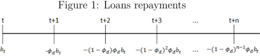
In original paper, Geraliet al. (2010) consider deposits and loans as one periods contracts. Since we’re analysing multi-period credit constrains for impatients agents, based expected future income, borrowing contracts for households will be represented as a multi-period contracts. In Brazil, noneamarked loans have an average maturity of 48 months. Deposits ans loans to firms remains one period contracts. Debt structure is model as Fortali and Lambertini (2013). In every period t, each household i take a new loan, bI

t(i), constrained by its future income. Amortization rate from the second period onwards is represented by

φdǫ(0,1). The law of motion of impatient household (i)’s outstanding debt is given by:

debtt(i) = (1−φd)debtt−1(i) +bIt(i) (21) So current debt, debtt, is represented by outstanding debt in the beginning of the period,

debtt−1, excluded current amortization4, plus new loans. Loans repayments can be illustrated

by following:

Figure 1: Loans repayments

Since impatient household takes loans each period t, current debt can be represented by:

debtt=bIt + (1−φd)bIt−1+ (1−φd)2bIt−2+ (1−φd)3bIt−3+...

debtt=bIt + (1−φd)debtt−1

Entrepreneurs’ demand for loans at bank j is represented by:

bE t (j) =

rbE t (j)

rbE t

!−εbE_t

bE

t (22)

On the deposit side, demand for real deposits (dP

t) of patient household i, it’s obtained by maximizing:

max_{dP t (i,j)}

1

ˆ

0

rd t(i, j)d

P

tdj (23)

Subject to:

   1 ˆ 0 dP t(i, j)

εd t−1

εd t dj    εd_t εd

t−1

≤dP

t (24)

Aggregate demand for deposit at bank j is given by:

dP t(j) =

rd t(j)

rd t

!−εd_t

dt (25)

Where dtrepresents aggregate deposits of the economy and rd

t is the average deposit interest rate.

rdt =

   1 ˆ 0

rdt(j)1− εd tdj    1 1₋εd

t

(26)

3.7

Banks

The main contribution in Geraliet al. (2010) is that banking sector structure is characterized by imperfect competition at retail level, which reflects Brazilian credit market. In 2013, four’s biggest bank concentrates 75% of deposits5_.

Banks has market power to set interest rates on deposits and loans in response to shocks. All financial intermediation is done exclusive by banks. In other words, banks receive all deposits and supply loans to impatient households and entrepreneurs. Every bank must meet the following identity:

Bt =Dt+Ktb (27) Each individually j bank must use its deposits Dt and/or its bank capital Ktb to finance overall loans Bt – this two source are perfect substitutes. The proportion of deposits and bank capital is defined based on exogenous capital-to-assets level (leverage). Bank’s cap-ital is almost fixed in the short run, and it’s accumulated over retained earnings. In this framework, bank capital has an important role in setting conditions to credit supply and in economics cycle. A negative macroeconomic environment can leads to a drop in bank’s profit and capital, which may cause deterioration on credit condition, as lower loans sup-plied to private sector credit – amplifying the original contraction. Each bank j, jǫ[0,1] is composed by three parts: two “retail” branch and one “wholesale” unit. The wholesale unit is responsible for managing capital group position and retail branches are responsible

for (i) supplying differentiated loans to impatient households and entrepreneur and (ii) for receiving differentiated deposits from patient households.

3.7.1 Wholesale branch

The wholesale branch market is a perfect competition one and each wholesale’s loans (Bt) must equal wholesale’s deposits,Dt, plus bank capital (Ktb). The cost for moving away the capital-to-asset ratio (Ktb

Bt ) from target level (υ

b_{) relies on wholesale unit. Geraliet al. (2010)} set υb _{parameter at 9%. According to Brazilian Central Bank financial stability report}6 _,

Brazilian banking sector’s capital-to-asset is arround 10%. Each period, wholesale unit accumulates capital as:

πtKtb = (1−δ b₎

Ktb−1+j

b

t−1 (28)

In whichδb _{represents cost associated of managing bank capital and j}b

t−1 is overall real

profit made by the three branches. The problem of wholesale unit is to choose the amount of loans and deposits that maximizes the discounted sum of real cash flows:

max{Bt,Dt}E0

∞

X

t=o ΛP

0,t =

"

(1 +Rb

t)Bt−Bt+1πt+1+Dt+1πt+1−(1 +Rdt)Dt+ +(Kb

t+1πt+1−Ktb)−

κkb 2

Kb t

Bt

−υb

!2

Kb t



 (29)

Subject to the balance sheet Bt =Dt+Ktb . WhereRbt represents net wholesale loans rate and Rd

t net wholesale deposit rates, both are takes as given. Rearranging (27) and including the constraint twice (for t and for t+1), we can rewrite the objective function as:

max{Bt,Dt}RbtBt−RbtDt−

κkb 2

Kb t

Bt

−υb

!2

Kb

t (30)

From first order conditions we have:

Rb t =R

d t −κkb

Kb t

Bt

−υb

! Kb t Bt !2 (31) To guarantee solution, it’s assumed that banks have unlimited access to finance at policy rate rt. Considering the fact that wholesale market is a perfect competitive one, wholesale deposits rates and interbank market rate are equal: Rd

Rb

t =rt−κkb

Kb t

Bt

−υb

! Kb t Bt !2 (32) Rearranging, the spread between wholesale loans and deposits rates are given by:

Stw ≡R b

t −rt =−κkb

Kb t

Bt

−υb

! Kb t Bt !2 (33) Capital-to-asset ratio is inversely related to spread between wholesale loans and deposits rates. A higher leverage increases the spread and profits per unit of capital. But if leverage exceedsυb _{target, a quadratic cost is paid and reduces profits. First order condition imposes} that the loans rates are choose so that marginal cost of increasing leverage equals to spread.

3.7.2 Retail branch

Retail banks are monopolistic competitors and are composed by loan and deposit branch.

3.7.2.1 Loan branch The retail loan branch from each bank j obtains wholesale loans (Bt) at rate Rb

t, from wholesale unit, differentiates them at no cost and then resell them to impatient households and entrepreneurs charging different mark-ups. In order to introduce sticky rates, it is assumed that each retail bank faces a quadratic cost for changing interest loans rates. So retail loan unit maximize:

max_{rbH

t (j),rtbE(j)}E0

∞

X

t=o ΛP

0,t =

"

rtbH(j)b I

t(j) +r E t (j)b

E

t (j)−R b

tBt− (34)

−κbH

2

rbH t (j)

rbH t−1(j)

−1

!2

rbH t bIt −

κbE 2

rbE t (j)

rbE t−1(j)

−1

!2

rbE t bet

 

Subject to loans demand from impatient households and entrepreneurs:

bI t(j) =

rbH t (j)

rbH t

!−εbH_t

bI

t (35)

bE t (j) =

rbE t (j)

rbE t

!−εbE_t

bE

t (36)

WhereBt(j) =bt(j) =bI

1−εbst +ε bs t Rb t rbs t

−κbs

rbs t

rbs t−1

−1

!

rbs t

rbs t−1

!

+ (37)

+βPEt

  

λP t−1

λP t κbs rbs t+1 rbs t −1 ! rbs t+1 rbs t !2 bs t+1 bs t    = 0

WhereλP_{t represents the Lagrange multiplier for budget constraint for patient household.}

Log-linearizing (35) and assumingεb_ts=εb_{s (for a simplified case) we have:}

ˆ

rbs t =

κbs

εbs_{−1 + (1 +β} P)κbs

ˆ

rbs t−1+

βPκbs

εbs_{−1 + (1 +β} P)κbs

Etˆrbs t+1 +

+ ε

bs₋₁

εbs_{−1 + (1 +β} P)κbs

ˆ

Rbt−

ˆ

εbs t

εbs_{−1 + (1 +β} P)κbs

(38)

3.7.2.2 Deposit branch Retail deposits bank’s j unit collects patient household’s deposits,dP

t, and pass them to wholesale unit, where deposits are remunerated at rate rt. The problem of deposit unit is to maximize the following:

max_{rd t(j)}E0

∞

X

t=o ΛP

0,t =



rt(j)Dt(j)−rd_t(j)dP_t (j)−

κd 2

rd t(j)

rd t−1(j)

−1

!2

rd tdt



 (39)

Subject to household’s deposits demand:

dpt(j) =

rd t(j)

rd t

!−εd_t

dpt (40)

Where Dt(j) = dP

t (j). After imposing a symmetric equilibrium, first order condition is given by:

−1 +εdt −ε d t

rt

rd t

−κd

rd t

rd t−1

−1

!

rd t

rd t−1

+βPEt

  

λP t−1

λP t κd rd t+1 rd t −1 ! rd t+1 rd t !2

dt+1

dt

  

= 0 (41)

And assuming εd

t =εd(for a simplified case), the log-linearization version of eq. (39) is:

ˆ

rd t =

κd 1 +εd_{+ (1 +β}

P)κd ˆ

rd t−1+

βPκd 1 +εd_{+ (1 +β}

P)κd

Etˆrd t+1 +

1 +εd 1 +εd_{+ (1 +β}

P)κd ˆ

Overall real profits of a bank j are the sum of net profits from retail branches and wholesale unit, as represented below:

jb t =r

bH t b

H t +r

bE t b

E_−r tdt−

Kb t

Bt

−υb

!2

Kb

t −Adj B

t (43)

Where AdjB

t represents the adjustment cost of changing interest rates on loans and de-posits.

3.8

Monetary policy and market clearing

Central Bank sets interest ratert according to the following Taylor’s rule:

(1 +rt) = (1 +r)(1+φR)(1 +rt−1)φR

π

t

π

φπ(1−φR) y

t

yt−1

!φy(1−φR)

εrt (44) In which r is the nominal interest rate at stationary level, φRrepresents the weight of inflation deviation from the target,π,φy is the weight impute to output growth and εrt is a white noise shock, with σr as its standard deviation.

Market clearing in goods markets is given by:

yt=ct+qtk[kt−(1−δ)kt−1] +kt−1ψ(ut) +δb

Kb t−1

πt

+Adjt (45)

Where ct represents aggregate consumption, kt the aggregate stock of physical capital,

Kb

t represents aggregate bank’s capital andAdjtare all real adjustment costs, of price, wage and interest wage. In housing market, the aggregate stock is fixed,h, and equilibrium is set by: h=hP

t(i) +hIt(i).

4

Estimation

4.1

Data and sources

There were used twelve series, described below. We demeaned rates, except monetary policy rate, with were detrended, once natural rate in Brazil presents a clear downward trend during sample period. All other variables were detrended, using HP filter with smoothing parameters set at 1600.

Real consumption: final consumption of households, constant price, seasonally ad-justed. Source: IBGE, Contas Nacionais.

Real investments: gross fixed capital formation, constant price, seasonally adjusted: Source: IBGE, Contas Nacionais.

Real housing prices: proxy using civil construction deflator, real estate and rent deflator. Source: IBGE, Contas Nacionais.

Wages: proxy using real payroll and hours per worker, seasonally adjusted. Source: IBGE, BCB

Inflation: quarter over quarter log difference of IPCA. Source: IBGE

Nominal interest rate: SELIC. Source: BCB

Nominal interest rate on loans to households: proxy using noneamarked loans to households, firms, interest rate on noneamarket loans to firms and interest rate on noneam-erket loans. Source: BCB, series 8288, 3959, 3960 and 8287.

Nominal interest rate on loans to firms: rate on noneamarket loans to firms. Source: BCB, series 8288.

Nominal interest rate on deposits: weighted average interest rate on term deposits, with preset rate, post set rate and floating. Source: BCB, series 32, 33, 40,41,1167,1168,1183 and 1184.

Loans to households: noneamarket loans to households. Source: BCB, series 3960.

Loans to firms: noneamarket loans to firms. Source: BCB, series 3959.

Deposits: sum of preset, post set and floating term deposits. Source: BCB, series 33, 41,1168 and 1184.

4.2

Calibrated parameters and Prior distributions

Eighteen parameters are calibrated according to Castroet al. (2011) and Geraliet al. (2010) for Brazilian economy.

For patient household’s discount factor we consider real interest rate ex ante7 _{in analised}

period, so βP_{was set as 0.98. Impatient discount factor (β}I_{) and firm’s (β}E_{) were set 0.96,} as Gerali et al. (2010) used a 0.2 gap between patient household’s discount factor and

impatient. For inverse of the Frisch elasticity, φ, the share of unconstrained households, µ, and weight of housing in households’ utility function,εh _{we use the same values as in Gerali} et al.(2010).

Capital share of production function,α, we used 0.448 according to de Castro et al. (2011), which matches average ration capital GDP for Brazilian economy. As for depre-ciation rate of physical capital (δ = 0.015), markup in goods markets, ( εy

εy₋₁ = 10%) and markup in labor markets, ( εl

εl₋₁ = 50%), we also calibrated using de Castro et al. (2011). Regarding banking sector, parameters associated with loan-to-value ratio (LTV) for households were calibrated as following: (i) for credit constrains based on future income, we considered LTV, mII _{= 0.35, once its represents noneamarked loans to annual disposal} income in Brazilian credit market; (ii) for credit constrains based on housing, we assumed

mIH _{= 0.70, the same value as in Gerali et al. (2010). On the other hand, we set} en-trepreneurs’ LTV, mE_{, at 0.20, lower than 0.35 used in Gerali et al. (2010). Noneamarket} loans to entrepreneurs in Brazil are characterized by short term maturity, as BNDES offers long terms loans at rates bellow to market average, justifying the lower LTV as seen in original paper. Since average maturity for noneamarket credit to households in Brazil is 48 months, we calibrate the amortization rate per period, φd, at 0.0625. For banking capital-to-loan ratio,υb_{, we use 10%, according to Brazilian bank system data. At last, for banking} mark ups εbH

εbH₋₁, for households, and εbE

εbE₋₁ for entrepreneurs, and mark down, εd

εd₋₁we adjust to reflect wider spreads seen in Brazilian data. For cost for managing the bank’s capital position,δP_{, it was used the same value from Gerali et al. (2010).}

Table 1: Calibrated Parameters

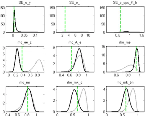
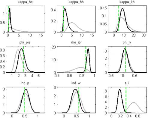
Table 3: Prior and posterior distribution of the structure parameters

5

Model Properties

We study how the transmission mechanism of monetary and technology shocks is affected in the presence of two differents credit constrains: (i) credit constrain based on households’ house stock, called Benchmark (BK) and (ii) credit constrain based on future income, called

5.1

Monetary shock

Financial intermediation has an important role in transmission of shocks: in an adverse macroeconomic environment, banks’ profits decreases and might negatively affect capital, increasing leverage, which may force banks to respond by reducing amount of loans - widen-ing the effect of the original negative shock.

Literature regarding DSGE models with financial friction and financial intermediation shows that, in an environment with perfect competition, banking sector amplifies the re-sponse on GDP due to a monetary policy shock - see Christianoet al. (2008). On the other hand, when consider imperfect competition in banking sector, it is found an attenuating effect, either with flexible rates, see Andrés e Arce (2012), or sticky rates, Gerali et al. (2010), Goodfriend and McCallum (2007). However, Gerali et al. (2010) show that this attenuating effect is mainly due to stick rates, weakening the transmission from an increase in interest rate to lending rates. In fact, they illustrate that market power in banking sec-tor has limited influence in output - once markups amplify effects for borrowers, though markdown attenuates changes for lenders.

Here, the traditional interest channel of monetary impulse come along with others, see Calza et al. (2009), (i) nominal debt: since amortization and interest payments are set in nominal terms, a fall in inflation rates redistributes resources between lenders and borrowers, (ii) credit constrain: innovation on monetary policy rate can change loan-to-value ratio, as it modify system liquidy, impacting borrowers consumption and (iii) asset-price effect, monetary policy may affect housing prices and by doing this affect the value disposal to borrowing.

Figures 2 and 3 show impulse responses to an unanticipated 50 basis points exogenous shock in monetary policy rate, rt. Overall, the direction of responses goes according to literature.

Figure 2: Impulse response function of a contractionary monetary policy shock

Figure 3: Impulse response function of a contractionary monetary policy shock

5.2

Technology shock

attenuates the response of consumption and output of a technology shock, while response of investment is widen. On the other hand, banking market power and sticky rates contributes somehow limiting and postponing shock’s transmission, as the repass for borrowing rates are done partially and slowly.

Figures 4 and 5 show responses to an one standard deviation shock at technology, aE_. Due to a fall in final good prices, here is a cut in monetary policy rate, triggering a decrease in lending rates, making loans more attractive. Investment is boost by increase in technology and also by an improvement in loans conditions. As investment rises, capital prices increases, widening even more entrepreneurs’ borrowing capacity.

Households’ credit borrowing constrain is also affected in two different ways: by an im-provement in collateral and decrease in borrowing rates. At first here is a fall in working hours, due to this increase in productive. But as labor becomes more productive, en-trepreneurs increases labor demand, amplifying wages and working hours with a lag. In IN model, collateral is boost through this channel, leading to an increase in loans and subse-quently in households’ debt. In BK model, it is also experienced a loose in credit constrains, as housing prices increases. As in monetary policy shock, we see a more volatile GDP in IN model than in BK model.

Figure 4: Impulse response function of a positive technology shock

6

Conclusion

This work has presented a DSGE model based on Geraliet al. (2010), which is character-ized by monopolistic competitive banking sector and sticky rates, with some adjustments to an emerging market economy. Brazilian credit market is quite different from the devel-oped ones. We explore divergences in the collateral in loans to households. In develdevel-oped economies, households uses their houses as collaterals in loans, but emerging economies, as Brazilian, suffer from lack of collaterals, which leads to lowers loans terms and wider spreads. The original model was modified by adapting credit constrains to impatients households ac-counting four years of expected future income and multi-period loans, so households are allowed to assume debt, which will also affect amount available to loans.

We study how this credit constrain based on income changes monetary policy and tech-nology shocks transmission compare to an identical model, with credit constrains based on housing. In order to do so, we calibrate and estimate the parameters to Brazilian economy, using Bayesian techniques. Overall, the direction of impulse responses goes according to lit-erature in both cases. Notwithstanding, the model with households’ credit constrains based on income GDP presented more volatility than the model with credit constrains based on housing. This occurs because income responds quickly to shock than housing prices, so does amount available to loans. In order to smooth consumption, agents compensate lower income and borrowing by increasing working hours, restoring loans and debt in a shorter time.

References

Andrés, J., & Arce, O. (2012). Banking Competition, Housing Prices and Macroeconomic Stability.The Economic Journal, 122(565), 1346-1372.

Arruda, G. (2013). DSGE model with banking sector for emerging economies: estimated using Bayesian methodology for Brazil. Dissertação, Escola de Economia de São Paulo, FGV.

Banco Central do Brasil. (2013). Relatório de Estabilidade Financeira.v. 12 nº2. Bernanke, B. S., Gertler, M., & Gilchrist, S. (1999). The financial accelerator in a quantitative business cycle framework.Handbook of macroeconomics, 1, 1341-1393. Calza, A., Monacelli, T., & Stracca, L. (2013). Housing finance and monetary policy. Journal of the European Economic Association, 11(s1), 101-122.

Christiano, L. J., Eichenbaum, M., & Evans, C. L. (2005). Nominal rigidities and the dynamic effects of a shock to monetary policy. Journal of political Economy, 113(1), 1-45. Christiano, L., Motto, R., & Rostagno, M. (2007). Financial factors in business cycles. Mimeo.

de Castro, M. R., Gouvea, S. N., Minella, A., dos Santos, R. C., & Souza-Sobrinho, N. F. (2011). Samba: Stochastic analytical model with a bayesian approach.Working Paper Series, 239, Banco Central do Brasil.

Cúrdia, V., & Woodford, M. (2010). Credit spreads and monetary policy. Journal of Money, Credit and Banking, 42(s1), 3-35.

Forlati, C., & Lambertini, L. (2013). Mortgage Amortization and Welfare. Job Market Paper, École Polytechnique Fédérale de Lausanne, EPFL

Gerali, A., Neri, S., Sessa, L., & Signoretti, F. M. (2010). Credit and Banking in a DSGE Model of the Euro Area.Journal of Money, Credit and Banking, 42(s1), 107-141.

Gertler, M., & Kiyotaki, N. (2010). Financial intermediation and credit policy in business cycle analysis. Handbook of monetary economics, 3(11), 547-599.

Goodfriend, M., & McCallum, B. T. (2007). Banking and interest rates in monetary policy analysis: A quantitative exploration.Journal of Monetary Economics, 54(5), 1480-1507. Iacoviello, M. (2005). House prices, borrowing constraints, and monetary policy in the business cycle.American economic review, 739-764.

Kornelius, A. (2011). Política monetária e compulsório em um modelo DSGE com fricções financeiras.Dissertação, Universidade Católica de Brasilia.

McCulley, P., & Toloui, R. (2008). Chasing the neutral rate down: Financial conditions, monetary policy, and the taylor rule.Global Central Bank Focus, 2002-2008.

Silva, G. C. D. (2013). Avaliando o mecanismo de transmissão da política monetária por meio do canal do crédito: estimação bayesiana em modelos DSGE com fricções financeiras. Tese, Universidade de Brasília

Smets, F., & Wouters, R. (2003). An estimated dynamic stochastic general equilibrium model of the euro area. Journal of the European economic association, 1(5), 1123-1175. Taylor, J. B. (1993, December). Discretion versus policy rules in practice. In Carnegie-Rochester conference series on public policy (Vol. 39, pp. 195-214). North-Holland.

Appendix

Prior and posterior marginal distribution. The marginal posterior densities are based on 10 chain, each which 100,000 draws based on the Metropolis algorithm. Black lines denote the posterior distribution and gray lines the prior distribution.