A theoretical connection between inflation and income inequality

(1)

-...---~--- - - -- - -

-P/EPGE SPE

F U N D A

ç

Ã O

GETULIO VARGAS

,~

FGV

EPGE

SEMINÁRIOS DE PESQUISA

ECONÔMICA DA EPGE

A theoretical connection between

inflation and income inequality

RUBENS PENHA CVSNE

(FGV)

Data: 15/01/2004 (Quinta-feira)

Horário: 16h

Local:

Praia de Botafogo, 190 - 11

0

andar

Auditório nO 1

Coordenação:

(2)

• A Theoretical Connection Between Inflation

and Income Inequality*

Rubens P. Cysne, Paulo K. Monteiro and Wilfredo Maldonado!

January 12, 2004

Abstract

This work investigates the effects of inflation on income distribu-tion. We use a dynamic shopping-time model to show that a differen-tiated access to transacting technologies by poor and rich consumers is enough to generate a positive link between inflation and the Gini coefficient of income distribution.

1 Introduction

Although there remains a controversy on the empirical literature relating infiation to income distribution (Galli and Hoeven (2001) call it the infiation-income inequality puzzle) several works in the area (e.g., Bulir (2001), Romer and Romer (1998» present compelling evidences that, at least for high rates of infiation, these variables are positively correlated.

This literature, though, still lacks optimizing dynamic models which de-liver such result from a theoretical perspective, formally associating infiation with some measure of income inequality. Our purpose in this paper is filling in this gap.

Elsewhere (Cysne and Maldonado (2004», we study this problem from a search-theoretic perspective. Here, instead, we concentrate on examining the

* Keywords: Inflation, Gini Coefficient, Income Inequality, Income Distribution. JEL: E40, D60

tFGV IRJ, FGV IRJ and UFF IRJ, respectively. Rubens P. Cysne thanks the hospital-ity of the Department of Economics of the Univershospital-ity of Chicago.

(3)

-•

•

possibility that a link between inflation and income distribution can be gen-erated solely by means of a differentiated access to transacting technologies. The usual connection between inflation and income distribution, regarding the different amount of inflation tax paid by richI _{and poor consumers, as}

percentage of their incomes, is kept away fram our considerations.

The shopping time chosen by the poor and by the rich differ because the latter, by assumption, have access to a better transacting technology. The underlying intuition connecting inflation to income distribution, in this case, is that the higher the rate of inflation, the more important turns out to be this lack of balance between the more and the less endowed consumers.

lndeed, when the nominal interest rate is equal to zero, both the rich and the poor have the same shopping-time, equal to zero. The higher the rate of inflation and the interest rate, though, the higher the opportunity costs of holding monetary assets, and the higher the substitution away from monetary assets to shopping time. Therefore, one should expect those with access to a better transacting technology to do relatively better when inflation is higher. We shall see that this is indeed what happens in the economy.

2 The model

Our basic model draws upon the homogeneous-agents shopping-time model with interest-bearing deposits presented by Simonsen and Cysne (2001) and Cysne (2003), which, in turn, draws upon Lucas (2000).

Our economy has an infinite number of homogenous-consumers cohorts. The cohorts are classified by the praductivity of their consumers in the pro-duction of the consumption good, and distributed in the [0,1] interval. Each cohort has the same (large) number of consumers. There are no transactions between different cohorts. The productivity of consumers in cohort j E [0,1] is Oj

>

O. We suppose that the productivity is nondecreasing in j. There is a cutoff productivity 0J'] E (0,1) such that consumers in cohorts with produc-tivity Dj

<

oJ

are called "poor" and consumers in cohorts with productivity

Oj

>

oJ

are called "rich".

The poor have access only to currency (M), which they use to make their transactions. The rich can use currency and an interest-bearing assets X to make their transactions2. X pays a nominal interest rate equal to i_{x .}The

I What we mean by rich and poor consumers is defined later in the texto

(4)

rich also buy bonds (B) form the government. Bonds pay an interest rate i and are not used for transacting.

In the description of the model, for the sake of notational clarity, we

suppress the subindex j that characterizes the (homogeneous) consumers in each cohort.

Both types of consumers, rich and poor, gain utility from the consump-tion of a single non-storable consumpconsump-tion good, and have a separable utility function

1

00

e-gtu (Ct) dt, c E

C ([O, (0), [O,

(0)). ₍₁₎ We suppose that U is continuous, increasing and concave. Consumers in each cohort are endowed with one unit of time that can be used to transact (s) ar to be used in the production of the consumption good, y, according to the production function:

y

=

8(1 - s)

₍₂₎

2.1 Government and Banks

Our economy is a Fisherian economy with lump sum taxation, where the governrnent can implement any given interest rate vector. We shall therefore refer to the nominal interest rate as a policy variable. The government, here consolidated with the Central Bank, is supposed to issue currency and bonds, and to collect reserve requirements from the banks. Banks buy bonds from the governrnent and issue X. The banking system is competitive.

k

(O

<

k

<

1) stands for the reserve requirement on X. The zero-profit

condition implies i - ix = ki.

2.2 The rich consumer maximization problem

With the price of the consumption good indicated by

P

=

P(t),

the rich consumers in each cohort j face the budget constraint:

(5)

H indicates the (exogenous) fiow of money transferred to the consumer by the government, and the dot over the variable its time derivative. Each consumer takes H as exogenous in his optimization problem.

Making 7r

=

p/

P (infiation rate) , m

=

M/ P, x = X / P and h

=

H / P, and taking into account (2), the budget constraint ofthe rich consumer (meaning, of a consumer in a cohort with productivity j

> ]) reads:

m

+

i; = ó (1 - s) - c

+

h

+

(i - 7r)b

+

(ix - 7r)x - 7rm (3)

In the steady state, the consolidation of the balances of the government and of the banks Ieads to:

(4)

Since our purpose here is concentrating on the shopping-time association between infiation and income distribution, we want to rule out the possibility that different (relative) amounts of net real financiaI income paid by each cohort interfere in the income distribution processo We do this by assuming that h is determined by the government in such a way that equation (4) holds separately for each cohort j.

Rich consumers have access to a shopping technology F (m, x, s) where m

2:

O, x

2:

0, s E [0,1] , Fm

> 0,

Fx

> 0,

Fs

> O. Further conditions on the

function

F(.)

will be introduced Iater.

The rich consumer maximizes 1 subject to (3) and to

O~c~F(m,x,s)

The first order conditions for a steady state soIution of the maximization

problem are given by: .

i=7r+g óFm

=

iFs

óFx = (i - ix)Fs

(6)

2.3 The poor consumer maximization problem

Poor consumers also have access to the technology F (m, x, s) but are not allowed to adopt it fully, since they are constrained to having x = O. The poor consumer maximizes 1 subject to

o

~ c ~

F(m,O,s)

c

+

m

~ 8 (1 - s)

+

h - 7rm The first arder condition is:

(9)

3 The Steady State Solutions

From this section onwards, we shall, when necessary, use the subindexes p and T, respectively, for poor and rich. We shall also restrict our analysis to

the case of a transacting technology weakly separable in shopping time and monetary assets, by making

F(m,x,s)

=

G(m,x)s3. G(m,x)

is differen-tiable, homogeneous of degree one, increasing with respect to each variable and with Gm/Gx an increasing function of

x/mo

• Rich:

Equations (7) and (8) now read:

iG = Gm8s kiG Gx8s

(10) (11)

In equilibrium, since the consumption good is non-storable and the gov-ernrnent transfers to each cohort match the net amount of real interests paid or received:

8(1 -

s)

= c

=

G(m, x)s.

(12)

(7)

Given the hypotheses about G(m, x), the marginal rate of substitution is an increasing function of the asset ratio x / m. Taking the inverse function and using (10) and (11):

J/C) >0 (13) Equations (10), (11) and (12), with k fixed, determine Sn m_r and _{X r} as a

function of the policy variable i :

-i (1

+

kJ (l/k))

2G (1, J

(l/k))

+

J(I/k)8sr

i (1

+

kJ (l/k)) 8sr

i (1

+

kJ (l/k))·

i2 ₍₁

₊

_{kJ (1/k))2} _i₍₁

₊

_{kJ (l/k))}

---''---'---'--.:....:,-+--'=:---;----:-~-:-7-'--4G (1, J (l/k))2 G (1, J (l/k))

This determination proceeds as follows: Since G( m, x)

=

mGm

+

xGx

(Euler's theorem), from (10) and (11):

i(

mr

+

kxr )

Sr = 8 (14)

To obtain the equilibrium variables use (13) to get X_ras a function of m_{r .} Then use (14) to get mr (and xr ) as a function of Sr. Finally, by taking into

consideration that G(m, x) = mG(I, J(I/k)), one can obtain Sr by using the

expressions for mr and Xr in (12) .

• Poor:

In this case equations (10) and (12) are still valid, however, with x = O. The first degree homogeneity.of G implies G (m, O)

=

mG (1, O) and Gm

=

(8)

Following the same procedure previously outlined, the solutions for the poor are given by:

-2 i2 _i

2G

(1, O)

+

---..." +-,---:-

4G (1,

0)2

G (1, O)

4 Main Results

Note that

sp(O)

=

sr(O)

= O, since in this case there is no private cost asso-ciated with the use of money. Lemma 1 establishes necessary and sufficient conditions for the shopping time of the poor to be greater than the shopping time of the rich.

Lemma 1 sp

>

Sr iff the transaction technology and the parameter k are

such that

G(l, J(ljk))

>

G(l,

0)(1

+

kJ(ljk))

(15)

Proof. Sr and sp are determined, respectively, as roots of the quadratic

equations:

and

f ( ) -

2 (1

+

kJ(ljk))i _

(1

+

kJ(ljk))i

r S - s

+

G(l,J(ljk))

s

G(l,J(ljk))

2 i i

fp(s)

=

s

+

G(l, O) s - G (1, O)

(16)

(17)

The family of quadratic equations

g(

x; b)

=

X2

+

bx - b, b

> O always presents

a real root Xl such that O

<

Xl

<

14. Besides, since this root satisfies

xi

+

bXI - b =

o,

it follows from the implicit function theorem that:

dXI

=

1-Xl

>

O

db y'b2

+

_4b

(9)

The demonstration is complete once one notices that (15) is equivalent to

h · (l+kJ(l(k))i i ' (16) d (17)

avmg G(l,J(l(k))

<

G(l,O) m an . •

Condition (15) is satisfied if the productivity of the transacting technology with respect to x is high enough for all values of x and m. Indeed, this enhances the disadvantage of the poor due to not having access to this asset, thereby leading them to spend more time shopping. Example 1 below shows that this condition is satisfied, for instance, when G(m, x) is a CES function with an elasticity of substitution (J

E (1,00).

• The Gini Coefficient and the Rate of Inflation

To measure the inequality in the income distribution we use the Gini coefficient of income distribution. The Gini coefficient G is given by:

G

=

1-

21

1

L(j)dj (18)

where

stands for the Lorenz curve. The Lorenz curve measures the proportion of the total income of the economy that is received by the lowest 100j% of the consumers. It can be easily shown that the Gini coefficient expresses the area between the Lorenz curve and the Lorenz curve for an economy where everyone receives the same income.

We proceed to calculate the Gini coefficient for our economy. Note that Sr

and sp do not depend on the productivity coefficient Ój. It will be notationally convenient to define

(10)

The first step is to calculate

Jt

cudu. If j

< ],

If j

>],

r

j cudu

=

t

c~du

+

~j

c:du

=

(1 - sp)

~J

+

(1 - sr)

(~j

-

~J)

.

lo

.h

Thus, from (18):

Jg

(1- sp)

~jdj

+

p

((1- sp)

~J

+

(1- sr)

(~j

-

~J))

dj

G=1-2 J

(1 - sp) ~J

+

(1 - sr) (~I

-

~J)

G

=

1 _ 2-(

l_-_sp_) --.;fJ,-+_( l_----..;.sp-;-)

-:-~_'_J

_( l-;---:-J_· )_+-:-(:-l_-_s-:-r:-) -;-:(

f_I_-_f~J"'-;-)

_-_(_1

_-_s_r )_(

l_-_])_~--,,-J

(1 - sp) ~J

+

(1 - sr) (~I

-

~J)

G = 1 _ 2 (1 - sp) (fJ

+

~J

(1 - ]))

+

(1 - sr) (f I - f] -

~J

(1 - ])) (19)

(1- sp)~J

+

(1-sr) (~I

-

~J)

Proposition 2 lf condition (15) is satisfied, then the Gini coefficient is a

non-decreasing function of the nominal interest rate (or, equivalently, of the rate of infiation), at the point i

=

O.

Proof. We proceed by calculating the derivative af the Gini coefficient with respect to the interest rate at i

=

O.

f~

+

~~ (1 - )-:)

+

fI - f~ - ~~ (1 - )-:) fI

G (O) = 1 - 2 J J J J = 1 2

-~I ~I

G(i)-G(O)

2

-~d1- sp) (fJ

+

~J (1- ])) - ~d1 - sr) (fI - fJ - ~J (1 - ]))

~I [~J (1 - sp)

+

(~I

-

~J) (1 -

Sr)]

fl~J (1 - sp)

+

fI (~I - ~]) (1 - sr)

+--7---~--~~--~

(11)

Since

rI

=

r]

+

.11

I:::.udu

<

r]

+

1:::.

₁

(1 - ])

J

we have

Therefore,

G(i) - G(O)

2

>

O Ç} sp(i)

>

sr(i)

Taking the lirnit as í --+ O,

The Proposition follows from Lemma 1. •

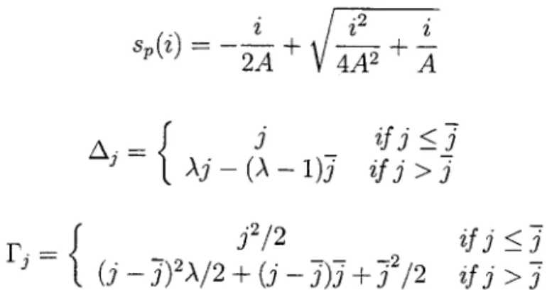
Example 1 We consider the transacting technology F(m, x, s) = G(m, x)s

=

A(ma +xa)l/a s , A

>

O, O

<

a

<

1 and productivities Ój = Ó if j ::;], Ój

=

Àó,

if j

>]

(À

>

1).

Note that in this case:

kJ(l/k)

=

ka/(a-l)

G(l, J(l/k) = A(l

+

ka/(a-l))l/a

lt can be easily checked that the condition (15) and the previous assumptions

about G are satisfied. In this case

(ó

can be taken as equal to one in the

calculations of G because it cancels out):

'2 "

Z a Z a

- ( 1

+

ka-I )2(1-1/a)

+

-(1

+

k;;-::Y)l-l/a

4A2 A

( ") z (1 k -a ) l-lia

Sr Z

= -

2A

+

a - I

+

10

(12)

• j2/2

if j ::;

J

if j

>

J

r - {

J

-(j - J)2)'/2

+

(j -

J)}

+

J2/2

if j ::;

J

if j

>

J

The value of the Gini coefficient for different values of the interest rate can be obtained using (19) and the above expressions. Table 1 presents the values of ST) sp and of the Gini coefficient for the parameter values a=0.3,

A=40, k =0.25,

J

=0. 'lf?, ).

=

10 and interest rates equal to O, 100%, 200% and 500%.

Table 1

Interest Rate(100%) O 1 2 5

Sr O 0.046 0.065 0.100

sp O 0.146 0.200 0.296 Gini Coefficient 0.5192 0.5383 0.546 0.560

Figure 1 presents the evaluation of the Gini coefficient when interest rates assume values between zero and a thousand percent.

5 Conclusions

We have developed a simplified model, based on a shopping-time rationale, to investigate the effects of inflation on the Gini coefficient of income distri-bution. A basic assumption of the model is that some (cohorts of) consumers have access to a better transacting technology than others. Our basic con-clusion is that a formal link between inflation and the Gini coefficient of income distribution based solely on this fact can be theoretically proved. For transacting technologies satisfying a certain condition, established in the text, an increase of the inflation rate unequivocally leads to a deterioration of the income distribution. Finally, we have provided an example that satisfies such condition and in which the Gini coefficient is a monotonically increasing function of the rate of inflation.

(13)

References

[1] Bulir, Ales, 2001, 1ncome 1ncome 1nequality: Does 1nfiation Matter? 1MF Staff Papers, Vol 48, n. 1.

[2J Cysne, Rubens P. (2002): "On the 1ntegrabiIity of Partial Equilibrium Measures of the WeIfare Costs of 1nfiation." Journal of Banking and Finance, 26, 12, 2357-2363.

[3] Cysne, Rubens P. (2003): "Divisia 1ndex, 1nfiation and WeIfare". Jour-nal of Money, Credit and Banking, VoI. 35, 2, 221-239

[4] Cysne, Rubens P. and MaIdonado, WiIfredo L. (2004), "Search, 1nfiation and 1ncome Distribution". Working Paper, FGV jUFF.

[5J Galli, R. and Hoeven, R., "1s infiation bad for income inequaIity: The importance of the initial rate of infiation". Working Paper, The Uni ver-sity of Lugano, Switzerland.

[6J Lucas, Robert E. Jr. "The WeIfare Costs of 1nfiation". University of Chicago working paper, (January 1993).

[7J _________ , 2000. "1nfiation and Welfare." Econometrica 68 62 (March 2000), 247-274.

[8J Mulligan, Casey B. and Xavier X. SaIa-i-Martin, 1996, Adoption of Fi-nanciaI Technologies: 1mplications for Money Demand and Monetary Policy, NBER Working Paper Series, n. 5504

[9] Romer, Christina D. and David H. Romer, 1998, Monetary Policy and the Well-Being of the Poor, NBER Working Papers Series, n. 6793. [10] Simonsen, Mario H. and Cysne, Rubens P. "WeIfare Costs of 1nfiation

(14)

.,

..

_c

4)

u

lhe Gini Coefficien! as a FuncUon of lhe Inleres! Rate

058

057

056 ~

055 o

u

'1:

~

0S4

052

0.51

L-...L~_--L...---L_-L---L--:---:--~-:'1'O O

Interest Rale

Figure 1:

13

000333900

BIBLIOTECA

MARIO HENRIQUE SIMONSEN