Março de 2015
Working
Paper
375
Household
Borrowing
Constraints
and Monetary Policy in Emerging
Economies
TEXTO PARA DISCUSSÃO 375•MARÇO DE 2015• 1
Os artigos dos Textos para Discussão da Escola de Economia de São Paulo da Fundação Getulio
Vargas são de inteira responsabilidade dos autores e não refletem necessariamente a opinião da
FGV-EESP. É permitida a reprodução total ou parcial dos artigos, desde que creditada a fonte.
Household Borrowing Constraints and Monetary Policy in
Emerging Economies
Gustavo Arruda
∗Daniela Lima
†Vladimir K. Teles
‡Abstract
Credit markets in emerging economies can be distinguished from those in advanced economies
in many respects, including the collateral required for households to borrow. This work proposes a DSGE framework to analyze one peculiarity that characterizes the credit markets of some emerging
markets: payroll-deducted personal loans. We add the possibility for households to contract long-term debt and compare two different types of credit constraints with one another, one based on housing and the other based on future income. We estimate the model for Brazil using a Bayesian technique.
The model is able to solve a puzzle of the Brazilian economy: responses to monetary shocks at first appear to be strong but dissipate quickly. This occurs because income – and the amount available
for loans – responds more rapidly to monetary shocks than housing prices. To smooth consumption, agents (borrowers) compensate for lower income and for borrowing by working more hours to repay
loans and erase debt in a shorter time. Therefore, in addition to the income and substitution effects, workers consider the effects on their credit constraints when deciding how much labor to supply, which
becomes an additional channel through which financial frictions affect the economy.
Keywords: Credit constrains, emerging markets, monetary policy. JELs: E20; E44; E51
∗Sao Paulo School of Economics - FGV †Sao Paulo School of Economics - FGV
1
Introduction
Although researchers have documented that financial frictions, in particular household borrowing
con-straints (Iacoviello, 2005; Monacelli, 2008), play a key role in business cycles, very little attention has
been paid to the heterogeneity of that friction in different countries, particularly in developing countries.
In developed economies, households use their houses as collateral for loans, but in emerging economies
this is uncommon due to the difficulty in foreclosing against this type of collateral in the event of default,
among other institutional and legal reasons. One consequence of this difficulty in collateralizing credit
is that the volume of credit that is available to households in emerging countries is much lower than in
developed countries. (In 2005, household credit represented 9.2% of GDP in emerging countries in Latin
America, 12.1% in emerging countries in Europe, and 27.5% in emerging countries in Asia; however,
household credit represented 58% of GDP in mature markets (IMF, 2006)).
Therefore, when offering credit, banks in developing countries evaluate income as a proxy for
house-hold wealth and the capacity of the househouse-hold to make repayment. A clear example of this difference
is Brazil, where the government promoted institutional changes in 2003 to diminish the risk for banks
that were introducing payroll loans. With these lines of credit, a worker’s debt service is automatically
deducted from his/her payroll check each month, reducing the risk of default. The volume of credit
ex-tended to households as a percentage of GDP has doubled since the introduction of these institutional
changes, and payroll loans now represent 70% of the volume of household credit in Brazil1.
As a result, certain aspects of the credit markets in these economies may not perform as predicted
by standard models, such as the difference in the reaction of the product to monetary policy shocks. In
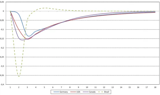
Brazil, this response is quite different from that observed in developed countries (Fig. 12), with much less
persistence, although stronger.
Differences in parameters in the Brazilian economy – including the stickiness of prices and wages,
habit formation and strategic complementarity – may explain the more severe impact of monetary policy
on the product, but there should also be greater persistence (da Silva, et al, 2012). In this paper, we solve
this puzzle by developing a model that incorporates differences in the conditions of household credit
constraints. This occurs because income – and the amount available for lending – responds more quickly
to shocks than housing prices. To smooth consumption, agents (borrowers) compensate for lower income
and for borrowing by increasing their working hours and repaying loans and debt in a shorter time.
1
Other articles studying the importance of this alternative line of credit in the behavior of agents (Costa and de Mello, 2008) or in the scheme of Brazilian macroeconomics (Carvalho et al, 2013;. Carvalho et al 2014) have proven to be important, but those models address different aspects of such loans than those covered in this article.
2The impulse response of a shock in the interest rate on the product is obtained from a VAR with 4 variables: Interest
Figure 1: Impulse response of GDP to interest rates
-0,4 -0,35 -0,3 -0,25 -0,2 -0,15 -0,1 -0,05 0 0,05
1 2 3 4 5 6 7 8 9 10 11 12 13 14 15 16 17 18
Germany USA Canada Brazil
This result provides a new channel through which financial frictions affect the economy – the choice
of labor supply by households – because the choice of labor supply now largely determines the credit
constraints to which households are subject. Thus, in a period of economic contraction, families suffer
an immediate impact on their credit restrictions, but they adjust their labor supply to compensate for
the diminished collateral. Therefore, in addition to the income and substitution effects, workers take
into account the effects on their credit constraints when deciding how much labor to supply. Somewhat
quickly (in due course), the payroll loan channel reinforces the income effect on labor supply.
We compare two kinds of credit constraints – one based on housing and other based on expected future
income – with certain adaptations. In Gerald et al (2010), loans are constrained by physical capital (in the
case of entrepreneurs) and by the expected value of housing stocks (for impatient households). We will
use the expected value of 48 months of future income because it is the average maturity of non-earmarked
resource loans to households. We also consider multi-period loans to households, instead of one-period
contracts, as in Gerali (2010), such that impatient households are allowed to accumulate debt, which suits
better conditions in the credit market, because loans are typically multi-period contract and households
are typically able to borrow fresh capital before repaying the previous loan. Existing debt will also limit
the amount available for lending. We estimate the model using Bayesian techniques to study the impulse
The rest of the paper is organized as follows: Section 2 describes the model. Section 3 presents the
calibration and estimation of parameters. Section 4 analyzes the model properties and emphasizes the
study of monetary and technology shocks. Section 5 concludes.
2
Model
We developed a dynamic stochastic general equilibrium (DSGE) model based on the framework presented
by Geraliet al. (2010) and by incorporating multi-period loans to households – instead of one-period
contracts – and a credit constraint based on future income.
The economy consists of a unit mass of households and entrepreneurs (E). There are two groups of
households that differ by discount factor: patient and impatient. Patient households’ discount factors (βtp)
are higher than those of impatient households (βt
I) and those of entrepreneurs (βEt). Households work,
consume and accumulate capital (deposits). Entrepreneurs hire workers, buy capital from producers of
capital goods and produce homogenous intermediate goods. Patient households own firms and banks.
Households offer differentiated labor to unions. In addition to entrepreneurs, there is a monopolistically
competitive retail sector and there are capital producers (both owned by entrepreneurs).
Heterogeneity in discount factors induces a social need for financial intermediation. The banking
sector is characterized by monopolistic competition. Banks supply only two types of financial products:
one-period savings contracts and multi-period borrowing contracts – which differs from the one-period
borrowing contract represented in Gerali et. al. (2010) – such that impatient households accumulate debt.
Interest rates on loans and deposits are set to maximize profits.
Deposits are received from patient households and impatient households, and entrepreneurs borrow
a positive amount, which is financed by deposits and bank capital (accumulated from profits). Loans
to entrepreneurs are constrained by physical capital. For households, we will study two types of credit
constraints: one based on their housing stocks, as in Gerali et al.(2010), and the other based on the
expected value of 48 months of future income.
2.1
Patient Households
Each patient household (i) maximizes as follows:
E0
∞ X
t=o
βPt
1−aP
εztlog c P
t (i)−a P
cPt−1
+εhtlogh P t (i)−
lP t(i)1+φ
1 +φ
(1)
in which cP
housing services,lP
t (i)is hours worked,aP is a habit consumption coefficient, andφrepresents the inverse
of the Frisch elasticity. Households’ preferences are subject to two types of shocks:εz
t, a disturbance that
affects consumption, andεh
t, affects housing demand3. Budget constraints in real terms set the following:
cpt(i) +q h t∆h
p
t(i) +dt(i)≤wptl p t +
1 +rd t−1
dt−1(i)
πt
+tpt (2)
where expenditure, consumption (cpt(i)), housing investment at price qht and deposits (dt(i)) are
fi-nanced by labor income (wtpltp(i));wpt represents hourly real wage for patient households;πt=Pt/Pt−1 is
gross inflation) by last period deposits increased by interest deposit rates (rd
t) and lump-sum transferst p t4.
2.2
Impatient Households
As with patient households, impatient agent (i)’s objective is to maximize expected utility:
E0
∞ X
t=o
βt I
1−aI
ǫz
tlog cIt(i)−acIt−1
+εh
tloghIt(i)−
lI t(i)1+φ
1 +φ
(3)
subject to the following5:
cI
t(i) +q h t∆h
I t(i) +
(1 +rbH
t−1)debtt−1(i)
πt
≤wI tl
I
t(i) +debtt(i) +tIt(i) (4)
where cI
t represents impatient households consumption: rbHt is the borrowing interest rate; wIt is
the impatient hour wage;lI
t represents the work hours of impatient; and tIt(i)is the lump-sum transfers,
which includes only net union fees. Because impatient households borrow from banks, a credit borrowing
constraint is imposed. In the original model, Geraliet al. (2010) credit borrowing constraints are based
on households’ housing stock, represented as follows:
(1 +rbH t )b
I t ≤m
IH
t Et qht+1hIt(i)πt+1
−debtt (5)
wherebI
t represents households’ real borrowing. However, we will also consider a credit borrowing
constraint based on the expectation of future income, as below, and compare these two types of
con-3Both disturbances follow an AR(1) process type, as inε
t= (1−ρǫ)ε+ρǫεt−1+ηtǫ, whereεis the steady state value and
ηǫ
t˜i.i.dN(0, σ2).
4Lump-sum transfers are calculated by dividends received from banks and entrepreneurs, in addition to labor union
mem-bership net fees.
5We can calculate this budget constraint by considering that each period, in addition to consumption, households must
pay for installments and interest. Thus, the budget constraint iscI t(i) +
rbH t−1debt(i)
πt +
φddebtt−1(i)
πt ≤w
I
tlIt(i) +bt(i) +tIt(i), wherebtrepresents real borrowing. Considering the law of motion of outstanding debt (eq.21) set here in real terms,debtt=
bt+(1−
φd)debtt−1
πt ,bt=debtt−
(1−φd)debtt−1
πt , we can rewrite the budget constraint asc
I
t(i)+qth∆hIt(i)+
(1+rtbH−1)debtt−1(i)
πt ≤
wI
strains with one another, calling the model with the credit constraint based on households’ house stock
Benchmark (BK), and the model with the credit constraint based on future income is called theINmodel.
(1 +rbHt )b I t ≤m
II t Et
12
X
j=1
wt+jltI+j(i)πt+j
!
−debtt (6)
wheremIH
t ǫ(0,1)represents loan-to-value ratio (LTV) for credit constraints based on housing stock
andmII
t ǫ(0,1) represents the future income that is available for borrowing, net of current debt. Thus,
excluding households current debt (debtt), mIt determines the amount of credit that each household has
available, considering its housing stock and/or income. Debt structure will be fully explained below, in
section 3.6.
2.3
Entrepreneurs
Symmetric with households, each firm (i) seeks to minimize the difference between current individual
and lagged consumption and to maximize the following utility expectation:
E0
∞ X
t=o
βt E
1−aE
εz
tlog cEt (i)−acEt−1
−l E t (i)1+φ
1 +φ
(7)
subject to:
cEt (i)+w P t l
E,P t +w
I tl
E,I t +
(1 +rbE
t−1)bEt−1(i)
πt
+qtKk E
t +ψ(ut(i))ktE−1 =
yE t (i)
χt
+bEt (i)+q K
t (1−δ)k E t−1 (8)
whereqK
t is the price of one unit of physical capital,bEt , represents firm’s loans at ratertbE , ψ(ut(i))
is the real cost associated with using the levelutof capacity utilization, andχt ≡ PPwt
t is the relative price
of a produced good at wholesale, which is given by the following technology:
yE
t (i) =a E t [k
E
t−1(i)ut(i)]α[ltE(i)]
1−α (9)
Total factor productivity is represented byaE
t and laborlEt is a combination of patient and impatient
households’ labor, aslE t = (l
E,P t )µ(l
E,I
t )1−µ. Similar to impatient households, entrepreneurs’ borrowings are constrained by physical capital, as depicted in the following:
(1 +rbE t )b
E t ≤m
E tEt
qK
t+1πt+1(1−δ)kEt (i)
(10)
wheremE
2.4
Capital and final goods producers
Capital producer firms are perfectly competitive and owned by entrepreneurs. Firms use underappreciated
(1−δ)kt−1capital sold by entrepreneurs at priceQkt anditunits of final goods, sold by retailers at pricePt
to increase their effective capital stock,xt, and sell back to entrepreneurs at priceQkt. Capital producers
maximize the following expected utility:
E0
∞ X
t=o
ΛE
0,t q K
t ∆xt−it
(11)
subject to the following:
xt=xt−1+
1−
κi
2
itεqKt
it−1
!2
it (12)
whereqk t ≡
Qk t
PT is the real price of capital,∆xt =kt−(1−δ)kt−1,κiis the adjustment cost of capital
creation,εqKt is an efficiency shock on investment.
On the other hand, the retail sector is assumed to be in a monopolistic competition. Retailers buy
intermediation goods at price Pw
t and differentiate it at no cost. The final good is sold at price Pt(j),
which incorporates a mark-up. Prices in the retail sector are sticky and are chosen by the following
maximization:
E0
∞ X
t=o
ΛP0,t
"
Pt(j)yt(j)−Ptwyt(j)−
κp
2
Pt(j)
Pt−1(j)
−πlp
t−1π1−lp
2
Ptyt
#
(13)
subject to the following consumption demand:
yt(j)≡
Pt(j)
Pt
−εyt
yt (14)
whereκp is the adjustment cost parameter in the event that retailers want to set its price beyond the
indexation rule, andεyt represents the stochastic demand price elasticity.
2.5
The labor market
Workers supply a differentiated labor force. Labor unions aggregate and sell to entrepreneurs as two
homogeneous labor units: (i) one aggregator for patient households (s) and (ii) one aggregator for
impa-tient households (m). Each union (s,m) sets nominal wages and faces quadratic adjustment costs that are
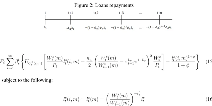
Figure 2: Loans repayments
E0
∞ X
t=o
βt s
(
UCS t(i,m)
"
Ws
t(m)
Pt
ls
t(i, m)−
κw
2
Ws
t(m)
Ws
t−1(m)
−πlw
t−1π1−lw
2 Ws t Pt # − l s
t(i, m)1+φ
1 +φ
)
(15)
subject to the following:
ls
t(i, m) = l s t(m) =
Ws
t(m)
Ws
t−1(m)
−εlt
ls
t (16)
In equilibrium, the labor supply of patient household (s) - and symmetrically for household (m) - is
given by the following:
κw πw
s
t −π lw
t−1π1−lw
πws
t =βsEt
λs t+1 λs t
κw πw
s
t+1−πtlw−1π1−lw
π
wS
t+1
πt+1
!2
+ (1−εI t)l
S t +
εl
t(lts)1+φ
ωs tλst
(17)
whereωs
t represents the real wage for type (s) andπw
s
t is nominal wage inflation.
2.6
Loan and deposit demand
Loan and deposit contracts bought by households and entrepreneurs represent a basket of slightly different
financial products supplied by a branch of j-banks. The elasticity of substitution terms are stochastic,
which are represented byεbH
t > 1(impatient household loans), εbEt > 1(entrepreneurs loans) andεdt <
−1 (patient household deposits), such that bank spreads can move independently of monetary policy.
Demand for real loans (bI
t) of household i is given by the following:
min{bI t(i,j)}
1
Z
0
rbH
t bIt(i, j)dj (18)
subject to the following:
1
Z
0
bI(i, j)
εbHt −1 εbH t dj εbHt εbHt −1
≥bI
where rbH
t =
h R1
0 r
bH t (j)1−ε
bH t dj
i 1
1−εbHt represents the interest rate on household loans. Impatient
households demand for loans at bank j is represented by the Dixit-Stiglitz aggregator:
bI t(j) =
rbH t (j)
rbH t
−εbHt
bI
t (20)
Gerali et al. (2010) originally consider deposits and loans as one-period contracts. Because we are
analyzing multi-period credit constraints for impatient agents based on expected future income, borrowing
contracts for households will be represented as multi-period contracts. In Brazil, non-earmarked loans
have an average maturity of 48 months. Deposits and loans to firms remain one-period contracts. Debt
structure is modeled following Fortali and Lambertini (2013). In each period t, each household i takes on
a new loan,bI
t(i), constrained by its future income. The amortization rate from the second period onwards
is represented byφdǫ(0,1). The law of motion of impatient household (i)’s outstanding debt is given by
the following:
debtt(i) = (1−φd)debtt−1(i) +bIt(i) (21)
Thus, current debt, debtt, is represented by outstanding debt in the beginning of the period, debtt−1,
excluded current amortization6, and new loans. Loan repayments are illustrated by Fig 2.
Because each impatient household takes on a loan during each period t, current debt can be represented
by:
debtt=bIt + (1−φd)bIt−1+ (1−φd)2bIt−2+ (1−φd)3bIt−3+...
debtt=bIt + (1−φd)debtt−1
Entrepreneurs’ demand for loans at bank j is represented by:
bE t (j) =
rbE t (j)
rbE t
−εbEt
bE
t (22)
On the deposit side, the demand for real deposits(dP
t )of patient household i is obtained by
maximiz-ing the followmaximiz-ing:
max{dP t (i,j)}
1
Z
0
rd t(i, j)d
P
t dj (23)
subject to:
1
Z
0
dPt (i, j)
εdt
−1
εdt dj
εdt εd
t−1
≤dP
t (24)
Aggregate demand for deposit at bank j is given by:
dPt (j) =
rd t(j)
rd t
−εdt
dt (25)
wheredtrepresents aggregate deposits of the economy andrtdis the average deposit interest rate.
rd t =
1
Z
0
rd t(j)
1−εd tdj
1 1−εdt
(26)
2.7
Banks
The main contribution of Geraliet al. (2010) is highlighting that the structure of the banking sector is
characterized by imperfect competition at the retail level, which reflects the reality of the Brazilian credit
market. In 2013, the four largest banks hold a concentration of 75% of deposits7.
Banks have market power to set interest rates on deposits and loans in response to shocks. All financial
intermediation is performed exclusively by banks. In other words, banks receive all deposits and supply
loans to impatient households and entrepreneurs. Every bank must meet the following identity:
Bt=Dt+Ktb (27)
Each j bank must use its individual deposits,Dt, and/or its bank capital,Ktb,to finance overall loans,
Bt– these two sources are perfect substitutes for one another. The proportion of deposits and bank capital
is defined based on exogenous capital-to-assets levels (leverage). A bank’s capital is almost fixed in the
short run, and is accumulated over retained earnings. In this framework, bank capital has an important
role in setting the conditions to the credit supply and in the economics cycle. A negative macroeconomic
environment can lead to a drop in bank profit and capital, which may cause credit conditions to deteriorate
as lower loans supplied to private sector credit, which amplifies the original contraction. Each bank j,
jǫ[0,1], consists of three parts: two “retail” branches and one “wholesale” unit. The wholesale unit
is responsible for managing capital group position and retail branches are responsible for (i) supplying
differentiated loans to impatient households and to entrepreneurs and (ii) for receiving differentiated
deposits from patient households.
7
2.7.1 Wholesale branch
The wholesale branch market is in perfect competition and each wholesale’s loans (Bt) must equal
whole-sale’s deposits,Dt,plus bank capital (Ktb). The cost for moving the capital-to-asset ratio ( Kb
t
Bt ) away from
the target level (υb) relies on wholesale unit. Geraliet al. (2010) set the υb parameter at 9%. According
to the Brazilian Central Bank financial stability report8, the Brazilian banking sector’s capital-to-asset
proportion is approximately 10%.
During each period, the wholesale unit accumulates capital as:
πtKtb = (1−δ b)Kb
t−1+jtb−1 (28)
whereδb represents the cost associated with managing bank capital and jb
t−1 is the overall real profit
made by the three branches. The problem of the wholesale unit is to choose the amount of loans and
deposits that maximizes the discounted sum of real cash flows:
max{Bt,Dt}E0
∞ X
t=o
ΛP
0,t =
"
(1 +Rb
t)Bt−Bt+1πt+1+Dt+1πt+1−(1 +Rdt)Dt+
+(Kb
t+1πt+1−Ktb)−
κkb
2
Kb t
Bt −υb
2
Kb t
#
(29)
Subject to the balance sheet, Bt = Dt +Ktb. When Rbt represents the net wholesale loans rate and
Rd
t the net wholesale deposit rates, both are taken as given. Rearranging (27) and including the constraint
twice (for t and for t+1), we can rewrite the objective function as the following:
max{Bt,Dt}R
b
tBt−RbtDt−
κkb
2
Kb t
Bt −υb
2
Ktb (30)
From first-order conditions we have:
Rbt =R d t −κkb
Kb t
Bt
−υb K
b t
Bt
2
(31)
To guarantee a solution, it is assumed that banks have unlimited access to finance at policy rates
rt. Considering the fact that the wholesale market is perfectly competitive, wholesale deposits rates and
interbank market rate are equal:Rd
t =rt. Thus, we have a (29):
Rtb =rt−κkb
Kb t
Bt
−υb K
b t
Bt
2
(32)
Rearranging, the spread between wholesale loans and deposits rates is given by:
Stw ≡R b
t −rt=−κkb
Kb t
Bt
−υb K
b t
Bt
2
(33)
The capital-to-asset ratio is inversely related to the spread between wholesale loan and deposit rates.
Higher leverage increases the spread and profits per unit of capital. However, if leverage exceeds theυb
target, a quadratic cost is paid and reduces profits. The first order condition requires that loan rates are
chosen such that the marginal cost of increasing leverage is equal to the spread.
2.7.2 Retail branch
Retail banks are monopolistic competitors and consist of loan and deposit branches.
2.7.2.1 Loan branch The retail loan branch from each bank j obtains wholesale loans (Bt) at rateRbt from the wholesale unit, differentiates these loans at no cost and then resells them to impatient households
and entrepreneurs, charging different mark-ups. In order to introduce sticky rates, it is assumed that each
retail bank faces a quadratic cost for changing interest rates on loans. Thus, the retail loan unit maximizes
the following:
max{rbH
t (j),rbEt (j)}E0
∞ X
t=o
ΛP
0,t =
"
rbH t (j)b
I
t(j) +r E t (j)b
E
t (j)−R b
tBt− (34)
−κbH
2
rbH t (j)
rbH t−1(j)
−1 2 rbH t b I t − κbE 2 rbE t (j)
rbE t−1(j)
−1 2 rbE t b e t #
subject to loan demand from impatient households and entrepreneurs:
bIt(j) =
rbH t (j)
rbH t
−εbHt
bIt (35)
bE t (j) =
rbE t (j)
rbE t
−εbEt
bE
t (36)
whereBt(j) = bt(j) =bIt+bEt . Assuming a symmetric equilibrium, first order conditions for s={I,E}
1−εbst +ε bs t Rb t rbs t
−κbs
rbs t
rbs t−1
−1 r
bs t
rbs t−1
+ (37)
+βPEt
(
λP t−1
λP t κbs rbs t+1 rbs t
−1 r
bs t+1
rbs t
2 bs t+1
bs t
)
= 0
whereλP
t represents the Lagrange multiplier for the budget constraint for patient households. After
log-linearizing (35) and assumingεbs
t =εbs(for a simplified case), we have the following:
ˆ rbs
t =
κbs
εbs−1 + (1 +β P)κbs
ˆ rbs
t−1+
βPκbs
εbs−1 + (1 +β P)κbs
Etrˆbst+1+
+ ε
bs−1
εbs−1 + (1 +β P)κbs
ˆ Rbt−
ˆ εbs
t
εbs−1 + (1 +β P)κbs
(38)
2.7.2.2 Deposit branch Retail deposit bank j’s unit collects patient household’s deposits,dP t , and
passes them to the wholesale unit, where deposits are remunerated at ratert. The problem of the deposit
unit is to maximize the following:
max{rd t(j)}E0
∞ X
t=o
ΛP
0,t =
"
rt(j)Dt(j)−rdt(j)d P t(j)−
κd
2
rd t(j)
rd t−1(j)
−1
2
rd tdt
#
(39)
subject to household deposit demand:
dpt(j) =
rd t(j)
rd t
−εdt
dpt (40)
whereDt(j) = dPt(j). After imposing a symmetric equilibrium, the first order condition is given by:
−1 +εd t −ε
d t
rt
rd t
−κd
rd t
rd t−1
−1
rd t
rd t−1
+βPEt
(
λP t−1
λP t κd rd t+1 rd t
−1 r
d t+1
rd t
2
dt+1
dt
)
= 0 (41)
assuming εd
t = εd, in a simplified case), the log-linearization version of eq. (39) consists of the
following:
ˆ rd
t =
κd
1 +εd+ (1 +β P)κd
ˆ rd
t−1+
βPκd
1 +εd+ (1 +β P)κd
Etˆrdt+1+
1 +εd
1 +εd+ (1 +β P)κd
ˆ
rt (42)
unit, as represented below:
jb t =r
bH t b
H t +r
bE t b
E −r tdt−
Kb t
Bt −υb
2
Kb
t −Adj B
t (43)
whereAdjB
t represents the adjustment cost of changing interest rates on loans and deposits.
2.8
Monetary policy and market clearing
The Central Bank sets the interest ratertaccording to Taylor’s rule as the following:
(1 +rt) = (1 +r)(1+φR)(1 +rt−1)φR
πt
π
φπ(1−φR) yt
yt−1
φy(1−φR)
εr
t (44)
in whichris the nominal interest rate at stationary level,φRrepresents the weight of inflation deviation
from the targetπ,φy is the weight imputed to output growth andεrt is a white noise shock, withσr as its
standard deviation.
Market clearing in goods markets is given by the following:
yt=ct+qtk[kt−(1−δ)kt−1] +kt−1ψ(ut) +δb
Kb t−1
πt
+Adjt (45)
wherectrepresents aggregate consumption,ktthe aggregate stock of physical capital,Ktb represents
aggregate bank capital and Adjt are all real adjustment costs of price, wage and interest wage. In the
housing market, the aggregate stock is fixed,h, and equilibrium is set by the following:h=hP
t(i)+hIt(i).
3
Estimation
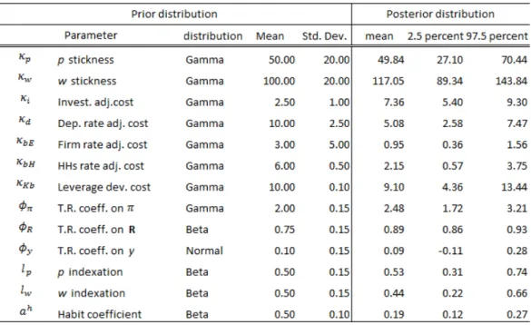
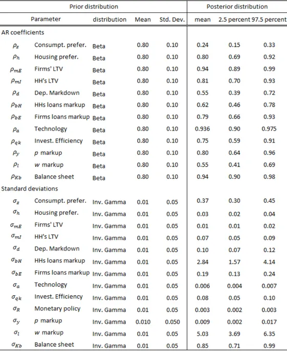
Equations describing the model are used log-linearized around the steady state. We use a Bayesian
ap-proach to estimate the parameters regarding the dynamics (AR coefficients and standard deviations) of
the model, following Smets and Wouters (2003), and calibrate the others. Most credit data used in this
model were discontinued in the fourth quarter of 2012 by the Central Bank of Brazil (from now on, BCB)
and replaced by new data that use a different methodology, beginning as of March 2011. Due to this
circumstance, the sample period was set from 2001:Q1 to 2012:Q4.
3.1
Data and sources
Twelve series are used, as described below. We de-meaned rates, except for monetary policy rates, which
All other variables were detrended, using the HP filter with smoothing parameters set at 1600.
Real consumption: final consumption of households, constant price, seasonally adjusted. Source: IBGE, Contas Nacionais.
Real investments: gross fixed capital formation, constant price, seasonally adjusted. Source: IBGE, Contas Nacionais.
Real housing prices: proxy using civil construction deflator, real estate deflator and rent deflator. Source: IBGE, Contas Nacionais.
Wages: proxy using real payroll and hours per worker, seasonally adjusted. Source: IBGE, BCB
Inflation: quarter over quarter log difference of IPCA. Source: IBGE
Nominal interest rate: SELIC. Source: BCB
Nominal interest rate on loans to households: proxy using non-earmarked loans to households, firms, interest rate on non-earmarked loans to firms and interest rate on non-earmarked loans. Source:
BCB, series 8288, 3959, 3960 and 8287.
Nominal interest rate on loans to firms: rate on non-earmarked loans to firms. Source: BCB, series 8288.
Nominal interest rate on deposits: weighted average interest rate on term deposits, with preset rate, post set rate and floating. Source: BCB, series 32, 33, 40,41,1167,1168,1183 and 1184.
Loans to households: non-earmarked loans to households. Source: BCB, series 3960.
Loans to firms: non-earmarked loans to firms. Source: BCB, series 3959.
Deposits: sum of preset, post set and floating term deposits. Source: BCB, series 33, 41,1168 and 1184.
3.2
Calibrated parameters and Prior distributions
We calibrate 18 parameters, following Castro et al. (2011) and Gerali et al. (2010) for the Brazilian
economy.
For the patient household discount factor, we consider real interest rate ex ante9 during the analyzed
period, such thatβPis set as 0.98. Impatient discount factor (βI) and firms’ (βE) are set to 0.96 because
Geraliet al. (2010) used a 0.2 gap between patient and impatient household discount factor and impatient.
For the inverse of the Frisch elasticity,φ, the share of unconstrained households,µ, and weight of housing
in households’ utility function,εh, we use the same values as in Geraliet al.(2010).
For the capital share of the production function,α, we use 0.448, according to de Castroet al.(2011),
which matches average ration capital GDP for Brazilian economy. With respect to the depreciation rate
of physical capital (δ = 0.015), the markup in goods markets ( εy
εy−1 = 10%) and the markup in labor
markets,( εl
εl−1 = 50%), we also calibrate using de Castroet al.(2011).
Regarding the banking sector, parameters associated with LTV for households are calibrated as
fol-lows: (i) for credit constraints based on future income, we considered LTV, mII = 0.35, to represent
non-earmarked loans to annual disposable income in the Brazilian credit market; (ii) for credit constraints
based on housing, we assumemIH = 0.70, which is the same value as in Geraliet al.(2010). Moreover,
we set entrepreneurs’ LTV,mE, at 0.20, which is lower than the 0.35 LTV used in Geraliet al. (2010).
Non-earmarked loans to entrepreneurs in Brazil are characterized by short term maturity, as BNDES
of-fers long-term loans at rates below market average, which justifies the lower LTV that was seen in the
original paper. Because the average maturity for non-earmarked credit to households is 48 months in
Brazil, we calibrate the amortization rate per period,φd, at 0.0625. For banking capital-to-loan ratio,υb,
we use 10%, according to Brazilian bank system data. Finally, for banking mark ups εbHεbH−1, for
house-holds, and εbEεbE−1, for entrepreneurs, and mark downs,
εd
εd−1, we adjust to reflect the wider spreads seen in
Brazilian data. For the cost of managing the bank’s capital position,δP, the same value from Geraliet al.
(2010) is used.
All prior distributions, means and standard deviations are used as in Geraliet al.(2010).
4
Model Properties
We study how the transmission mechanism of monetary and technology shocks is affected by the
follow-ing two different credit constraints: (i) credit constraints based on household housfollow-ing stock, called the
Benchmark (BK) and (ii) credit constraints based on future income, calledIN.
4.1
Monetary shock
Financial intermediation has an important role in transmitting shocks: in an adverse macroeconomic
environment, banks’ profits decrease and might negatively affect capital – which increases leverage and
may force banks to respond by reducing the amount of loans and thereby may widen the effect of the
original negative shock.
The literature regarding DSGE models with financial friction and financial intermediation shows that,
in an environment with perfect competition, the banking sector amplifies the response to GDP due to a
monetary policy shock – see Christianet al. (2008). Conversely, when considering imperfect competition
in the banking sector, an attenuating effect is found, either with flexible rates, see Andr´es e RacerACE
Table 1: Calibrated Parameters
Figure 3: Impulse response function of a contractionary monetary policy shock
(2010) show that this attenuating effect is mainly due to sticky rates, weakening the transmission from an
increase in interest rate to lending rates. In fact, they illustrate that market power in the banking sector has
limited influence in output - once markups amplify effects for borrowers – although markdown attenuates
changes for lenders.
Here, the traditional interest channel of monetary impulse accompanies the others, see Calza et al.
(2009): (i) nominal debt, i.e., because amortization and interest payments are set in nominal terms, a
fall in inflation rates redistributes resources between lenders and borrowers; (ii) credit constraints, i.e.
innovation regarding monetary policy rates can change loan-to-value ratios because it modifies system
liquidity, impacting borrowers consumption; and (iii) asset-price effects, i.e, monetary policy may affect
housing prices and by doing this affect the value available for borrowing.
In the model with payroll loans, a new channel is added. Shocks in interest rates affect the credit
constraint households because they affect wages, which directly influences their collateral. Thus, families
react by changing their labor supply to reduce this negative effect. Furthermore, the labor supply is
governed not only by traditional substitution and income effects, but also by household decisions aimed
at adjusting the restriction of credit.
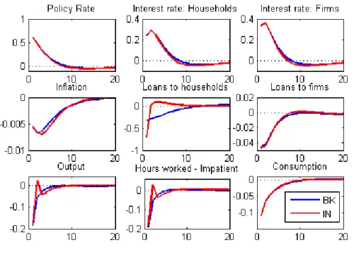
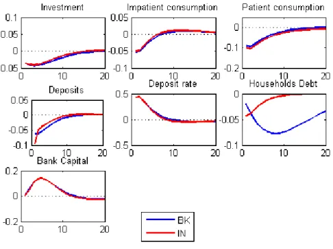
Figures 3 and 4 show impulse responses to an unanticipated 50 basis points exogenous shock in
monetary policy rate,rt. Overall, the direction of responses proceeds as described in the literature.
We can see that transmission to GDP is less persistent in the IN model than in the BK models. As
income falls due to lower wages and lower working demand at first, the impatient agent faces another
Figure 4: Impulse response function of a contractionary monetary policy shock
housing prices, a tightening policy has a larger effect on credit constraints based on income, which leads
agents to experiment with a larger drop in borrowing. To smooth consumption, households adjust their
working hours10 and compensate total gain, so we see a quick recovery in loans to households and also
in debt. However, in the BK model, impatient agents have limited influence in the amount available for
loans because this amount depends on their housing stocks. As housing prices recover slowly, so do loans
to households. In this sense, the behavior predicted by the IN model fits better with the picture presented
by emerging economies, such as Brazil, than that predicted by the BK model, as demonstrated by Fig 1,
which incorporates the stylized facts discussed in the introduction.
4.2
Technology shock
Geraliet al. (2010) show that the presence of a banking system accentuates the endogenous effect of
a technology shock, as impulses exhibit more persistent responses. Furthermore, the banking system
attenuates the response of consumption and output of a technology shock, while the response of
invest-ment is widened. Conversely, banking market power and sticky rates contribute somehow to limiting and
postponing the shock’s transmission, as the responses of borrowing rates are partial and slow.
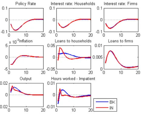
Figures 5 and 6 show responses to a one standard deviation technology shock,aE. Due to a fall in the
prices of final goods, there is a cut in the monetary policy rate, triggering a decrease in lending rates,
mak-ing loans more attractive. Investment is boosted by increases in technology and also by an improvement
10In the modality of payroll loans, banks lend only to families with low risk of becoming unemployed. Therefore, we
Figure 5: Impulse response function of a positive technology shock
in loan conditions. As investment rises, capital prices increase, which increases entrepreneurs’ borrowing
capacity even more .
The household credit borrowing constraint is also affected in two different ways: by improved
col-lateral and by decreased borrowing rates. At first, there is a fall in working hours due to this increase in
productivity. However, as labor becomes more productive, entrepreneurs increase labor demand,
ampli-fying wages and working hours with a lag. In the IN model, collateral is boosted through this channel,
leading to an increase in loans and subsequently in household debt. The BK model also experiences a
loosening in credit constraints as housing prices increase.
The debt deflation channel is worth noting, as in Iacoviello (2005). As the economy experiences
deflation, the expansionary effects of a technology shock are mitigated by the fact that the debt contracts
are set in nominal terms, as a fall in prices induces an increase in debt amount, and this limits the amount
available for borrowing. When considering imperfect competition in the banking sector and sticky rates,
this effect is amplified because the decline in policy rates will slowly and partially repassed to borrowers.
5
Conclusion
This study presented a DSGE model based on Geraliet al.(2010), which is characterized by a
monopolis-tic competitive banking sector and smonopolis-ticky rates, with some adjustments for an emerging market economy.
We explore divergences in the collateral of loans to households. In developed economies, households use
their houses as collateral for loans, but emerging economies, as Brazilian, suffer from lack of collateral,
which leads to unfavorable loan terms and wider spreads. The baseline model was modified by adapting
credit constraints to Impatient households accounting for four years of expected future income and
multi-period loans such that households are allowed to assume debt, which will also affect the amount available
for loans.
We study how this credit constraint behaves when confronting problems based on income changes,
monetary policy and transmission of technology shocks compared with an identical model with credit
constrains based on housing. To do so, we can calibrate and estimate the parameters for the Brazilian
economy using Bayesian techniques. Overall, the direction of impulse responses proceeds as predicted by
the literature in both cases. Notwithstanding the foregoing, the model with households’ credit constraints
based on income responds more quickly to shock than to housing prices, which is the same for the amount
available for loans. In order to smooth consumption, agents compensate lower income and borrowing by
References
[1] Andr´es, J., & Arce, O. (2012). Banking Competition, Housing Prices and Macroeconomic Stability.
The Economic Journal,122(565), 1346-1372.
[2] Arruda, G. (2013). DSGE model with banking sector for emerging economies: estimated using
Bayesian methodology for Brazil.Dissertac¸˜ao, Escola de Economia de S˜ao Paulo,FGV.
[3] Banco Central do Brasil. (2013). Relat´orio de Estabilidade Financeira.v. 12 no2.
[4] Bernanke, B. S., Gertler, M., & Gilchrist, S. (1999). The financial accelerator in a quantitative
business cycle framework.Handbook of macroeconomics, 1,1341-1393.
[5] Carvalho, F., Castro, M., Costa, S., (2013), Traditional and Matter-of-fact Financial Frictions in a
DSGE Model for Brazil: The Role of Macroprudential Instruments and Monetary Policy, Banco
Central do Brasil Working Paper No 336.
[6] Carvalho, C.V., Pasca, N., Souza, L., Zilberman, E. (2014), Macroeconomic Effects of Credit
Deep-ening in Latin America, PUC-Rio Working paper.
[7] Calza, A., Monacelli, T., & Stracca, L. (2013). Housing finance and monetary policy.Journal of the
European Economic Association, 11(s1), 101-122.
[8] Christiano, L. J., Eichenbaum, M., & Evans, C. L. (2005). Nominal rigidities and the dynamic
effects of a shock to monetary policy. Journal of political Economy, 113(1), 1-45.
[9] Christiano, L., Motto, R., & Rostagno, M. (2007). Financial factors in business cycles.Mimeo.
[10] Costa, A.C.; De Mello, J.M.P. (2008) Judicial Risk and Credit Market Performance: Micro
Evi-dence from Brazilian Payroll Loans, InFinancial Markets Volatility and Performance in Emerging
Markets, Sebastian Edwards and Marcio Garcia, editors, Chicago: The University of Chicago Press,
pp. 155-184.
[11] da Silva, M.; Andrade, J.; Silva, G.; Brandi, V. (2012) Financial frictions in the Brazilian banking
system: a DSGE model with Bayesian estimation.Annals of Brazilian Econometric Society Meeting.
[12] de Castro, M. R., Gouvea, S. N., Minella, A., dos Santos, R. C., & Souza-Sobrinho, N. F. (2011).
Samba: Stochastic analytical model with a bayesian approach. Working Paper Series, 239, Banco
[13] C´urdia, V., & Woodford, M. (2010). Credit spreads and monetary policy.Journal of Money, Credit
and Banking, 42(s1), 3-35.
[14] Forlati, C., & Lambertini, L. (2013). Mortgage Amortization and Welfare.Job Market Paper, ´Ecole
Polytechnique F´ed´erale de Lausanne,EPFL
[15] Gerali, A., Neri, S., Sessa, L., & Signoretti, F. M. (2010). Credit and Banking in a DSGE Model of
the Euro Area.Journal of Money, Credit and Banking, 42(s1), 107-141.
[16] Gertler, M., & Kiyotaki, N. (2010). Financial intermediation and credit policy in business cycle
analysis.Handbook of monetary economics, 3(11), 547-599.
[17] Gertler, M., & Karadi, P. (2011). A model of unconventional monetary policy.Journal of Monetary
Economics, 58(1), 17-34.
[18] Goodfriend, M., & McCallum, B. T. (2007). Banking and interest rates in monetary policy analysis:
A quantitative exploration.Journal of Monetary Economics, 54(5), 1480-1507.
[19] Iacoviello, M. (2005). House prices, borrowing constraints, and monetary policy in the business
cycle.American economic review, 739-764.
[20] IMF (2006)Global Financial Stability Report: Market Developments and Issues.
[21] Kornelius, A. (2011). Pol´ıtica monet´aria e compuls´orio em um modelo DSGE com fricc¸˜oes
finan-ceiras.Dissertac¸˜ao, Universidade Cat´olica de Brasilia.
[22] McCulley, P., & Toloui, R. (2008). Chasing the neutral rate down: Financial conditions, monetary
policy, and the taylor rule.Global Central Bank Focus, 2002-2008.
[23] Monacelli, T. (2008). Optimal Monetary Policy with Collateralized Household Debt and Borrowing
Constraints.Asset Prices and Monetary Policy, 103.
[24] Silva, G. C. D. (2013). Avaliando o mecanismo de transmiss˜ao da pol´ıtica monet´aria por meio do
canal do cr´edito: estimac¸˜ao bayesiana em modelos DSGE com fricc¸˜oes financeiras.Tese,
Universi-dade de Bras´ılia
[25] Smets, F., & Wouters, R. (2003). An estimated dynamic stochastic general equilibrium model of the
euro area.Journal of the European economic association, 1(5), 1123-1175.
[26] Taylor, J. B. (1993, December). Discretion versus policy rules in practice.In Carnegie-Rochester
[27] Taylor, J. B. (2008). Monetary Policy and the State of the Economy.Testimony before the Committee
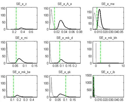
Appendix
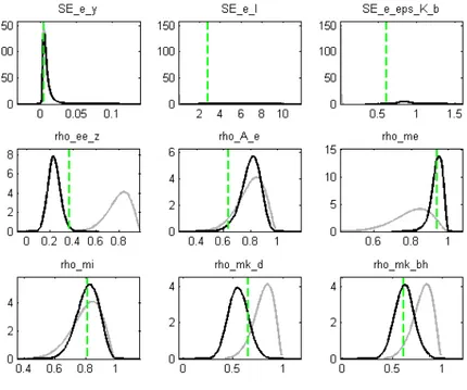
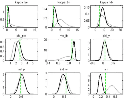
Prior and posterior marginal distribution. The marginal posterior densities are based on 10 chain, each
which 100,000 draws based on the Metropolis algorithm. Black lines denote the posterior distribution
and gray lines the prior distribution.
Figure 8: Prior and posterior marginal distributions