Performance Evaluation of Load Balancing in Hierarchical Architecture
for Grid Computing Service Middleware
Abderezak Touzene1, Sultan Al-Yahai1, Hussien AlMuqbali1, Abdelmadjid Bouabdallah2, Yacine Challal2 1
Department of Computer Science Sultan Qaboos University,
P.O. Box 36, Al-Khod 123, Sultanate of Oman
2
Royallieu Research Center University of Technology Compiegne
P.O. Box 20529, Compiegne, France
Abstract
In this paper, we propose a hierarchical architecture for grid computing service that allows grid users with limited resources to do any kind of computation using grid shared hardware and/or software resources. The term limited resources includes disk or diskless workstations, Palmtops or any mobile devices. The proposed grid computing service takes into account both hardware and software requirements of the user computing task. Our grid system needs to maximize the overall system throughput, minimize the user response time, and allows a good grid resources utilization. On this aspect, we propose an adaptive task allocation and load balancing algorithm to achieve the desired goals. We have developed a simulation model using network simulator NS2 to evaluate the performance of our grid system. We have also conducted some experiments on our test-bed prototype. The performance evaluation measures confirm the good quality (grid saturation level close to 90% of the grid load) of our proposed architecture and load balancing algorithm.
Keywords: Distributed systems, Grid computing, Web-based
applications, Load balancing, Performance evaluation.
1. Introduction
The Computer users, professionals or none professionals, spend their time browsing the Internet or doing any of their daily routine office work (non computing tasks). Many computers are most of the time idle or underutilized. On the other hand there are an increasing number of computing applications that need a huge computing power, which cannot be afforded by a single institution. However, grid computing is a method based on collecting the power of many computers, in order to solve large-scale problems, the parallel processing aspect. On other hand, it offers to independent grid computing services users to share hardware and software grid resources. The grid-computing infrastructure will provide users with almost
unlimited computing power on demand along with a desired quality of service. Grid computing has emerged as an important new field, distinguished from conventional distributed computing by its focus on large-scale resource sharing, innovative applications, and, in some cases, high-performance orientation. Traditional distributed systems can use grid technologies to achieve resource sharing across institutional boundaries. Grid technologies complement rather than compete with existing distributed computing technologies [1]. Grid computing is intended to provide on-demand access to computing, data and services. In the near future grid systems will offer computing services as simply as browsing web pages nowadays [2].
an adaptive load balancing algorithm, which achieve the desired goals.
Our performance evaluation of the load balancing algorithm is based on simulations. Using simulators such as Network Simulator NS2 give us more flexibility to change easily the grid architecture, the power of the processing units, and the network bandwidth of the communication links of the grid system. Changing grid parameter offers to us the ability to test our algorithm under different scenarios, which could not be possible in a real grid with a fixed infrastructure. To measure the performance of our load balancing algorithm we use the saturation level of the grid computed as the ratio of the arrival rate (task/seconds) of total tasks to the grid divided by the total service rate of the grid (tasks/second). The total service rate of the grid is the sum of all the service rate of each workstation in the grid. The saturation level will help us to compare our load balancing algorithm in absolute manner not relative to other approaches. As an example a load balancing which achieves .9 or 90% (at 90% of load the response time is still acceptable) is considered as nearly optimal because whatever algorithm even if it is optimal it will saturate (response time increases exponentially) for load close to 100%.
This paper is organized as follows: Section 2 presents the background and related work. Section 3 presents the layered structure of our grid system. In section 4, we present our analytical model and the load balancing algorithm. In section 5, we present both a simulation model and some experimental results on our test-bed GCS. Section 6 concludes the paper.
2. Backgrounds and Related Works
From the definition of grid computing [3], we can see the following keywords, which summarize grid computing: distributed resources, resource sharing, transparent remote access, infinite storage, and computing power. There are many research problems in the grid. In Condor [4][5], grid computing service is based on cycle-scavenging strategy that uses the idle workstation model. Condor migrate the tasks when the owner of the machine starts using it. In our GCS, task allocation is based on the current load of the workstations participating in the grid. Once a new workstation joins the grid it fixes its share of CPU utilization to be allocated to grid computing service. There is no need to do task migration, grid tasks and workstation owner tasks run using the local CPU scheduler of the workstation. This solution reduces the cost and implementation complexity of task migration mechanism. In Condor there is no load balancing. Tasks distribution is based on a MatchMaker module: Each resource advertises its properties and each task advertises its requirement and then the MatchMaker performs the matching and ranks
them. The resource with the highest rank is selected. In this paper we focus on load balancing and resources management.
Load balancing: is more difficult to achieve in grid systems than in traditional distributed computing environment because of the heterogeneity and the dynamic nature of the grid. Many papers have been published recently to address this problem [6][7][8][9]. Most of the studies present only centralized schemes [10] [11]. On the other hand, some of those proposed algorithms are extensions of load balancing algorithms for traditional distributed systems. All of them suffer from significant deficiencies, such as scalability problems when we talk about the centralized approaches in [11]. A triggering policy based on the endurance of a node reflected by its current queue length is used in [11]. The authors tried to include the communication latency between two nodes during the triggering processes on their model, but lacks including the cost of the actual task transfer. In our model we also consider the node load or saturation level and we do consider the communication task transfer cost. We propose an adaptive load-balancing algorithm, which takes into consideration both computing, and network heterogeneity to deliver a maximum throughput for our grid system. In [12], the authors consider a hierarchical tree structure for grid computing services similar to ours. However, they did not provide any task allocation procedure. Their resource management strategy is based on a periodic collection of resource information by a central entity, which is communication intensive. In our algorithm, resource information collection is done only when it is needed. As an example when a new workstation joins the grid system, it publishes its computing power (CPU speed) on the closest grid manager.
Grid Task Execution Grid Resource Monitoring
Task Allocation & Load balancing
Web Service Task Submission Resource Managements: Different approaches have been
proposed in the literature [18]. Our approach is based on multiple resource manager agents with a hierarchical structure, each one is responsible to track and collect information on its pool of workers in the grid system.
3. Grid Computing Service Architecture
Grid Computing Service (GCS) is a Grid computing service that allows users to submit their computing tasks along with indication of the required hardware or software resources. The GCS system allocates tasks to the available resources and then executes the tasks. After task execution, GCS will reply to the user and send back the results. We identify four main steps in a GCS described in what follows.
3.1 Task Submission Mechanism
The task submission process needs to be as simple as possible and it should be accessible to the maximum number of clients. The best approach for task submission is through web site, using their favorite web browsers. This submission mechanism is also suitable for mobile devices like laptops and mobile phones.
3.2 Task Allocation Mechanism
GCS needs to allocate the computation task to one of the available resources. This may involve task transfer between different components of the GCS system. It may also involve message exchange (such as load balancing information).
3.3 Task Execution Mechanism
After GCS allocates the task to suitable resources, then the task needs to be executed. The resource will perform the required execution (compilation may be needed) and then it will prepare the result file to be sent back to the client.
3.4 Results Return Mechanism
After the execution of the tasks, clients need to be notified whether their tasks have been executed correctly or there were some problems. If the tasks were executed correctly the results will be sent back to the clients. The best approach to display the results is using the Internet browser itself. We propose the following a layered architecture as shown in Figure 1.
Fig. 1 GCS Layered Architecture
3.5 Web Service Task Submission Layer
grid users submit their tasks to the grid system through the GCS web site using their favorite web browser. Our aim is to make access to the grid like browsing internet. The only requirement for the user to access the grid is to have internet access and a web browser. In this layer, we deal with user tasks submission and their requirements (resources and quality of service information).
Our grid system has many access points where users can submit their tasks. To minimize the user’s response time, tasks might be directed to an appropriate grid entry using mirror web site mechanisms. Each grid entry point is called a Grid Agent Manager (GAM). A GAM is responsible of a dynamic pool of workers. The Web information service layer offers to the clients some information about statistics, and some information about the expected response time based on the actual overall load of the grid system. Information about load and availability can grid be collected from the below layer. The Web service layer may decide which GAM to direct the client task based on the grid load and the desired user quality of service.
3.6 Grid Resource Monitoring Layer
workers in a given pool reports to their GAM the status of their resources if any significant change has been noticed since the last report. For example if there is an important change in the CPU utilization or other hardware resources, a change of status is reported to the parent GAM. In our implementation we are using Network Weather Service NWS (for the Unix based resources) [20], and we developed our own tracker tool for the windows-based workstations (Visual-Basic). The parent GAM publishes all information about the resources of its pool at the web service layer. GAMs in the grid system may interact and exchange information to achieve load balancing operations.
3.7 Task Allocation and Load Balancing Layer
In this layer we consider two levels of load balancing, and we propose a load balancing algorithm which works similarly for both levels. The lower level of load balancing consists of the GAM, which distributes the users tasks (load) received from the above layer to the receptor workers of its pool. A worker is declared as a receptor if its CPU utilization is below a given threshold. The load balance strategy is to distribute uniformly the load on the receptor workers. The higher level load balancing is performed at the GAMs level. Whenever a GAM sees that its workers have reached their saturation level (overloaded) and the incoming arrival rate is high, the GAM may decide to direct the over-flow incoming tasks rate to another GAM on the Grid system. In fact the GAMs exchange information about processing availability of their pools. The extra-load at any GAM will be distributed uniformly to other receptor GAMs. A receptor GAM is a GAM with receptor workers. The load balancing algorithm is discussed in more detailed in section 4.
3.8 Grid Task Execution Layer
This layer is the lowest layer and it is mainly responsible to perform tasks execution. It consists also in updating the status of the hardware and software resources at a given computing unit. In this layer, some statistics on the usage of the resources are computed as an example: the average task size, average task execution time are continuously calculated and updated at the GAM levels. Information such as average task execution time is an important parameter in our model, it can be use to determine the computing capacity (number of task per unit of time) at a given computing node and thus the computing availability in a given pool of workers.
Failures can occur in this layer, a worker may fail or simply the owner of the worker machine shuts it down.
Each GAM monitors the tasks that have been sent for execution. It set a timeout parameter for each of them. After passing the timeout, it will resend them to other workers.
4. Load Balancing Algorithm
In this paper we present an adaptive, distributed and sender initiator load balancing algorithm in a grid environment. Our algorithm takes into account the processing capacity of the nodes and the communication cost during the load balancing operation. The class of problem we address is: computation-intensive and totally independent tasks with no communication between them. A task is a user source program written in any programming language. The user program needs to be compiled first then executed.
4.1 Load Balancing Model
Actual Processing Capacity (APC): Actual processing capacity of the system,
L PC APC
Grid Processing Capacity (GPC): the maximum processing capacity (tasks/seconds) at “Grid threshold” utilization. We assume that the CPU is shared between the node owner tasks and the grid tasks. In our model the node owner is the one who decides what will be the share of CPU (percentage) he/she delegates to the GCS. This share is what we call “Grid threshold” utilization.
Available Grid Processing Capacity (AVGPC): The number of tasks/seconds the node can perform until it reaches its maximum allowed grid processing capacity GPC. In other words, the additional load which can be offered for grid computations. AVGPCGPCAPC. All the above parameters are dynamically computed except PC.
Example:PC500t/s, L30%. If the grid threshold is 80%, then: APC 500 0.30 150 t/s,
s t
GPC 500 0.80 400 / , and the available processing capacity: AVGPC 400150250t/s.
4.2 Workers Level Load Balancing
them. This will reduce the number of messages to be exchanged between the manager and its workers. The manager keeps the workers load status on a list.
The tracking of the resources is event driven and not periodical to minimize message exchange between the GAMs and their workers. In the pool, only underutilized workers will report their available processing capacity
AVGPC and only when they notice a significant change in
their values. Those workers will be called receptors. The GAM distributes the received tasks between the receptors according to their reported AVGPC to maximize the throughput of the group. If
N
is the number of received tasks at a given GAM, we define the following parameters:Total Processing Capacity (TPC) of the pool: is the summation of the processing capacities of the pool's
members.
n
i PCi
TPC
1 ().
Total Available Processing Capacity (TAPC) of the pool: is the summation of the available processing capacities of the receptors in the group.
n
r AVGPC r
TAPC
1 ( ).
Receptor Share (sharer(i) ): is the number of tasks to be
given to receptor i: N
TAPC AVGPC Sharer(i) r(i).
Example: If manager GAM1 received 200 tasks and it has three underutilized (receptors) workers r1, r5 and r7 with
AVGPC of 250, 300, and 140 tasks/sec respectively, then:
sec / 690
140 300
250 tasks
TAPC
tasks
Sharer .200 72
690 250 ) 1
(
tasks
Sharer .200 87
690 300 ) 5
(
tasks
Sharer .200 41
690 140 ) 7
(
4.3 GAMs Level Load Balancing
Let us now focus on the GAMs interconnection structure and explain how the interaction between the GAMs of the grid helps to maximize the overall throughput or what we call GAMs level load balancing. We propose to arrange the GAMs of the Grid according to a tree structure to help each others. The tree structure is selected to ensure the scalability (add/remove GAMS) and minimize the communication between the GAMS.
The tree structure is also used to ensure that only one load balance operation at a given GAM can be initiated any time. Having more than one load balance operation at a time may induce information inconsistency and then wrong load balance operations. Exchanging information between the GAMs of the grid uses a token message to be
circulated on the tree. The token message contains the global view of the Grid system. This token message contains the following information about each GAM:
Manager ID: the communication address of the manager.
Total Available Processing Capacity TAPC of the GAM.
Status: the status of the pool, which can be one of the following:
- Neutral (N): Pool under normal load.
- Receiver (R): Available TAPC is high (Pool is under-utilized), ready to receive new tasks and thus increases the throughput.
- Sender (S): Small TAPC and the pool of workers are overloaded. Need to transfer some load to other pools (GAMS) to help.
Example: A sample of the token message could be the following:
From this token message, we can see that GAM M1 is Receiver. The total available processing capacity of the pool is 500 tasks/sec. On the other hand GAM M3 is a Sender. It has an overload of 400 tasks/sec. Some GAMs may receive much more requests than others. When a GAM keeps receiving tasks when its pool of workers is overloaded, the GAM queues up the requests and change its status to sender. A request for help (token information) is generated and transmitted to the parent node in the tree. The parent node rely the token to its parent until it reaches the root GAM. Similarly, an underutilized GAM changes it status to Receiver and then generates a token to be relied to the root GAM passing through the parents path in the tree. At any time the root GAM look at the received tokens and may decide to start a new load balancing operation between tasks. If there is one Sender and more than one Receiver, the root GAM will compute the share of load to be transferred from the Sender GAM to the Receiver GAMS as follows:
Calculating the GAMs share: Since each GAM is connected to another GAM using probably different type of network (different network speed) and each GAM may has a different total available processing capacity TAPC, then when a Sender GAM wants to distribute the extra tasks to the other Receiptor GAM, it needs to take into consideration both factors Receptor TAPC and also link speed from the Sender GAM and the Receptor GAMs. Pools with high processing capacities and fast network connection should get more tasks than pools with low
GAM M1 M2 M3 M4
Status R N S R
processing capacities and slow network connection. We express the network speed or capacity in terms of number of task transferred per second (tasks/sec) [19].
For each Receptor GAM we calculate the load share that it will receive from the Sender GAM depending on its reported APC and its network connection speed (network speed between the sender and the receiver). The load that can be received at a Receptor GAM is the minimum between its reported APC and the network link capacity.
)
_
,
min(
_
offered
TAPC
NW
Capacity
APC
.Then we can define, the Grid Total Available Processing Capacity (GTAPC) as the sum of the APC_offered for all
the Receiptor GAMs:
rec
d(rec) APC_offere
GTAPC .
And then we can calculate the share for each receiver
GAM as: N tasks
GTAPC i offered APC
Sharerec i .
) ( _
)
(
Example: If GAM M1 has N=1000 unprocessed tasks, and the following token information, then it will distribute the load as follows:
M2 can offer up to 700 tasks/sec, but since we can transfer a maximum of 200 tasks/sec over the link connecting M1 and M2, then M2 can only supply 200 tasks/sec.
M3 can offer up to 550 tasks/sec, and since the link can offer that amount then M3 can supply the 550 tasks/sec.
M4 can offer up to 600 tasks/sec, and since the link can offer that amount then M4 can supply
the 600tasks/sec. sec
/ 1350 600 550
200 tasks
GTAPC .
Share tasks
gam .1000 149
1350 200 ) 2
(
Share tasks
gam .1000 407
1350 550 ) 3
(
tasks
Share gam .1000 444
1350 600 ) 4
(
The root node generates and sends a message to the Sender with the calculated shares to be distributed to the Receptor GAMS accordingly. In the case of two or more Sender GAMs, the root will select the most overloaded one will be selected and performs the above load balancing operation. The remaining Sender GAMs will be queued up for the next operation if there are new Receptors. This schema is starvation free because an
unselected Sender will age (will be more and more overloaded then it will have a chance to be selected.
5. Performance Evaluations of our GCS
In this section we present some experimental results conducted on our GCS prototype, which has been implemented using Java RMI system [20]. We also provide a simulation model, which helped us to study the behavior of our GCS under different system parameters: varying the workers CPU speed and varying the network bandwidth between the GAMs.
5.1 GCS Test bed Experimental Results
We have implemented our grid system using Java RMI technology. The choice for Java RMI technology to implement grid computing services is the object of another paper [21]. We just summarize our findings by the fact that all the grid services defined as a standard in [2], either they are supported in Java RMI technology or might be implemented simply. Our prototype Grid system is composed of 8 GAM single-processor Leo Presario Workstations. Each node (GAM) has a single 900 MHZ Pentium III processor with 128 MP RAM and 40 GB IDE Disk. These nodes are connected by an 8-port Myrinet switch. On the other hand, these nodes are connected with Ethernet LAN network to their pool of workers. In our prototype we use 24 workstations (workers) running under RedHat9 Linux operating system, with kernel version 2.4.20-8.
Test Task: During these experiments, we have used a task that performs 25x25 matrix multiplication. The task starts by creating two 25x25 matrices, and then performs the multiplication. Our test task is written using java. Each worker needs to compile and then execute the task. When conducting the grid tasks experiments, workstation owner are executing their tasks simultaneously, which will create a non uniform load in the workstations even if the grid tasks are uniform.
Worker Level’s Load Balancing Evaluation
Our objective in this set of experiments is to measure the quality of our load balancing algorithm GAM worker (worker level). During this set of experiments, we will measure the user response time and the system throughput.
Uniform Load Distribution Experiment: We use one GAM with 12 workers in the pool with no load balancing algorithm.
Load Distribution Experiment: Same configuration as in the previous but with load balancing.
Double the number of Workers Experiment: We use one GAM with 24 workers in the pool. Manager GAM1 GAM2 GAM3 GAM4
Status S R R R
The manager is using the proposed load balancing algorithm to distribute the tasks.
Figure 2, represents the user response time for the different experiments for evaluating the load balancing at worker level. It shows clearly the benefit of having our load balancing algorithm compared to the version without load balancing (NoLB). In other hand, we can also see the good performance of our algorithm when we double the number of workers (1M_24W_LB), the response time is reduced to almost half which is very good.
Response time For worker level load balancing evaluation
4.34 4.88 7.24
13.09
18.43 20.52 29.17
39.9
5.87 7.81
13.18 27.14
36.87 43.55
50.63 80.25
7.07 12.12
18.56 43.82
52.72 70.54
90.93 130.94
0 20 40 60 80 100 120 140
25 50 100 250 300 350 450 550
Input Rate (task/sec)
R
espo
n
se
t
im
e
(
sec)
1M_24W_ LB 1M_12W_ LB 1M_12W_No LB
Fig. 2: Worker level load balancing
GAMs Level’s Load Balancing Evaluation
Unbalanced Load Traffic: In this experiment, we use three GAMs. Each GAM manages a pool of eight workers. In this experiment, the load is directed to only one GAM (unbalanced load traffic).
Balanced Load Traffic: In this experiment we, use three managers. Each GAM manages a pool of 8 workers. In this experiment, we consider different load rates directed (independently) to three GAMs (balanced load traffic).
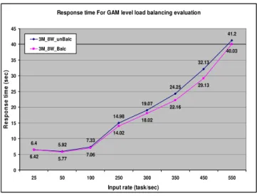
Response time For GAM level load balancing evaluation
6.4 5.92 7.33 14.98
19.07 24.25
32.13 41.2
6.42 5.77 7.06 14.02
18.02 22.16
29.13 40.03
0 5 10 15 20 25 30 35 40 45
25 50 100 250 300 350 450 550 Input rate (task/sec)
R
e
s
pons
e
t
im
e
(
s
e
c
)
3M_8W_unBalc 3M_8W_Balc
Fig. 3: GAMs level load balancing
Figure 3, shows that directing the load independently to three GAMs give better results than directing the load to one GAM only. These results are expected because it will reduce the communication cost due to tasks transfer between GAMs. We can see clearly that after the rate 250 tasks/sec the two curves are separated, it corresponds exactly to the saturation rate for the target GAM. Beyond this saturation rate the GAM starts to direct the overflow rate of tasks to other GAMs and hence the communication cost becomes important. Note that the difference between these two curves is small because communication between GAMs uses the fast full duplex Myrinet switch that provides 2+2 Gigabits/sec.
5.2 Simulation Results Using NS2
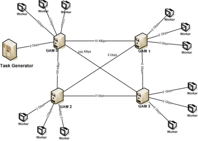
The objective of the simulation is to study the performance of our GCS and the load balancing algorithm under different workers speed and different network bandwidth between GAMs. We carried out simulations using network simulator NS2. We considered a topology with 3 GAMs, where each GAM manages a pool of 8 workers. Figure 4 illustrates this topology.
Fig. 4: NS2 scenario
We assumed that tasks submission to our Grid Computing Service follows a Poisson law with parameter Ȝ, which corresponds, to the arrival rate of the tasks to the system. We supposed also that the number of instructions in a task, and hence the task’s execution duration follows an exponential distribution with parameter ȝ, which corresponds to the average execution duration of a task. Impact of the input rate:
In a first stage, we were interested in evaluating the impact of the input rate (tasks per second) on the performance of GCS. We considered two cases: in a first case we submitted the tasks to the same GAM (unbalanced arrival of tasks into the system). In the second case, we distributed the arrival of the tasks uniformly over the three GAMs of the system. Figure 5 illustrates the response time of the system with respect to the input rate. We notice that the system behaves better when the tasks arrival is uniform (same arrival rate) over the three GAMs. Indeed, this minimizes the communication delays due to load balancing at the GAM level.
Fig.5: Average response time of GCS with respect to input rate.
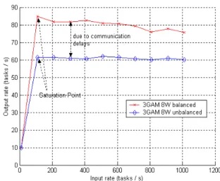
Figure 6, illustrates the output rate of the system with respect to the input rate. We notice again the difference in output rates due to communication delays between GAMs. We remark that at 110 tasks/s the system reaches the saturation point and its output rate becomes constant.
Fig. 6: Output rate (tasks/s) with respect to input rate.
Impact of the GAMs’ links bandwidth:
In a second stage, we were interested in evaluating the impact of the bandwidth between GAMs. Figure 7 illustrates the average response time with respect to the available bandwidth between GAMs. We notice that, when the available bandwidth between GAMs exceeds 1.5Gbps, the communication delays between GAMs become negligible this is in total agreement with our experimental measures.
Fig. 7: Response time with respect to bandwidth between GAMs
Impact of the different load generation methods for GAMs ( not including the communication cost):
In the following experiments we did not consider the communication cost. We run the experiments with different load generation methods. The grid load is defined as
GPC
Uniform generation Method: the total grid load is distributed evenly to all GAMs of the grid (
Ms NumberofGA
GAM
). The experiment is
designed to assess the workers level load balancing.
This method will help us to assess how good the GAM level load balancing algorithm is.
Maximum available load: All the grid tasks will be directed to the GAM with maximum available processing capacity (less loaded). This method will help us to compare with previous method.
Experimental Results:
Table 1 shows the simulation results for different grid load. The uniform generation method gives a low response time up to grid load 90%.
Table 1: Average response time result (seconds)
Methods 10% 50% 70% 90%
Uniform generatio
n Method 0.27 0.38 0.42 0.53
Minimum Available
load 1.55 1.68
Maximum Available
load 0.004 0.078 0.32 0.38
The minimum available load method shows bad results. Indeed most of the tasks are transferred to the overloaded GAM. This GAM is continuously asking for help from the over GAM (GAM level load balancing) but meanwhile (time to perform a load balancing operation), a lot of new tasks may arrive (single entry point of tasks), which saturates the grid system very early (50% grid load).
The Maximum available capacity method shows very good response time. In this case most of the tasks are executed within its pool of workers. Extra load will be distributed among the other GAMs
Impact of the communication cost:
In this experiment, we take into account the network cost in the decision of the load balancing algorithm. The experiment consists of four GAMs with three workers. The initial available load capacity of each worker is 50 tasks per seconds. See figure 8.
Fig. 8: Topology of the Experiment
Table 2 shows that when we include the communication cost in the decision of the load balancing algorithm gives acceptable results up to 60% of the grid load. The second column of table 2 shows the response time when the communication cost is included in the topology but not included in the decision of the load balancing algorithm. In this case the grid saturates at grid load around 30%. This experiment show that our algorithm which takes into account the communication cost is giving good results including the communication overhead.
Table 2: Average response time (seconds)
LOAD With
Communication
Without
Communication
10% 0.33 0.33
20% 0.076 0.076
30% 0.25 2.307
40% 0.265
50% 0.266
60% 0.473
5. Conclusion
tends to minimize the overall tasks response time and maximize the grid system throughput (saturation level close to 100%). Simulation results shows that our load balancing algorithm (without communications) has a saturation level (90%) close to the optimum. When we take into consideration the network links bandwidth our load balancing performs well up to 60% of the grid load in our example of relatively slow networks. In our current version of the grid-prototype we did not implement yet fault tolerance and any security issues. In the future work we will investigate the fault tolerance, security aspects and analytical models to measure performance of our grid computing service.
References
[1] I. Foster, C. Kesselman, S. Tuecke. The Anatomy of the Grid: Enabling Scalable Virtual Organizations. International J. Supercomputer Applications, 15(3), 2001.
[2] T. DeFanti and R. S. Teleimmersion. The Grid: blueprint for a New Computing Infrastructure, In Foster, I. and Kesselman, C.eds. Morgan Kaufmann, 1999, 131-155.
[3] Douglas Thain, Todd Tannenbaum, and Miron
Livny, "Condor and the Grid", in Fran Berman, Anthony J.G. Hey, Geoffrey Fox, editors, Grid Computing: Making The Global Infrastructure a Reality, John Wiley, 2003. ISBN: 0-470-85319-0 [4] Jim Basney and Miron Livny, Managing Network
Resources in Condor, Proceedings of the Ninth IEEE Symposium on High Performance Distributed Computing (HPDC9), Pittsburgh, Pennsylvania, August 2000, pp 298-299 .
[5] H.A.James and K.A.Hawick. Scheduling Independent Tasks on Metacomputing Systems. Proc. ISCA 12th Int. Conf. on Parallel and Distributed Computing Systems (PDCS-99). Fort Lauderdale, USA, March 1999.
[6] T.L. Casavant and J.G. Khul. A taxonomy of scheduling in general purpose distributed computing systems. IEEE Transaction on Software Engineering, Vol. 14, No. 2, 1999, pp.141-153.
[7] C.Z. Xu and F.C.M. Lau. Load Balancing in Parallel Computers: Theory and practice. Kluwer, Boston, MA, 1997.
[8] M.J. Zaki, W. Li , and S. Parthasarathy. Customized dynamic load balancing for network of workstations. In Proc. of the 5th IEEE Int. Symp. HDPC, 1996, pp. 282-291
[9] V. Subramani, R. Kettimuthu, S. Srinivasan and P.Sadayappan, Distributed Job Scheduling on Computational Grid Using Multiple Simultaneous Requests. Proc. of 11-th IEEE Symposium on High
Performance Distributed Computing (HPDC 2002), July. 2002.
[10] M. Arora, S.K.Das and R. Biswas. A De-Centralized Scheduling and Load Balancing Algorithm for Heterogeneous Grid Environments. ICPP Workshops 2002: 499-505.
[11] B. Yagoubi and Y. Slimani. Dynamic Load
Balancing Strategy for Grid Computing. Transactions on Engineering, Computing and
Technology. Vol 13, 2006, pp. 260-265.
[12] Bo Hong and Viktor K. Prasanna, Adaptive
Allocation of Independent Tasks to Maximize Throughput, IEEE Transactions on Parallel and Distributed Systems, Vol. 18, No. 10, 2007, pp. 1420-1435.
[13] L. Marchal , Y. Yang, H. Casanova, and Y. Robert. A Realistic Network /Application Model for Scheduling Divisible Loads on Large-scale Platforms, 19th IEEE International Parallel and Distributed Processing Symposium (IPDPS05), 2005.
[14] O. Beaumont, A. Legrand, Y. Robert, L. Carter, and J. Ferrante, Bandwidth-centric Allocation of Independent Tasks on Heterogeneous Platforms, 16th IEEE International Parallel and Distributed Processing Symposium (IPDPS02), 2002.
[15] O. Beaumont, A. Legrand, Y. Robert, L. Carter, and J. Ferrante, Bandwidth-centric Allocation of Independent Tasks on Heterogeneous Platforms, 16th IEEE International Parallel and Distributed Processing Symposium (IPDPS02), 2002.
[16] C. Banino, A Distributed Procedure for Bandwidth-Centric Scheduling of Independent-Task Applications, 19th IEEE International Parallel and Distributed Processing Symposium (IPDPS05), 2005.
[17] T.K. Apostolopoulose, G. C.Oikonomou. A scalable, Extensible framework for grid management. IASTED International Conference Feb. 2004, Austria.
[18] G. Shao, F. Berman, R. Wolski. Master/Slave Computing on the Grid. In Proceedings of the 9th Heterogeneous Computing Workshop, (Cancun, Mexico, 2000), 3-16.
[19] R. Wolski. Experiences with Predicting Resource Performance On-line in Computational Grid Settings. ACM SIGMETRICS Performance Evaluation Review, Volume 30, Number 4, pp 41-49, March, 2003.