www.ann-geophys.net/27/2881/2009/
© Author(s) 2009. This work is distributed under the Creative Commons Attribution 3.0 License.
Annales
Geophysicae
Simultaneous imaging of aurora on small scale in OI (777.4 nm) and
N
2
1P to estimate energy and flux of precipitation
B. S. Lanchester1, M. Ashrafi1, and N. Ivchenko2
1School of Physics and Astronomy, University of Southampton, UK
2Space and Plasma Physics, School of Electrical Engineering, KTH, Stockholm, Sweden
Received: 19 February 2009 – Revised: 22 June 2009 – Accepted: 13 July 2009 – Published: 22 July 2009
Abstract. Simultaneous images of the aurora in three emis-sions, N21P (673.0 nm), OII (732.0 nm) and OI (777.4 nm),
have been analysed; the ratio of atomic oxygen to molecular nitrogen has been used to provide estimates of the changes in energy and flux of precipitation within scale sizes of 100 m, and with temporal resolution of 32 frames per second. The choice of filters for the imagers is discussed, with particular emphasis on the choice of the atomic oxygen line at 777.4 nm as one of the three emissions measured. The optical mea-surements have been combined with radar meamea-surements and compared with the results of an auroral model, hence show-ing that the ratio of emission rates OI/N2can be used to
es-timate the energy within the smallest auroral structures. In the event chosen, measurements were made from mainland Norway, near Tromsø, (69.6 N, 19.2 E). The peak energies of precipitation were between 1–15 keV. In a narrow curling arc, it was found that the arc filaments resulted from energies in excess of 10 keV and fluxes of approximately 7 mW/m2. These filaments of the order of 100 m in width were em-bedded in a region of lower energies (about 5–10 keV) and fluxes of about 3 mW/m2. The modelling results show that the method promises to be most powerful for detecting low energy precipitation, more prevalent at the higher latitudes of Svalbard where the multispectral imager, known as ASK, is now installed.
Keywords. Ionosphere (Auroral ionosphere; Particle pre-cipitation; Instruments and techniques)
1 Introduction
The highest spatial and temporal resolution images of au-rora show that there is a large variety of auau-roral fine-scale
Correspondence to:B. S. Lanchester ([email protected])
structure (tens of metres across the magnetic field) which is highly dynamic. Processes operating on small scales often affect the bulk properties of the plasma, and so characteris-ing and understandcharacteris-ing the structurcharacteris-ing is important. In au-rora, this structuring can be directly observed in the distribu-tion of emitted light. Accelerated electrons colliding with atmospheric constituents excite a range of emissions, pri-marily determined by the heights at which the electrons are stopped. Low energy electrons give rise to atomic oxygen emissions at heights of 200–500 km, while high energy elec-trons reach down to approximately 100 km and give a spec-trum dominated by molecular emissions. Advances in optical detectors and computer performance allow optical imaging of the aurora at unprecedented spatial and temporal resolu-tion. The advent of the Electron Multiplying Charge Cou-pled Devices (EMCCD) has effectively eliminated the prob-lem of read-out noise, and made possible low-light imaging at high frame rates. The increased sensitivity allows imaging in narrow spectral regions, isolating emissions resulting from electrons of different energies. The combination of a number of imagers operating in different spectral lines allows time-dependent, two-dimensional energy spectrum maps of the auroral precipitation to be generated. This is the best avail-able “image” of the acceleration processes. In situ spacecraft provide more accurate information on particle distribution functions, electric fields and plasma densities than remote sensing, but they lack the detailed two-dimensional structure and rapid evolution of optical measurements.
incorporated into the model comparisons. The first aim of the work is to validate the model, using measured emission rates, which require a full understanding of the cross sections involved. Following from this is the further aim of finding a theoretical basis for the energy input into the variable and dynamic auroral structures observed.
Semeter et al. (2001) used multispectral imaging of dis-crete arcs in four different wavelengths, with particular at-tention to two spectral bands centred on 427.8 nm (N+2) and 732.5 nm (O+). The work was concentrated on low energy
(<1 keV) precipitation in discrete aurora, making use of the ratio of the two emissions within small scale structure in the zenith. They found that the low energy emissions from O+
can be strong even within narrow structures during arc for-mation. The spatial resolution was 300 m at 100 km altitude, and time resolution of 0.3 s. The present work provides even higher resolution, and uses different and more suitable opti-cal emissions as input, in particular the atomic oxygen line at 777.4 nm. Gustavsson et al. (2000) have also used atomic oxygen emission at 844.6 nm for spectral analysis of a fold-ing arc. They combined this emission with 427.8 nm (N+2) to obtain characteristic energies and fluxes. Their data are from the Auroral Large Imaging System (ALIS) chain of cameras, with a wide field of view.
The instrument known as ASK (for Auroral Structure and Kinetics), images a region of only 3◦×3◦ in the magnetic
zenith, which gives a spatial resolution of 10 m at 100 km height and a sampling time as low as 20 ms. The combina-tion with simultaneous images from more than one spectral bandwidth provides the information about the changes in en-ergy distributions at these scales. The first results from the ASK instrument used the ratio of O+2/O emission rates to study changes in both the energy distributions and the fluxes across narrow filaments (Dahlgren et al., 2008b). The present work uses emissions from N21P bands and atomic oxygen
to investigate variations in energy and flux during an interval of a few minutes of auroral activity.
The auroral model used in this work is a time-dependent model which solves the electron transport equation, the cou-pled continuity equations for all important positive ions and minor neutral species, and the electron and ion energy equa-tions. The multistream solution of the electron transport equation has updated cross sections and energy grid from Lummerzheim and Lilensten (1994). The ion chemistry part of the model developed by the Southampton group (Palmer, 1995) is described in detail in the appendix of Lanchester et al. (2001). Timesteps are chosen to match the auroral ob-servations and conditions, usually at sub-second resolution for active aurora. The main input required is an estimate of the shape and peak energy of the electron energy spectrum at each time step, and the magnitude of the precipitation en-ergy flux (Lanchester et al., 1997). Other inputs to the model calculations are electron impact cross sections of the major atmospheric neutral constituents. Cross sections for excita-tion and the energy losses of each individual excited state are
required to calculate the energy degradation at each step, and the resulting emission profiles.
2 Instrumentation
The ASK instrument is made up of three cameras (ASK1, ASK2 and ASK3), each equipped with an Andor iXon EM-CCD detector with 512×512 pixel chip. The optics
in-cludes a Kowa 75 mm F/1 lens, which gives a field of view of 6◦×6◦. However, each camera is fitted with a removable
2×telescope to make a 150 mm, f/1.0 lens. This gives the
field of view of 3◦×3◦ which is equivalent to 5×5 km at
100 km height. The time resolution used here is 32 fps. The instrument is pointed toward magnetic zenith. Selected nar-row passband filters are fitted to each camera. The data are background subtracted and calibrated using star fluxes. Mea-sured intensities of the stars are compared with theoretical tabulated values. The rationale for the choice of filters used in the three cameras is discussed in Sect. 3. The ASK instru-ment also has two photometers in its assembly which were not used in the present work.
Height profiles of electron density in the ionosphere are obtained with the EISCAT radar situated near Tromsø, Nor-way (69.6 N, 19.2 E). The present observations were made with the UHF antenna, pointed along the local magnetic field line. The field of view has half width of 0.6◦. The radar ex-periment “arc1” was designed to study the auroral ionosphere using 128 different 64 bit codes to give high time resolution (0.44 s) and a good range resolution (0.9 km) without range side lobes, between 96 km and 422 km. The resulting power spectra are fitted to give electron and ion temperatures and electron densities.
3 Spectral bands and lines measured with ASK
The following sections describe the motivation for the filters used in the three ASK cameras in the present work. In par-ticular the choice of filter for ASK3 is provided in greater detail, since the atomic oxygen emission is crucial for mea-suring the low energy component in the study of energy dis-tributions using multispectral imaging.
3.1 ASK1: N21P bands
In the present work the ASK1 filter was centred on 673.0 nm, with width of 14 nm. This filter transmits two N21P
vibra-tional band emissions from transitions (4,1) and (5,2) of the B35gstate to the A36u+state. In modelling the emissions,
the choice of cross section is important. For the N21P
0 200 50
100 150 200 250 300 350 400 450 500
Height (km)
N 2 − 6730
0 50
O+ − 7320
0 50 100
OI − 7774
0 20 40
OI−D − 7774
0.02 0.04 0.07 0.1 0.2 0.4 0.7 1 2 4 7 10 20
keV
Volume emission rates (phot/s/m3)
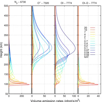
Fig. 1. Modelled height profiles of emission rates using monoen-ergetic input spectra of varying peak energies, and constant flux of 1 mW/m2: (a)N2 1P bands (ASK1),(b)O+line at 732.0 nm (ASK2)(c)777.4 nm from direct excitation (ASK3),(d)777.4 nm from dissociative excitation (ASK3).
calculated with the transport model for a constant input flux of 1 mW/m2 and monoenergetic spectra with varying peak energies. The brightness of emissions from molecular nitro-gen is proportional to the total energy flux. The peak in the emission rate at around 100–110 km results from energies of 10 keV or more.
3.2 ASK2: O+forbidden emission at 732.0 nm
The ASK2 filter is designed to measure emission from the oxygen ion at 732.0 nm, caused by the forbidden O+(2P–2D) transition. The ASK2 filter has a FWHM of 1.0 nm which en-compasses one line of the doublet at 732.0 nm and 733.0 nm. However, the data are contaminated in this wavelength inter-val by the N2 1PG band, and by OH airglow. A full
anal-ysis of the method used to reduce this contamination, and to validify the method to remove the contamination using N2emissions is described in Dahlgren et al. (2008a). The
emission from ASK2 is the result of low energy precipita-tion, with peak emission rates from particles with energies of around 200 eV occurring at heights of 300 km, as can be seen in the second panel of Fig. 1. The figure shows modelled volume emission rates for a steady state solution for different energies, with the same input energy flux of 1 mW/m2.
The metastable O+2P state has a radiative lifetime of ap-proximately 5 s, allowing the possibility of direct observa-tion of plasma drifts in the topside ionosphere. With the
1356 990
1304 8446
7990
7774
P
3
S
3 3D 5S 5P
3s
3s 3p 3p
3s´
2s22p4
Fig. 2. Energy diagram of the lowest triplet and quintet states of atomic oxygen, showing the important transitions (labelled in ˚A).
multispectral imaging of the ASK instrument, the direct im-pact emission can be measured with one camera, while the emission from oxygen ions can be detected in another cam-era after the precipitation creating them has ceased (Dahlgren et al., 2009).
3.3 ASK3: OI emission at 777.4 nm
In choosing the emission for ASK3, several considerations were explored. Low energy electron precipitation is best characterised by an atomic oxygen emission. In addition, in order to quantify the production of the metastable O+2P ions measured by ASK2, a bright emission originating from the same parent species (atomic oxygen) is needed. For ob-servations of highly dynamic aurora with sub-second resolu-tion, prompt emissions are needed, which means that the red (630.0 nm) and green (557.7 nm) oxygen lines are not suit-able. Also, because of the low excitation threshold, a number of mechanisms can produce the O1D and O1S states chemi-cally. Allowed transitions of both neutral and ionized oxygen lie in the UV, so for observations in visible light only transi-tions between the higher-lying states are suitable. Visible emissions from O+lie mostly in the blue region, where they are blended with N+2 1N bands (Ivchenko et al., 2004). Be-sides being weak, the emissions have rather high excitation thresholds (in excess of 40 eV), which makes their excitation quite different from that of the O+2P ions. The most promi-nent atomic oxygen lines are the 3s5S – 3p5P at 777.4 nm
and 3s 3S – 3p 3P at 844.6 nm (see Fig. 2). Both
multi-plets are well known in the auroral spectrum (Christensen et al., 1978). They have excitation thresholds above 10 eV, and therefore are most suitable for characterising low energy precipitation.
10 20 30 40 50 0
1 2 3 4 5 6 7 8 9 10
Energy, eV
Cross section, 10
−18
cm
2
101 102 103 104
10−2 10−1 100 101
Energy, eV
Cross section, 10
−18
cm
2
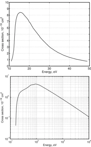
Fig. 3. Emission cross-sections of the 777.4 nm muliplet: top – electron impact on atomic oxygen (derived from Julienne and Davis, 1976), bottom – dissociative excitation of O2(Erdman and Zipf, 1987).
electron impact on atomic oxygen, O+e−→O(3p). The
dis-sociative excitation channel will make the emissions sen-sitive to higher energy precipitation as well as low ener-gies. High spectral resolution observations of the multiplets (Hecht et al., 1985) revealed the broadened component in the 777.4 nm emissions, corresponding to dissociative exci-tation. The 844.6 nm multiplet is less sensitive to dissocia-tive excitation. The second complication is that the 844.6 nm multiplet is fed by cascade from the 3s′ 3D state through
799.0 nm emission. The 3s′ 3D state is excited in the
res-onant transition at 99.0 nm, so that the contribution of the excitation to the 844.6 nm multiplet depends on whether the medium is optically thick or optically thin in the resonant line (Julienne and Davis, 1976). For the optically thick case, cas-cading exceeds direct excitation, and a ratio of about 4 was predicted, while the observed ratios are typically between 1 and 2 (Christensen et al., 1978). Since the transition between the ground state O+3P and the quintet states feeding the cas-cades to the 777.4 nm multiplet are forbidden, reabsorption and radiation trapping is not an issue for that emission. Even though the 844.6 nm is more intense, and apparently less
af-fected by dissociative excitation, the complication of the ra-diation trapping effects and decrease of the detector sensitiv-ity for the longer wavelength together weighed against imag-ing in this line. The 777.4 nm multiplet is used for imagimag-ing with ASK. The ASK3 filter is centred on 777.4 nm with a FWHM of 1.5 nm.
To our knowledge, there is no recent direct measurement of the emission cross-section for the 777.4 nm multiplet. Juli-enne and Davis (1976) present a comprehensive discussion of the cascading processes, noting that cascading contributes about 75% of the emission cross-section for the 135.6 nm line. Over 98% of the cascading proceeds through the 3s–3p emission at 777.4 nm. However, only about 30% is from di-rect excitation to the 3p state, with the rest being the result of cascading from yet higher states. Laboratory measurements presented by Julienne and Davis (1976) concern the emission cross-section of the 135.6 nm line. The absolute calibration of the measurements has been revised by Zipf and Erdman (1985). More recent laboratory measurements by Gulcicek et al. (1988) are of the cross-section of the direct transition to the 3p5P state, i.e. they do not include cascading from the higher lying states. We assume the emission cross-section at the level of 75% of the modelled total emission cross-section for 135.6 nm as given in Julienne and Davis (1976). As shown in the top panel of Fig. 3 the notable feature of the emission cross-section (in agreement with newer measure-ments) is that it is strongly peaked just above the threshold, and decreases rapidly for higher energies. This is natural for spin-forbidden transitions.
The cross-section for dissociative excitation of the 777.4 nm multiplet from O2has been studied, together with
other emissions, by Schulman et al. (1985). The peak emission cross-section value was 4.3×10⁻¹⁸m2, observed
slightly below 100 eV. The emission cross-section was later re-measured by Erdman and Zipf (1987), producing excel-lent agreement around the peak, but slightly different values above the peak. We assume their results for use in the model. The energy dependence is plotted in the lower panel of Fig. 3. The third and fourth panels of Fig. 1 show the volume emission rates for 777.4 nm resulting from both excitation processes as a function of altitude and energy for the same total energy flow of 1 mW/m2. The direct excitation channel exhibits a similar behaviour to the 732.0 nm emission, apart from the lowest energies, where the 777.4 nm is more easily excited. This difference has to do with the lower threshold of the neutral excitation compared to the ionisation-excitation. The dissociative process has lower production rates, except for energies reaching 10 keV.
4 Results
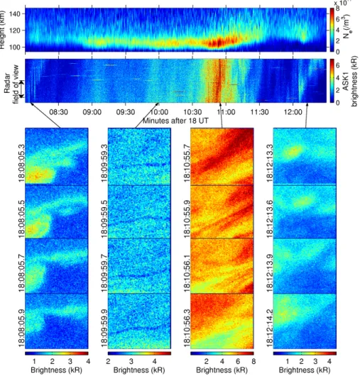
Fig. 4. Overview of the variations between 18:08:00 UT and 18:12:30 UT. (top panel) electron density (second panel) emissions in ASK1 and (lower panels) selected images during 1 s intervals as marked with arrows.
During this time there were several distinct changes in the nature of the observed aurora. Figure 4 is an overview of the radar and optical data for the interval 18:08:00 UT– 18:12:30 UT. The top panel is the measured electron den-sity in the E region from the field-aligned position, between 95 km and 150 km. The second panel is a time series of slices taken across the images from ASK1 (N21P), which were the
brightest of the images from the three cameras during the observations. The slices are made from a central meridian cut, i.e. 3◦ north-south aligned. The approximate position and size of the radar field-of-view is marked on the left-hand axis. Below this panel are sample ASK1 images from four selected intervals, using false colour to demonstrate the small scale variations more clearly. In each interval there is a time sequence lasting less than one second. The first selected in-terval (18:08:05 UT) shows the passage of a curling thin arc across the field of view. A thin arc is in the field of view for about 15 s during which time 5 separate curls (or folds) move across from right to left, folding and unfolding in the
pro-cess. The second interval (18:09:59 UT) shows a period of diffuse aurora with very narrow (<150 m) dark lanes moving through the field of view. The third interval (18:10:55 UT) is at the peak of the brightest event, when the camera mea-sured swirling, narrow filaments. Note that the width of the bright filaments is similar to that of the dark lanes in the previous interval. The final interval (18:12:13 UT) follows a time of lower activity, when more diffuse curl-like patches move across the field of view. Between the third and fourth intervals at 18:11:00 UT–18:11:30 UT, the auroral signature changed from bright and active structures to pulsating and flickering aurora. These changes are not possible to show in still images.
4.1 Flux and energy
10:30 11:00 11:30 12:00 0
5 10 15 20 25 30
minutes after 18 UT
energy flux (mW/m
2)
optical flux radar flux combined flux
10:30 11:00 11:30 12:00
10−1
100
101
102
minutes after 18 UT
peak energy (keV)
mono maxw
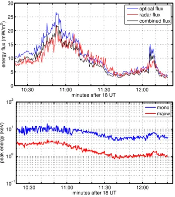
Fig. 5. (a)Total energy flux determined from radar and optical methods.(b)Peak energies of monoenergetic and maxwellian dis-tributions used as input energy spectra for modelling.
the model. That having been achieved, the ratio of emissions within the ASK field of view can be used to give estimates of energies at unprecedented resolution in time and space.
The first input requirement for the model is a time vary-ing set of energy spectra for the precipitatvary-ing electrons at the top of the atmosphere. The method used to obtain such a data set has been described in Lanchester et al. (1998). Ion-isation rate profiles are inferred from radar electron density height profiles, and these are fitted to model ionisation rate profiles generated from both maxwellian and gaussian (10% width) spectra, using a constant downward energy flux and varying peak energies, and with suitable neutral atmospheric profiles for the position and date of the observations. These are obtained from the MSIS-90 thermospheric model (Hedin, 1991). This “flux-first” method is only the first step to find-ing the energy spectra, since the real spectra are not a sfind-ingle well-defined shape, but a mixture of many shapes. The final spectra, both flux and shape, are determined by an iterative process. In the present work we have obtained reasonable fits using a combination of a monoenergetic spectrum (i.e. 10% gaussian) and a smaller contribution to the energy flux from a maxwellian spectrum.
The estimation of energy flux using the “flux-first” method depends on the assumption of a constant recombination rate coefficient. Therefore it provides limits to the magnitude of the energy flux, which may vary as the height of the peak of
auroral precipitation varies. Consequently another method for estimating the flux has been applied for comparison. The surface brightness of nitrogen band emissions can be used as a proxy for flux, since it can be assumed that the emis-sion rate from nitrogen molecules is proportional to the total energy flux. Therefore the integrated brightness of the N2
1P bands in the region of the zenith from the ASK1 cam-era can be converted to energy flux. The ASK1 brightness has been integrated over the same time interval as the radar measurements (0.44 s) and over a field of view correspond-ing to the width of the radar beam. The conversion factor has been taken from Vallance-Jones (1974). This assump-tion will place limits on the flux estimate which may change with the nature of the aurora. The conversion factor applied is 0.36 kR≡1 mW/m2. In addition, the transmission factor through the ASK1 filter has a value of 0.72; this was de-termined using synthetic spectra and the filter transmission curve and is described in more detail in Ashrafi et al. (2009). An interval of two minutes between 18:10:15 UT and 18:12:15 UT has been selected for analysis, corresponding to the time of maximum auroral brightness and electron den-sities shown in Fig. 4, hence providing good E region pro-files for the fitting process. The values of energy flux are shown in Fig. 5a. The red curve is the flux derived from the radar profiles, and the blue curve is flux derived from ASK1 brightness. The latter slightly exceeds the former at times of the most intense aurora, but at other times the two curves are in very close agreement. Both estimates of total energy flux were used as input to the model, and the resulting height profiles of electron density compared with those measured by the radar. After 18:11:00 UT both fluxes were found to be in excess of what is needed to match modelled to mea-sured electron densities. Therefore the flux was reduced at this time by normalising the ASK1 flux to the maximum of the radar flux; the resulting flux is shown by the black curve in Fig. 5a.
The electron density profiles are most useful in determin-ing the peak energy at each time step. As already mentioned, the input spectra are not usually a single shape. For the in-terval chosen, a good fit to the electron density profiles was found from a monoenergetic shaped spectrum, with a “back-ground” maxwellian contribution of 20% of the energy flux. Figure 5b contains the values of peak energy used for each of the contributing distributions. The monoenergetic energies have been fine-tuned by an iterative process, by comparing the profiles of total ionisation resulting from each model run with the electron density profiles at each time step. The time dependent nature of the model means that the final spectral shapes used in the model are quite different from the single monoenergetic or maxwellian used in the flux-first method.
100
120 140 160
height (km) 2
4 6 x 10¹¹
10:30 11:00 11:30 12:00
100 120 140 160
minutes after 18 UT
height (km)
Ne (/m3) 2 4 6 x 10¹¹
Fig. 6. Modelled (top) and measured (bottom) height profiles of electron density.
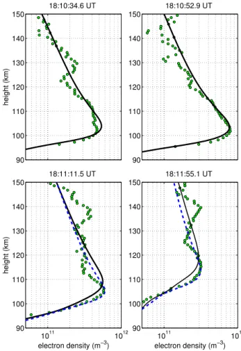
measurements are seen in individual profiles. Figure 7 is a se-lection of height profiles of measured and modelled electron densities. The first at 18:10:34 UT is during the initial stages of the run when the electron density had a clearly defined peak just above 100 km. The data are shown as circles, and the model as the black curve. At 18:10:52 UT this peak de-creased slightly in height, but mainly inde-creased in intensity, with electron densities approaching 1012m−3. The model
profiles make an excellent fit to the data. The profiles plotted in the lower two panels are from the interval following the bright and filamentary aurora, when there were pulsations and flickering, and very variable profiles on this time scale. In order to produce a consistent fit to all profiles, a great deal of iteration is needed. The blue dashed curve is an example of the result of increasing the monoenergetic peak energy by 3 keV at this time. The peak electron density is well fitted at 18:11:11 UT, and again at 18:11:55 UT. However, the in-crease in peak energy has changed the shape of the resulting electron density profile above the peak. There is much short time-scale variablity in this height range. It is possible to refine the input to the model for each time step to obtain a more exact match for each profile. However, this is not the purpose of the present work, which is to give a clear indica-tion that the model reproduces the electron density profiles well in terms of total flux and peak energy.
4.2 Modelled and measured brightness
Modelled brightnesses for the three ASK emissions are shown in Fig. 8 as blue curves. These are compared with measured brightnesses from each ASK camera, which have been spatially integrated over the radar field of view, and time integrated over 0.44 s. In the top panel, the N2 result
from ASK1 is in very good agreement throughout, with a near-constant ratio of measured to modelled brightness. As discussed in the companion paper (Ashrafi et al., 2009) there is an uncertainty resulting from the cross section used in the modelling, which can easily account for the small difference seen here. The O+ modelled brightness is compared with
90 100 110 120 130 140 150
18:10:34.6 UT
height (km)
90 100 110 120 130 140 150
18:10:52.9 UT
1011 1012
90 100 110 120 130 140 150
18:11:11.5 UT
electron density (m−3)
height (km)
1011 1012
90 100 110 120 130 140 150
18:11:55.1 UT
electron density (m−3)
Fig. 7.Comparison of individual profiles of modelled electron den-sity with radar measured profiles.
ASK2 measurements in the second panel. The measured val-ues are very small in these events, below 100 R. Under these conditions, the subtraction of the background and any con-tamination becomes a very important consideration. Never-theless, the results are very good; since they are not the sub-ject of this paper, they are not discussed further. The third panel contains the measured brightness from ASK3 of the OI emission in red. Here the model results are divided into two contributions: from excitation of atomic oxygen in light blue, and from dissociation of O2in dot-dash. The total brightness
is in dark blue, and shows a very good agreement.
4.3 Ratio of OI/N2brightness
The object of this modelling study is to validate the use of the ratio of OI/N2emission rates to estimate the variations in
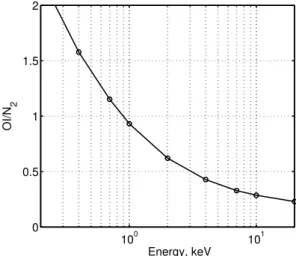
energy of precipitation within the small field of view of the ASK cameras at high temporal resolution. A demonstration of how this ratio varies with energy is given in Fig. 9, which shows modelled OI/N2 brightness plotted as a function of
energy for a constant input flux (here 2 mW/m2). There is a
10:30 11:00 11:30 12:00 0
2000 4000 6000 8000
Brightness (R)
10:30 11:00 11:30 12:00
0 100 200 300 400 500
Brightness (R)
10:30 11:00 11:30 12:00
0 500 1000 1500 2000
Brightness (R)
Minutes after 18 UT ASK1 model N
2
ASK2
model O+
ASK3 model OI
model OI−D model OI+OI−D
Fig. 8. Comparison of measured and modelled emission bright-nesses for the three ASK cameras.
Such a graph can be used as a “look-up table” for energy, converting measured ratios to energy. It can be seen that the graph is particularly sensitive to variations in energy below a few keV. In the events used in the above modelling, the peak energy of precipitation was above 1 keV throughout, and for the monoenergetic distribution was mostly greater than 4 keV. This interval of high energy precipitation was chosen since it allowed the electron density profiles from the radar to be fitted with the least uncertainty. The profiles had clear peaks in the E region which mostly were well-fitted to a dominant distribution of monoenergetic electrons.
Although the real power of the technique described is for detecting low energy precipitation, it is nevertheless possible to discriminate between different energies within the auro-ral signatures observed here. In the event chosen, the anal-ysis has been based on radar measurements which have a time resolution of 0.44 s. The auroral changes are very much faster than this, and with the ASK instrument, measurements are made at up to 32 frames per second. The corresponding energy changes can therefore be estimated at much higher temporal resolution than in the above analysis. Similarly the spatial integration used in the above work corresponds to the radar field of view. However, it is possible to obtain infor-mation about the energy and flux at a spatial resolution cor-responding to the smallest auroral features.
As an example of the technique, the changes associated with the passage of the sequence of auroral curls shown in Fig. 4 have been studied. (A movie of the event is available
100 101
0 0.5 1 1.5 2
Energy, keV
OI/N
2
Fig. 9. Modelled OI/N2ratio vs peak monoenergetic energy with input flux of 2 mW/m2.
0.3 0.4 0.5
ASK3/ASK1 ratio
a)
radar FOV 16x16 pixels
1000 2000 3000
ASK1 (R)
b) radar FOV
16x16 pixels
08:06 08:08 08:10 08:12
200 400 600
Minutes after 18 UT
ASK3 (R)
c)
radar FOV
16x16 pixels
Fig. 10. (a) Measured OI/N2 ratio(b)brightness of ASK1 and
(c)ASK3, from 18:08:05 UT to 18:08:14 UT, at two spatial reso-lutions: the field of view of radar (black) and 16×16 pixels in the magnetic zenith (grey). (bottom) Images 250 ms apart starting at 18:08:09 UT as marked in (b).
as supplementary material: http://www.ann-geophys.net/27/ 2881/2009/angeo-27-2881-2009-supplement.zip.) The first approach is to study the temporal changes within the images, using different spatial resolutions. The top panel of Fig. 10 is a short time series of the measured OI/N2brightness
at 100 km height, which is still larger than the smallest fea-tures observed. For comparison the changes within the field of view of the radar are included (black curve). The rela-tive sizes of these fields of view are shown in the images below. The second and third panels are the brightnesses of both ASK1 and ASK3 during the same sequence, and at the same two spatial resolutions. A clear observation is that the fourth curl at 18:08:11 UT is not measured in the zenith, but it is contributing to the signal in the wider integration region. Examination of the images at this time resolution shows that the fluctuations in the emissions within each curl are significant. The images in the bottom row of Fig. 10 show the passage of the third curl at 18:08:09 UT, over 1 s. The times of the images are marked with arrows on the second panel, which is the N2brightness, and thus directly related
to the flux. The images are separated by 250 ms showing the changes in intensity within the thin filament as it winds and unwinds. The first arrow corresponds to the abrupt change as the narrow feature enters the small field of view. There are clear changes in brightness within each part of the wind-ing structure, such that the selected ASK measurements are a combination of spatial and temporal changes. At the time of the second arrow, a sudden brightening of the narrow fila-ment has moved through the smaller field of view. Following this the narrow gap between the curling filaments is mea-sured. The brightest part of the structure is often outside the selected area, as seen at the time of the third arrow, when the inner filament in the narrow field of view is weaker than the outer filament. At the time of the final arrow most of the curl feature has moved out of the selected region. The observed OI/N2ratio varies between 0.2 in the bright filaments and 0.4
in the region outside the curl. From Fig. 9 these values corre-spond to peak energies in the region of 20 keV within the curl and energies of 5–10 keV outside the bright feature. Values of flux are estimated from the N2 brightness in the smaller
zenith field of view. As the curl enters this region the flux increases from approximately 3 mW/m2to 7 mW/m2.
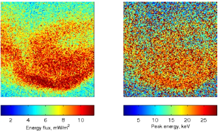
Another approach is to study the spatial changes across the images, rather than the changes within the magnetic zenith as demonstrated above. The sequence shown in Fig. 10 is a combination of both temporal and spatial changes. The whole event is associated with a region of mainly high en-ergy precipitation. In such events, assuming that most of the emission originates from a narrow region in height, it is pos-sible to use the variation in the ratio across each image to estimate changes in energy. This method has been demon-strated by Dahlgren et al. (2008a), who have used ASK data to study the changes in the ratio of O+2/OI across images of different auroral features. In one case of a curling narrow arc, similar in appearance to that shown here, the ratio was ap-proximately constant across the whole image, implying that the changes within the feature were all caused by changes in flux, rather than energy. In the narrow curling feature within the present data, we find that flux and energy are clearly cou-pled. In Fig. 11 images from ASK1 have been converted into
Fig. 11. Images of ASK 1 and measured OI/N2ratio at 18:08:09, converted into energy flux and peak energy respectively.
values of flux, using the factor described in Sect. 4.1 and the ratios of ASK3/ASK1 have been converted into energy, us-ing the relationship of Fig. 9. This spatial approach must be treated with caution, as the interpretation of brightness when measured off-zenith is sensitive to even angles of less than a degree away from the field-aligned direction. It is only pos-sible to consider this approach in the present event because the energies are uniformly high, giving large values of the ratio. Future work will investigate very sharp boundaries and extremely narrow filaments viewed out of the zenith, thus suggesting very narrow layers of emission.
5 Discussion
The purpose of the analysis described is primarily to show the value of multispectal imaging in studying auroral fine structure. The choice of filters is crucial to this work. The modelling study proves that the emission rates from atomic oxygen at 777.4 nm and molecular nitrogen at 673.0 nm can be used to estimate the energy and flux of precipitation within small structures.
The data chosen for this study are from the mainland of Norway, at the site of the EISCAT radar (69.6 N, 19.2 E). The ASK instrument spent only one winter at this location; previously and subsequently it has been at the higher latitude of Svalbard (78.1 N, 16.0 E). The auroral signatures from the mainland radar site are typical of precipitation on the night-side of the auroral oval, with high energy electrons dominat-ing the resultdominat-ing emissions. Consequently, the contributions to the optical signatures in the events discussed are mostly from electrons with energies greater than 1 keV. The tech-niques described will be most valuable when analysing data from the dayside region of the auroral oval when low energy precipitation often dominates.
from excitation of atomic oxygen, and for energies of a few keV this emission is found below heights of 150 km, as can be seen in Fig. 1. Note the different scales for the two contri-butions to 777.4 nm emission rates in this figure. The relative contribution to 777.4 nm emission rate from molecular disso-ciation is weak for these energies. In the events described, the OI/N2ratio reflects relatively small changes in the energy of
precipitation throughout, with peak energies mostly of about 10±5 keV. In aurora where low energies dominate, as has
been found in rayed aurora (Ivchenko et al., 2004)), and in quiet arcs (Dahlgren et al., 2008b), we would expect ratios greater than unity in regions where the contribution from OI excitation dominates at heights above 200 km. Such events will be the subject of future studies.
As can be seen in Fig. 6 there are some discrepancies be-tween the modelled and measured electron densities during the latter part of the interval analysed. It is very clear that the time resolution of the radar data limits the ability to fit realis-tic profiles at all times. When the field of view of the radar is filled with aurora, the fitting is good. During the latter part of the interval, this condition is often not met, with changes in patches moving in and out of the field of view, pulsating and even flickering. The sampling time of 0.44 s is clearly far too long for aurora such as the narrow curls and filaments shown in Fig. 10, and the size of the radar field of view too large. For the short sequence including the curls it is impossible to make good fits to the radar data. However, the great advan-tage of multispectral imaging using the method described is that it allows such events to be analysed using the optical data alone.
Uncertainties in measurements which would affect the ra-tio estimara-tion are the subtracra-tion of background contamina-tion, and the absolute calibration of the imager data. The wavelength range of the filter in the case of the N2emission
is relatively free of significant emissions which could con-taminate the results. The main contribution is from bands of the N+2 Meinel and O+2 1N. Referring to Fig. 4.5 of Vallance-Jones (1974), the contribution from N+2 Meinel (7,3) and (8,4) and other emissions including O+2 1N (2,4), (1,3), and (0,2) is at most 10–15% in the wavelength range of the filter transmission. In the OI filter range, there is a small contri-bution (less than 10%) from N21P bands, which would cause
a small shift in the ratio curve (note the OI filter width is 1.5 nm compared with 14 nm for the N2). The uncertainty
arising from the calibration process has not been quantified for the present work.
Uncertainties arising from the model include the choice of cross sections which, for the case of the N2 emission,
have been considered in detail in Ashrafi et al. (2009). Lum-merzheim and Lilensten (1994) have discussed errors in the transport model and estimated uncertainties of the order of 15–20%, which would be increased with uncertainty of the atmospheric conditions. These may change significantly in the F region during auroral activity, such that the MSIS-90
model values used as input may not be completely suitable. Joule heating by electrojets in the auroral region can cause upwelling of neutrals, depleting the relative density of atomic oxygen in the E region. This will cause changes to the rela-tive production rates of ions from each of the neutral species. However, such changes do not significantly affect ionisation rate profiles in the lower E region where the present measure-ments are made (Palmer, 1995).
When estimating the energy flux using both radar and op-tical methods, the size of the field of view used has a signif-icant effect. For the optical data a very small field of view is possible. When there is strong aurora, even a pixel by pixel approach can be used. For the present data it was consid-ered that the field of view of 16×16 pixels was optimal. The uncertainties that arise from using Fig. 9 to convert the ra-tio of OI/N2to energy are large when estimating energies in
the high energy part. Not only is the slope of the graph very shallow, making a determination of an energy very rough, but the assumptions that are inherent in the graph are significant. The actual energy distributions at any time are not a simple gaussian shape, nor is the energy flux a constant value. In fact there is a weak dependence of energy on flux. Never-the-less the approach demonstrated here provides a straightforward method of determining the dominant energy of precipitation.
6 Conclusions
Results from the ASK instrument have confirmed that mul-tispectral imaging is a powerful tool in estimating the fast changes in energy distributions within the smallest auroral structures.
Electron density profiles from E region incoherent scat-ter radar have been used to estimate input energy spectra for modelling the observed emission rates. Estimates of the time-varying energy flux, using both radar and optical meth-ods, have been shown to be excellent, in particular when the aurora filled the radar field of view. Detailed modelling of individual height profiles can be performed to great accuracy within the time and space resolution of the radar data.
The motivation for the three filters used on the ASK in-strument has been described, with particular emphasis on the choice of the atomic oxygen filter at 777.4 nm. Modelling of the three emissions has been successfully performed, con-firming that the cross sections used for each emission in the model are reasonable.
within narrow structures. For high energy precipitation it has been shown that spatial variations in energy and flux can be made with a pixel by pixel analysis, providing even higher spatial resolution for these events.
Future studies will make use of the method described for studying low energy precipitation in the cusp region, and in the dayside aurora measured on Svalbard, where the ASK instrument is now installed, close to the EISCAT Svalbard Radar, and the Spectrographic Imaging Facility (University of Southampton) which adds valuable wavelength informa-tion to support the ASK measurements. This combinainforma-tion of instruments promises to be most fruitful for determining the processes that accelerate electrons into the atmosphere, pro-ducing the complex forms and shapes of the aurora. For ex-ample, in several events under investigation there are found to be very clear spatial discontinuities in the ratio across the zenith field of view, indicating very sharp boundaries in the distributions reaching the upper atmosphere.
Acknowledgements. The ASK instrument was funded by the PPARC of the UK. MA is supported by the STFC. NI is sup-ported by the Swedish Research Council (VR). EISCAT is an inter-national association supported by research organisations in China (CRIRP), Finland (SA), France (CNRS, till end 2006), Germany (DFG), Japan (NIPR and STEL), Norway (NFR), Sweden (VR), and the United Kingdom (STFC). We thank the EISCAT and ASK campaign teams for running the instruments. In particular we thank Bjorn Gustavsson for invaluable help in setting up the ASK instru-ment for the season. We thank Daniel Whiter, Olli Jokiaho and Dirk Lummerzheim for help with modelling and analysis and for useful scientific discussions.
Topical Editor M. Pinnock thanks S. Okano and J. Semeter for their help in evaluating this paper.
References
Ashrafi, M., Lanchester, B. S., Lummerzheim, D., Ivchenko, N., and Jokiaho, O.: Modelling of N21P emission rates in aurora using various cross sections for excitation, Ann. Geophys., 27, 2545–2553, 2009, http://www.ann-geophys.net/27/2545/2009/. Christensen, A. B., Rees, M. H., Romick, G. J., and Sivjee, G. G.:
OI (7774 ˚A) and OI (8446 ˚A) emissions in aurora, J. Geophys. Res., 83, 1421–1425, 1978.
Dahlgren, H., Ivchenko, N., Lanchester, B. S., Sullivan, J., Whiter, D., Marklund, G., and Strømme, A.: Using spectral characteris-tics to interpret auroral imaging in the 731.9 nm O+line, Ann. Geophys., 26, 1905–1917, 2008a,
http://www.ann-geophys.net/26/1905/2008/.
Dahlgren, H., Ivchenko, N., Sullivan, J., Lanchester, B. S., Mark-lund, G., and Whiter, D.: Morphology and dynamics of aurora at fine scale: first results from the ASK instrument, Ann. Geophys., 26, 1041–1048, 2008b,
http://www.ann-geophys.net/26/1041/2008/.
Dahlgren, H., Ivchenko, N., Lanchester, B. S., Ashrafi, M., Whiter, D. K., Marklund, G., and Sullivan, J. M.: First direct optical observations of plasma flows using afterglow of O+in discrete aurora, J. Atmos. Sol. Terr. Phys., 71, 228–238, 2009.
Erdman, P. W. and Zipf, E. C.: Excitation of the OI (3s5S0-3p5P) λ7774 ˚A multiplet by electron impact on O2, J. Chem. Phys., 87, 4540–4545, 1987.
Gulcicek, E. E., Doering, J. P., and Vaughan, S. O.: Absolute differ-ential and integral electron excitation cross sections for atomic oxygen. VI – The3P -3P and3P –5P transitions from 13.87 to 100 eV, J. Geophys. Res., 93, 5885–5889, 1988.
Gustavsson, B., Steen, A., Sergienko, T., and Br¨andstr¨om, B. U. E.: Estimate of auroral electron spectra, the power of ground-based multi-station optical measuremnts, Phys. Chem. Earth (C), 26, 189–194, 2000.
Hecht, J. H., Christensen, A. B., and Pranke, J. B.: High-resolution auroral observations of the OI(7774) and OI(8446) multiplets, Geophys. Res. Lett., 12, 605–608, 1985.
Hedin, A. E.: Extension of the MSIS Thermospheric Model into the Middle and Lower Atmosphere, J. Geophys. Res., 96, 1159– 1172, 1991.
Ivchenko, N., Rees, M. H., Lanchester, B. S., Lummerzheim, D., Galand, M., Throp, K., and Furniss, I.: Observation of O+(4
P-4D0) lines in electron aurora over Svalbard, Ann. Geophys., 22,
2805–2817, 2004, http://www.ann-geophys.net/22/2805/2004/. Julienne, P. S. and Davis, J.: Cascade and radiation trapping effects
on atmospheric atomic oxygen emission excited by electron im-pact, J. Geophys. Res., 81, 1397–1403, 1976.
Lanchester, B. S., Rees, M. H., Lummerzheim, D., Otto, A., Frey, H. U., and Kaila, K. U.: Large fluxes of auroral electrons in fila-ments of 100 m width, J. Geophys. Res., 102, 9741–9748, 1997. Lanchester, B. S., Rees, M. H., Sedgemore, K. J. F., Palmer, J. R., Frey, H. U., and Kaila, K. U.: Ionospheric response to variable electric fields in small-scale auroral structures, Ann. Geophys., 16, 1343–1354, 1998,
http://www.ann-geophys.net/16/1343/1998/.
Lanchester, B. S., Lummerzheim, D., Otto, A., Rees, M. H., Sedgemore-Schulthess, K. J. F., Zhu, H., and McCrea, I. W.: Ohmic heating as evidence for strong field-aligned currents in filamentary aurora, J. Geophys. Res., 106, 1785–1794, 2001. Lummerzheim, D. and Lilensten, J.: Electron transport and energy
degradation in the ionosphere: evaluation of the numerical solu-tion, comparison with laboratory experiments and auroral obser-vations, Ann. Geophys., 12, 1039–1051, 1994,
http://www.ann-geophys.net/12/1039/1994/.
Palmer, J.: Plasma density variations in the aurora, PhD thesis, 1995.
Schulman, M. B., Sharpton, F. A., Chung, S., Lin, C. C., and Ander-son, L. W.: Emission from oxygen atoms produced by electron-impact dissociative excitation of oxygen molecules, Phys. Rev. A, 32, 2100–2116, 1985.
Semeter, J., Lummerzheim, D., and Haerendel, G.: Simultaneous multispectral imaging of the discrete aurora, J. Atmos. Sol. Terr. Phys., 63, 1981–1992, 2001.
Vallance-Jones, A.: Aurora, Cambridge University Press, 1974. Zipf, E. C. and Erdman, P. W.: Electron impact excitation of atomic