Evaluation of OSEB and SEBAL models for energy balance of a crop area in a humid subtropical climate

(1)

ABSTRACT: This study evaluated the adequacy of the One-Source Energy Balance (OSEB) and Surface Energy Balance Algorithm for Land (SEBAL) models to estimate evapotranspiration in grain growing areas with humid subtropical climate in Rio Grande do Sul, southern Brazil. The dataset was obtained from a micrometeorological station (Eddy Covariance) and MODIS (Moderate Resolution Imaging Spectroradiometer) products during 84 observation days between 2009 and 2011. The OSEB and SEBAL models were used to estimate the partition of net radiation (Rn) into the components latent heat flux (LE), sensible heat flux (H), and ground heat flux (G) estimated from the MODIS images while the experimental data measured in situ

AGROMETEOROLOGY - Article

Evaluation of OSEB and SEBAL models for

energy balance of a crop area in a humid

subtropical climate

Juliano Schirmbeck1_{*, Denise Cybis Fontana}2_{, Débora Regina Roberti}3

1.Universidade Federal do Rio Grande do Sul - Centro Estadual de Pesquisas em Sensoriamento Remoto e Meteorologia - Porto Alegre (RS), Brazil.

2.Universidade Federal do Rio Grande do Sul - Faculdade de Agronomia - Porto Alegre (RS), Brazil. 3.Universidade Federal de Santa Maria - Departamento de Física - Santa Maria (RS), Brazil.

*Corresponding author: schirmbeck.j@gmail.com Received: June 23, 2017 – Accepted: Jan. 2, 2018

(2)

INTRODUCTION

The correct understanding of the partitioning of energy and mass fluxes on the Earth surface is extremely important for climate, hydrological and agrometeorological studies. Nevertheless, scalar measurements of energy fluxes are generally restricted to specific points such as micrometeorological sites since measurements are costly and reliant on expensive instruments and specialized staff.

On a regional scale, Remote Sensing (RS) is an excellent tool to monitor the spatial distribution and temporal evolution of natural vegetation or agricultural crops. RS images acquired at different wavelengths allow determining the surface physical properties necessary to measure the energy and mass flux between the surface and atmosphere on a regional scale (Boegh et al. 2002; Kustas et al. 2004; Timmermans et al. 2007).

Most studies estimating the energy balance (EB) components are based on one-dimensional flux model describing the exchange mechanisms of radiation and heat fluxes between the surface and atmosphere while observing the energy conservation principle (Brutsaert 1984). The EB can be defined by how the net radiation (Rn) of the surface is divided into latent heat flux (LE), sensible heat flux to the air (H), and ground (G) (Friedl 2002; Timmermans et al. 2007), but most studies neglect the horizontal heat advection and heat storage at the canopy layer.

Most models for estimation of EB components by RS are based on the combined use of meteorological and image data. The Rn and G components are easily estimated from the RS data. Rn can be spatialized from albedo and thermal image while G is estimated as a portion of Rn, proportional to the vegetation index. Other components such as the turbulent fluxes, LE and H, are more complex to estimate. In general,

LE is obtained as a residual component from the EB equation whereas H is estimated from the thermal images. The models differ greatly in the methodology to estimate H.

The Surface Energy Balance Algorithm for Land (SEBAL) (Bastiaanssen 2000) model has been applied using images from different sensors and locations across the globe. In Rio Grande do Sul, Brazil, the SEBAL model using high-resolution images has already been applied (Santos et al. 2010; Monteiro et al. 2014). However, because it has been parameterized for semi-arid climate, its suitability for different climatic conditions must still be verified, since the method presupposes the existence of extreme water conditions. The selection of

points with extreme moisture conditions, the hot and cold pixels, is a requirement for determining H. However, this water condition requirement may not be fulfilled in many cases, especially in humid climate. Furthermore, defining these extremes is even more difficult when using images of moderate or low spatial resolution.

This study aimed at verifying the adequacy of the One-Source Energy Balance (OSEB) and SEBAL models to estimate the latent heat flux in grain producing areas in the humid subtropical climate of Rio Grande do Sul, using low-resolution MODIS (Moderate Resolution Imaging Spectroradiometer) images. The performance of the mathematical models was evaluated by comparing the results to the experimental data of the energy balance components obtained from the experimental area in Cruz Alta, Rio Grande do Sul.

MATERIAL AND METHODS

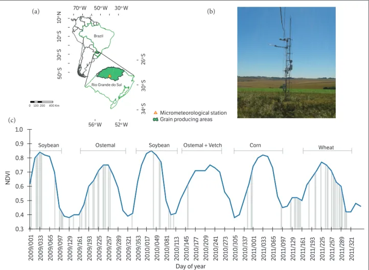
The study site is located in northwestern Rio Grande do Sul, Brazil (Fig.1). This grain producing area is greatly important to the state and country. The climate in the region is humid subtropical, classified as Cfa (according to Köppen) with highly variable rainfall and frequent droughts, which are responsible for the yield differences observed in the state.

The study period lasted three years, from 2009 to 2011. The reference data from the micrometeorological station in Cruz Alta were used to check the performance of the OSEB and SEBAL mathematical models to estimate the EB component estimates.

Over the period, 84 days were selected for analysis. The selection criteria were completely clear sky day over the area throughout the day (verified from the global solar radiation data) and the availability of MODIS products with adequate quality. The analyzed dates were distributed over the period of three years, which allowed analyzing the models in various weather conditions. Of the analyzed dates/images, 20 corresponded to summer crops, 32 winter crops, and 32 partial vegetation cover. The NDVI profile pattern \and analyzed dates (Fig. 1c) were distributed to represent the variability of results according to time of year/season, crop type, and degree of surface coverage.

(3)

and H, is more complex. In most EB models, LE is obtained as a residual term in the EB equation.

The main difference between models to estimate the EB components from remote sensing data lies in the way the sensible heat flux (H) is determined. Among them, three approaches are highlighted. In fact, the OSEB models are based directly on the radiometric temperature difference between the vegetated surface and air temperatures (Boegh et al. 2002; Friedl 2002, Kustas et al. 2004, Wang et al. 2006; Sánchez et al. 2008; Timmermans et al. 2007; Tang et al. 2013). Likewise, the TSEB (Two-Source Energy Balance) models treat differently the heat exchange between the atmosphere and vegetated areas, and between the atmosphere and areas with bare soil based on different equations to determine the components in soil and vegetated areas (Sánchez et al. 2008, Cammalleri et al. 2012, Tang et al. 2013). Finally, the third approach, the SEBAL (Surface Energy Balance Algorithm for Land) (Bastiaanssen 2000), the SSEBI (Simplified Surface

Energy Balance Index) (Roerink et al. 2000, Mattar et al. 2014) and METRIC (Mapping Evapotranspiration with Internalized Calibration) (Allen et al. 2007) models could be considered as a subfamily of OSEB models, seeking to represent the spatial variations of the vegetation and atmosphere water availability by mapping the cold and hot image pixels. Thus characterizing, respectively, the maximum latent heat flux (LE = maximum and H = 0) and maximum sensible heat flux (LE = 0 and H = maximum).

The studied (OSEB and SEBAL) models are based on the principle of energy conservation, Brutsaert (1984) (Eq. 1):

Rn + G + H + LE ≈ 0 (1)

The first term of the EB equation, net radiation (Rn), can be estimated from the satellite images using Eq. 2:

Rn = R_G↓(1 – α) + εsεaσT 4 a – εsσT

4

s (2) Figure 1. Spatial and temporal scales of the study; (a) site location in Rio Grande do Sul, Brazil; (b) micrometeorological station; (c) dates of the images selected for analysis over the three-year period (gray lines) and NDVI in Cruz Alta experimental site.

Soybean Ostemal Soybean Ostemal + Vetch Corn _Wheat

Day of year 0.3 0.4 0.5 0.6 0.7 0.8 0.9 1.0 ND VI 2 009 /001 2 009 /0 3 3 2 009 /065 2 009 /09 7 2 009 /1 2 9 2 009 /1 6 1 2 009 /1 9 3 20 0 9 /2 25 20 0 9 /25 7 2 009 /2 8 9 2 009 /3 2 1 2 009 /3 5 3 2 010 /01 7 2 010 /04 9 2 010 /081 20 10/ 113 2 010 /1 45 20 10/ 17 7 20 10/ 20 9 20 10/ 2 4 1 2 010 /2 73 2 010 /3 05 20 10/ 3 3 7 2 01 1/ 001 2 01 1/ 0 3 3 2 01 1/ 065 2 01 1/ 09 7 2 01 1/ 12 9 2 01 1/ 16 1 2 01 1/ 19 3 20 11 /2 25 20 11 /25 7 2 01 1/ 2 8 9 2 01 1/ 3 2 1 Micrometeorological station Grain producing areas Rio Grande do Sul

Brazil

0 100 200 400 Km

56o _W

30o _W

50o _W

70o _W

52o _W

34

o S

30

o S

26

o S

50

o S

30

o S

10

o S

10

o N

(a) (b)

(4)

where: R_G↓ is the global solar radiation (MJ·m–2_·day–1_);

a is the surface albedo (dimensionless); εs is the surface

emissivity (dimensionless); εa is the atmosphere emissivity

(dimensionless); s is the Stefan-Boltzmann constant (4.9 × 10–9_MJ·m–2_·K–4_·day–1_);_T

a is the air temperature (K);

and Ts is the surface temperature (K).

The a, Ts, and εsparameters were determined from remote

sensing thermal images while the other components from the experimental data obtained at the micrometeorological station (Boegh et al. 2002; Sobrino et al. 2005; Rivas and Caselles 2004).

For the OSEB and SEBAL models, the latent heat flux,

LE, was estimated as the residual term of Eq. 1.

The main difference between models OSEB and SEBAL models is how the third term of the EB equation, the sensible heat flux to the atmosphere H, which represents the portion of absorbed radiation released as heat from the surface to the air, is determined. Both models estimate H from a temperature differential and aerodynamic resistance, according to Eq. 3:

H = ρcp × dT/ra (3)

where: ρ is the air density (1.15 Kg·m–3_);_cp_{(1004 J·Kg}–1_·K–1₎

is the specific heat of humid air at constant pressure; dT is the differential temperature between two levels on the surface; and ra is the aerodynamic resistance to heat transport (s·m–1_).

In the OSEB model, the differential temperature, dT, is the difference between surface (obtained from satellite image) and air temperatures, normally obtained from meteorological stations at 2 m above the surface (Boegh et al. 2002; Kustas et al. 2004; Wang et al. 2006), and ra is obtained from wind speed according to Allen et al. (1998).

For the SEBAL model, the differential temperature and aerodynamic residence are obtained from an iterative calculation procedure, which seeks atmospheric stability condition for each image pixel, based on anchor pixels that represent the extreme soil moisture of the image. The detailed methodology for obtaining these parameters is explained by Bastiaanseen (1995).

In both models, ground heat flux G is estimated as a fraction of Rn, inversely to the vegetation indices (Allen 1998; Boegh et al. 2002; Qi et al. 1994; Moran et al. 1989). In the OSEB model, G is estimated from Eq. 4 (Moran et al. 1989):

G = 0.583exp(–2.13NDVI)Rn (4)

The SEBAL model estimates G from NDVI, but it adds the albedo (α) and surface temperature (Ts) data using Eq. 5

(Bastiaanssen 2000):

G = [(Ts/α)(0.0038α + 0.0074α)(1– 0.98NDVI4_)]_Rn₍₅₎

The EB components were obtained from the MODIS products: Earth surface temperature – MOD11A2; vegetation index – MOD13A2; Albedo – MCD43B3; and leaf area index – MOD15A2. All used products had 1,000 m spatial resolution while temporal resolutions consisted of temporal compositions of 16 days for MOD13, 8 days for MCD43B3 and MOD15A2, and daily for MOD11A2.

These products are available as daily scenes covering a specific area of the globe. A mosaic of the H13V11 and H13V12 sinusoidal tiles, obtained from the Land Processes Distributed Active Archive Center website (https://lpdaac.usgs.gov), was prepared to cover the study site.

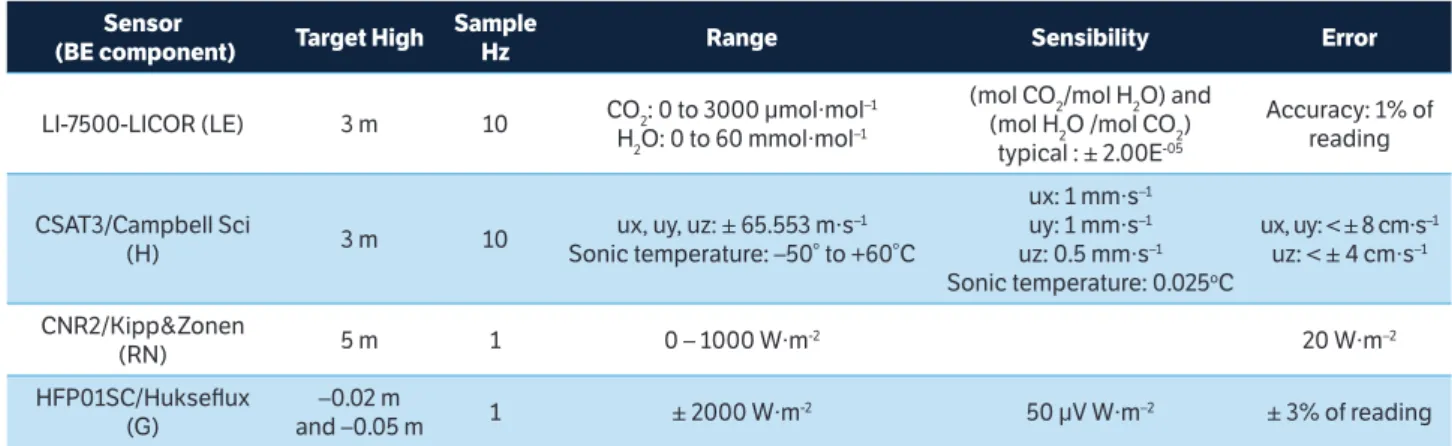
The EB components were obtained experimentally at 3 m high, using the data collected from the microteorological station, equipped with net radiation sensor (Rn), ground heat flux sensor (G), measuring in low frequency 1 Hz, 3D sonic anemometer and infrared gas analyzer measuring in high frequency (10 Hz). The turbulent fluxes of sensible (H) and latent heat (LE) were estimated by the Eddy Covariance method, obtaining 30 min averages. The EB sensor has been described in Table 1. The station have other sensors to measure atmospheric pressure, rainfall, shortwave incident radiation, photosynthetically active radiation, and soil temperature.

The Eddy Covariance system estimates all EB components independently, generally the (LE + H) is different from the available energy (Rn – G) and should be adjusted to close the EB. The method applied to close the EB is based on maintaining the Bowen Ratio while the available surface energy is re-partitioned (Tang et al. 2013).

(5)

The model results (average of 3 × 3 pixel window centered at the micrometeorological station) were compared with the reference measurements performed at the micrometeorological station. Those analyses were performed using dispersions for both component and model. The quality of the estimates was checked by the Root Mean Square Error (RMSE), Mean Bias Error (MBE, computed as observed – estimated), and the analysis of the EB component ratios in relation to Rn.

RESULTS AND DISCUSSION

Partition of the EB components – experimental data

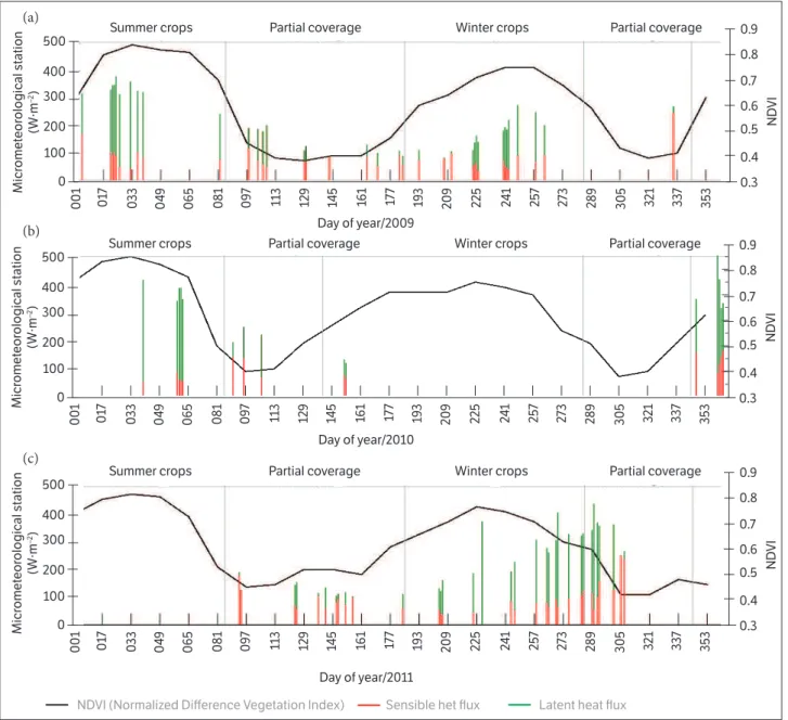
The pattern of EB components measured in the micrometeorological station is shown in Fig. 2. These plots show the mean data recorded every half hour during 20 random days in the summer crops (Fig. 2a), 32 in the winter crops (Fig. 2b), and 32 days over partial vegetation cover (Fig. 2c). The EB closure has been applied to this data.

The results for the energy balance components showed higher Rn values for the summer crops (Fig. 2a), lower and similar for the winter crops (Fig. 2b) and partial vegetation cover (Fig. 2c). The results for the energy balance components showed that Rn was higher for the summer crops (Fig. 2a), and lower and similar for the winter crops (Fig. 2b) and partial vegetation cover (Fig. 2c). The highest energy input varied between 796 W∙m–2_{and 580 W∙m}–2_{, with mean of 698 W∙m}–2

in the summer, and between 744 W∙m–2_{and 302 W∙m}–2_{, with}

mean of 474 W∙m–2_{in the winter; these measurements were}

recorded at 12:30 PM (local time) when available radiation is maximized. The observed values for Rn and LE, H and

G fluxes are associated with the subtropical climate of the study area and varying coverage over time.

Table 1. Specifications of sensor BE components installed at the micrometeorological station in Cruz Alta. Sensor

(BE component) Target High

Sample

Hz Range Sensibility Error

LI-7500-LICOR (LE) 3 m 10 CO2: 0 to 3000 μmol∙mol

–1

H₂O: 0 to 60 mmol∙mol–1

(mol CO₂/mol H₂O) and

(mol H₂O /mol CO₂)

typical : ± 2.00E-05

Accuracy: 1% of reading

CSAT3/Campbell Sci

(H) 3 m 10

ux, uy, uz: ± 65.553 m∙s–1

Sonic temperature: –50° to +60°C

ux: 1 mm∙s–1

uy: 1 mm∙s–1

uz: 0.5 mm∙s–1

Sonic temperature: 0.025o_C

ux, uy: < ± 8 cm∙s–1

uz: < ± 4 cm∙s–1

CNR2/Kipp&Zonen

(RN) 5 m 1 0 – 1000 W∙m-2 20 W∙m–2

HFP01SC/Hukseflux (G)

–0.02 m

and –0.05 m 1 ± 2000 W∙m-2 50 μV W∙m–2 ± 3% of reading

Figure 2. Experimental average daily cycle of the components of the energy balance in Cruz Alta, Rio Grande do Sul, Brazil; (a) summer crops; (b) winter crops and (c) partial vegetation coverage.

Satellite overpass time

(76% of Rn)

(19% of Rn)

(5% of Rn)

800 700 600 500 400 300 200 100

0 –100

00:30 03:30 06:30 09:30 12:30 15:30 18:30 21:30

(61% of Rn) (21% of Rn) (18% of Rn)

800 700 600 500 400 300 200 100

0 –100

00:30 03:30 06:30 09:30 12:30 15:30 18:30 21:30

(52% of Rn) (41% of Rn)

(8% of Rn)

800 700 600 500 400 300 200 100

0 –100

00:30 03:30

Latent heat flux Net radiation Ground heat flux Sensible heat flux

06:30 09:30 12:30 15:30 18:30 21:30

(a)

(b)

(6)

Figure 1c shows that the summer crop cycles were shorter and had higher NDVI, which resulted from the higher energy availability, rapid vegetation development, and higher biomass accumulation. The opposite was observed in the winter crops. In the partial vegetation coverage period, the increasing albedo resulted from more exposed soil, senescent vegetation, which increased short-wave radiation loss and provided Rn value similar to winter crops (Fig. 2), with lower energy input.

At the time of the satellite overpass (Table 2), the Rn

partition was similar to that observed throughout the day. This effect is called evaporative fraction self-preservation, providing, under some circumstances, the tool to extrapolate from instantaneous satellite retrievals to daily estimates of evapotranspiration (Cragoa and Brutsaert 1996; Cammalleri et al. 2014). The largest partition of energy is consumed by the latent heat flux, followed by sensible heat flux in the air and soil (Fig. 2).

As already mentioned, the evapotranspiration process consumes the most Rn due to the humid subtropical climate of the region. However, despite the damp climate, soil water availability is often insufficient to meet the evaporative demand of summer crops, and drought becomes responsible for yield variability hence the need to quantify it. For these same crops, the sensible heat flux, H, was the second component with the highest portion of available energy.

The highest H values were observed during the partial vegetation cover period while LE decreased (Fig. 2). This significant decrease of the LE component is possibly due to senescent vegetation accumulated on the ground since straw creates an insulating layer, partially interrupting the soil evaporation process. The soil heat flux, which is usually responsible for lower energy consumption, was lower than 8% for all crops.

Figure 3 shows how Rn was split between the LE and

H fluxes in all analyzed dates (the graphs show H + LE). For most dates, LE is higher than H, consistent with the pattern observed in the mean values. However, for a few

days, especially between the 97 and 145 days at the end of the summer crops of 2009 and 2010, H was higher than

LE. Variations were observed only in the Rn partition proportions, a result of the variable weather conditions and soil water availability. Also, it is noteworthy that the

LE and H values are close in the initial phase of winter crops.

Partition of the EB components – the OSEB and SEBAL models

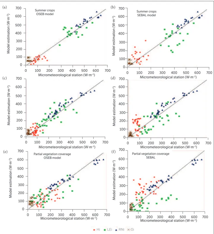
The experimental energy balance components were used as a reference for understanding how Rn partition varies over time, and the factors influencing it. The objective of this study was to determine reliable methods, mathematical models, to estimate EB from satellite images to allow drawing up maps showing the spatiotemporal distribution of EB. Figure 4 shows the scatter plots comparing the estimated and experimental data of the EB components for the OSEB and SEBAL models. The Rn

estimated by Eq. 2 behaved similarly for both models and very close to the experimental values, with the dispersion points approaching a straight line 1:1 and RMSE equal or below 50 W∙m–2_{(Table 3) for all three vegetation covers.}

Overall, Rn is the easiest parameter to be estimated and has the lowest error in EB studies from the images. Tang et al. (2013) reported similar magnitude errors (31 W∙ m–2₎

for the OSEB model in areas with maize (summer) and wheat (winter) crops in northwestern China. Also, Timmermans et al. (2007) reported errors close to 44 W∙m–2

for the SEBAL model in pasture areas in the semi-arid and sub-humid climates of Arizona and Oklahoma, respectively, in the United States.

The estimated and experimental H values showed the highest dispersion for both models. The OSEB model, based on the differential temperature between the air and surface, and aerodynamic resistance (Allen et al. 1998; Kustas et al. 2004; Tang et al. 2013), provided low H values and close to a straight line 1:1 for the summer and winter

Table 2. Instantaneous average values of the EB components for different vegetation covers obtained experimentally in Cruz Alta, Rio Grande do Sul, Brazil. The EB closure was achieved by maintaining the Bowen Ratio (Tang et al. 2013).

Measurements (10:30)

Net Radiation (W∙m–2₎

Latent heat flux Sensible heat flux Soil heat flux Latent + Sensible + Soil heat flux

W∙m–2 _% _W∙m–2 _% _W∙m–2 _% _%

Summer crops 523 395 76 100 19 27 5 100

Winter crops 349 214 61 72 21 63 18 100

(7)

crops, with RMSE less than 51 W∙m–2 _{(Table 3). However,}

for partial vegetation cover, the estimated H had a higher dispersion and RMSE.

In the winter crops, H was estimated as 20% and 40% of Rn for the OSEB and SEBAL models, respectively. For the partial cover period, experimental H measured in the station represented only 34% of Rn and 65% of Rn in the SEBAL model, exceeding the LE values. Likewise, Timmermans et al. (2007) compared the SEBAL and TSEB models and reported that the greatest deviations in the SEBAL model occurred in areas with bare soil.

Both models estimated low G values, similar to the experimental measurements obtained in the meteorological station in Cruz Alta.

LE is obtained as a residual term in the EB Eq. 1 in both models. Therefore, its estimate is directly linked to the performance of the H estimate, which is responsible for the second largest partition of energy consumption at the surface level, and whenever the H value is underestimated, the LE value is overestimated. This was observed in the OSEB model in the summer and winter images with MBE about –40 W∙m–2_{. The SEBAL model overestimated}_H_in

500 Summer crops Micr omet eor ologic al station (W·m –2)

Partial coverage Winter crops Partial coverage

400 300 200 100 0 0.9 ND VI 3 53 3 37 32 1 30 5 28 9 27 3 2 57 24 1 22 5 20 9 193 17 7 16 1 14 5 129 11 3 0 97 081 065 0 49 03 3 0 17 001 0.8 0.7 0.6 0.5 0.4 0.3 500 Summer crops Micr omet eor ologic al station (W·m –2)

Partial coverage Winter crops

Day of year/2011 Day of year/2010 Day of year/2009

Partial coverage 400 300 200 100 0 0.9 ND VI 3 53 3 37 32 1 30 5 28 9 27 3 2 57 24 1 22 5 20 9 193 17 7 16 1 14 5 129 11 3 0 97 081 065 0 49 03 3 0 17 001 0.8 0.7 0.6 0.5 0.4 0.3

NDVI (Normalized Difference Vegetation Index) Sensible het flux Latent heat flux

Figure 3. Partition of the Energy Balance into the LE (latent heat flux) and H (sensible heat flux) components, measured with the

micrometeorological station. Sum of H_(red),LE_{(green) and NDVI (Normalized Difference Vegetation Index) profiles during the years: (a)}

(a)

(b)

(8)

the winter images or periods with partial vegetation cover, and underestimated LE, with errors up to 94 W∙m–2_MBE

(Figs. 4d and 3f show LE green points concentrated below the straight line 1:1).

The H and LE values estimated by the OSEB (Fig. 5) and SEBAL models (Fig. 6) behaved similar to the experimental data (Fig. 3). The OSEB (Fig. 5) results show that, generally,

LE is higher than H; however, this ratio was inverted

Figure 4. Scatter plots of experimental versus mathematical simulation of the energy balance components for the different vegetal covers

and the 84-day period. LE = latent heat flux; H = sensible heat flux; Rn = net radiation; and G = ground heat flux. Simulations using: (a), (c) and

(e), the OSEB model; (b), (d) and (f), the SEBAL model. The experimental values correspond to the measurements conducted in the meteorological station in Cruz Alta, Rio Grande do Sul, Brazil.

700

Summer crops OSEB model

600

500

400

300

200

100

100 200 300 400 500 600 700

Micrometeorological station (W·m–2₎

Model estimation (W·m

–2)

0

700

Summer crops SEBAL model

600

500

400

300

200

100

100 200 300 400 500 600 700

–2)

0

700

600

500

400

300

200

100

100 200 300 400 500 600 700

–2)

0

700

600

500

400

300

200

100

100 200 300 400 500 600 700

–2)

0

700

600

500

400

300

200

100

100 200 300 400 500 600 700

–2)

0

700

600

500

400

300

200

100

Hi LEi RNi Gi

200 300 400 500 600 700

–2)

0

Partial vegetation coverage OSEB model

Partial vegetation coverage SEBAL

(a)

(c)

(e)

(b)

(d)

(9)

especially at the end of the summer crops. This inversion, the H higher than LE, has also been observed during a few days in the early winter crop, but it was not observed in the micrometeorological station. At the station, we observed that LE was greater than H right after the winter crops had been implemented. This difference probably occurred because the scheduled plantings of winter crops in the region and the station footprint are not representative of the MODIS pixel area.

Unlikely, the SEBAL model estimated H higher than LE

at various times over the period analyzed (Fig. 6). Monteiro et al. (2014) used Landsat images and reported overestimated

H in four of the six images analyzed in Rio Grande do Sul, while H was higher than LE in one of the images.

In the SEBAL model, the LE and H distribution is highly dependent on the correct definition of cold (LE maximum and H zero) and hot (LE zero and H maximum) pixels. Therefore, three hypotheses have been proposed to justify the uncertainties of the SEBAL model when determining the LE

and H proportions during partial vegetation cover periods and beginning of winter crops. The first hypothesis is that the

humid climate of the study area hinders the occurrence of dry areas to the point that evapotranspiration does not occur (LE zero), especially when the images are of a low energy availability period with lower evaporative atmospheric demand. The second one is that the low spatial variability of temperature in the winter does not allow the correct determination of the extreme water conditions proposed by the model. Finally, the third hypothesis is that the 1,000 m spatial resolution of the MODIS sensor for the thermal bands homogenizes the temperature patterns, making it difficult to locate the small areas with appropriate water conditions to determine the hot and cold pixels.

The spatial resolution hypothesis has also been addressed by Kustas et al. (2004). These authors analyzed how image spatial resolution affects the different EB components and found that lower spatial resolution has more influence in the H estimation. The study showed that a particular area, with 120 m pixel, has coefficient of variation 0.42, while the same area imaged with 960 m pixel (approaching the 1,000 m of this study) lowers the coefficient of variation to only 0.26, increasing the average H value of the area.

Table 3. Energy balance components estimated using the OSEB and SEBAL models, extracted from the images in the coordinates of the meteorological station in Cruz Alta, Rio Grande do Sul, Brazil.

Net radiation*

OSEB SEBAL

Latent heat flux

Sensible heat flux

Ground heat flux

Latent heat flux

Sensible heat flux

Ground heat flux

Summer crop

Mean 543 405 70 67 358 129 56

% Net radiation 75 13 12 66 24 10

SD 58 59 30 19 96 66 20

RMSE (W∙m–2₎ ₃₈ ₅₁ ₅₁ ₅₀ ₁₀₄ ₇₈ ₄₂

MBE (W∙m–2₎ _–20 _–11 ₃₁ _–40 ₃₇ _–28 _–29

Winter crop

Mean 386 254 79 54 198 156 32

% Net radiation 66 20 14 51 40 8

SD 103 97 42 19 109 64 16

RMSE (W∙m–2₎ ₅₀ ₁₀₁ ₄₅ ₃₉ ₁₀₇ ₁₀₉ ₆₈

MBE (W∙m–2₎ _–37 _–40 _–7 _–32 ₁₆ _–84 ₃₁

Partial coverage

Mean 385 164 133 89 84 249 52

% Net radiation 42 34 23 22 65 13

SD 119 96 68 33 62 79 26

RMSE (W∙m–2₎ ₅₀ ₈₉ ₆₅ ₆₈ ₁₄₈ ₁₂₁ ₃₅

MBE (W∙m–2₎ _–22 ₁₄ ₂₄ _–60 ₉₄ _–93 _–23

(10)

Similarly, Roerink et al. (2000) addressed the deficiency of using NOAA or MODIS images with large pixels, which reflect a combination of different surfaces, hindering the occurrence of pixels with extreme water conditions.

Figure 7 shows the temperature histograms of MODIS images for two of the studied days, 129/2009 and 290/2011, which are examples of the effects related to the homogenization of surface temperature patterns observed in one 1-km pixel and low winter temperature range that hinder the correct partition between LE and H in the SEBAL model. In both cases, the temperature variation between the cold (vertical

blue line) and hot (vertical red line) pixels of the image was approximately 10 °C. The temperature of the reference pixels (vertical black line) is close to the maximum temperature of the image. Given that the LE and H proportions are distributed between the hot and cold limits of the image, the proximity of the station portion with the maximum temperature causes the SEBAL model to overestimate H.

The authors suggest further studies to test whether models such as the TSEB, which are independent of determining the hot and cold pixels, could provide good estimation of the EB parameters for the humid climate of the region.

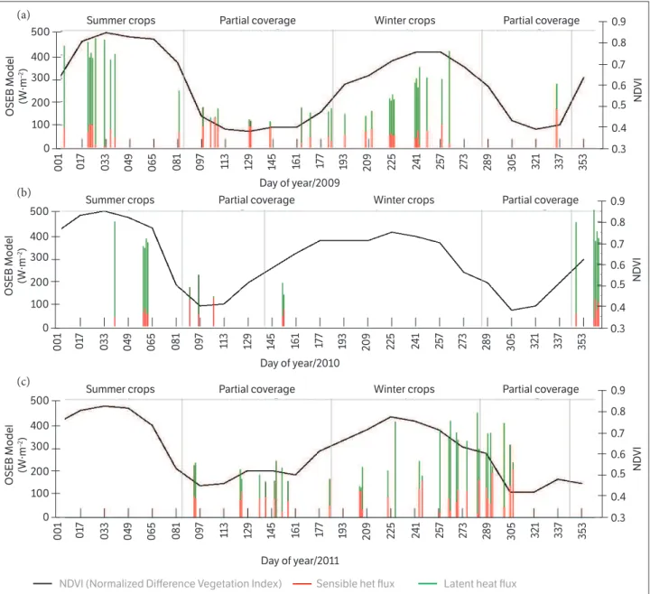
Figure 5. Partition of the Energy Balance into the LE (latent heat flux) and H (sensible heat flux) components, estimated using the OSEB.

experimental site in Cruz Alta, Rio Grande do Sul, Brazil. 500

Summer crops

OSEB Model

(W·m

–2)

400 300 200 100 0 0.9 ND VI 3 53 3 37 32 1 30 5 28 9 27 3 2 57 24 1 22 5 20 9 193 17 7 16 1 14 5 129 11 3 0 97 081 065 0 49 03 3 0 17 001 0.8 0.7 0.6 0.5 0.4 0.3 500 Summer crops OSEB Model (W·m –2)

(a)

(b)

(11)

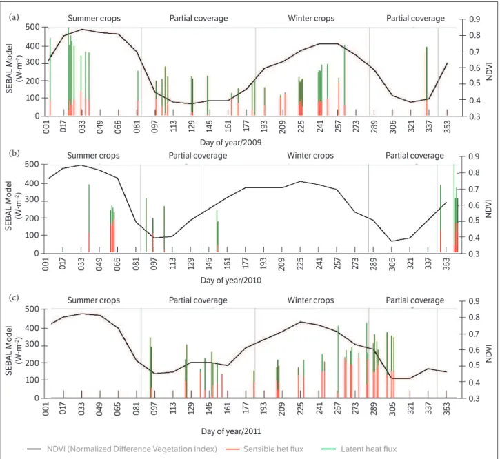
Figure 6. Partition of the Energy Balance into the LE (latent heat flux) and H (sensible heat flux) components, estimated using the SEBAL.

experimental site in Cruz Alta, Rio Grande do Sul, Brazil.

500

Summer crops

SEBAL Model

(W·m

–2)

400 300 200 100 0 0.9 ND VI 3 53 3 37 32 1 30 5 28 9 27 3 2 57 24 1 22 5 20 9 193 17 7 16 1 14 5 129 11 3 0 97 081 065 0 49 03 3 0 17 001 0.8 0.7 0.6 0.5 0.4 0.3 500 Summer crops SEBAL Model (W·m –2)

Figure 7. Histogram of the surface temperatures on: (a) 129/2009; and (b) 290/2011.

(a)

(b)

(c)

4.0 × 103

3.0 × 103

F

requency 2.0 × 10

3

285 290 295

Surface temperature K

300 305

1.0 × 103

0

F

requency

285 290 295 300

Surface temperature K

305 310

2.0 × 103

4.0 × 103

6.0 × 103

8.0 × 103

1.0 × 104

1.2 × 104

1.4 × 104

0

Cold pixel temperature used by the SEBAL model (LE = RN – G and H = 0) Hot pixel temperature used by the SEBAL model (LE = 0 and H = RN – G)

Temperature of the pixels in the reference portion in Cruz Alta, Rio Grande do Sul, Brazil

(12)

CONCLUSION

Despite the limitations offered by the spatial resolution of the images, the MODIS products allow a satisfactory estimation of the EB components. The MODIS products are provided with temporal resolutions of 1, 8 and 16 days, thus enabling to obtain satisfactory instantaneous values of the components.

The SEBAL model estimated the EB components for summer crops, the period of greater interest, satisfactorily, given the greater variability of water availability in the studied area during this period. In the other studied periods, the SEBAL model had difficulty to estimate the H correctly, while the residual component LE was underestimated.

The OSEB model, despite its simplicity, has minor errors and a better partitioning of the EB components throughout

Allen, R. G., Pereira, L. S., Raes, D. and Smith, M. (1998). Crop

evapotranspiration-Guidelines for computing crop water

requirements-FAO Irrigation and drainage paper 56. FAO, 300,

D05109.

Allen, R. G., Tasumi, M. and Trezza, R. (2007). Satellite-Based

Energy Balance for Mapping Evapotranspiration with Internalized

Calibration (METRIC) – Model. Journal of Irrigation and

Drainage Engineering 133, 380-394. http://dx.doi.org/10.1061/ (ASCE)0733-9437(2007)133:4(380)

Bastiaanssen, W. G. M. (1995). Regionalization of surface flux

densities and moisture indicators in composite terrain: a remote

sensing approach under clear skies in Mediterranean climates

(PhD Thesis). Wageningen: Wageningen Agricultural University.

Bastiaanssen, W. G. M. (2000). SEBAL-based sensible and latent

heat fluxes in the irrigated Gediz Basin, Turkey. Journal of Hydrology,

229, 87-100. http://dx.doi.org/10.1016/S0022-1694(99)00202-4

Boegh, E., Soegaard, H. and Thomsen, A. (2002). Evaluating

evapotranspiration rates and surface conditions using Landsat TM

to estimate atmospheric resistance and surface resistance. Remote

Sensing of Environment, 79, 329-343. http://dx.doi.org/10.1016/ S0034-4257(01)00283-8

Brutsaert, W. (1984). Evaporation into the atmosphere. Theory,

history, and applications. Dordrecht: Reidel Publishing Company.

the year for different soil coverages. It is concluded that this model is the most suitable for longer analysis periods such as continuous monitoring or when building a time series of EB components in the climatic conditions of Rio Grande do Sul.

ORCID IDs

J. Schirmbeck

https://orcid.org/0000-0001-9342-5144

D. C. Fontana

http://orcid.org/0000-0002-2635-6086

D. R. Roberti

https://orcid.org/0000-0002-3902-0952

REFERENCES

Cammalleri, C., Anderson, M. C., Ciraolo, G., D’Urso, G., Kustas, W.

P., La Loggia, G. and Minacapilli, M. (2012). Applications of a remote

sensing-based two-source energy balance algorithm for mapping

surface fluxes without in situ air temperature observations. Remote

Sensing of Environment, 124, 502-515. http://dx.doi.org/10.1016/j. rse.2012.06.009

Cammalleri, C., Anderson, M. C. and Kustas, W. P. (2014). Upscaling

of evapotranspiration fluxes from instantaneous to daytime

scales for thermal remote sensing applications. Hydrology and

Earth System Sciences, 18, 1885-1894. http://dx.doi.org/10.5194/ hess-18-1885-2014

Cragoa, R. and Brutsaert, W. (1996). Daytime evaporation

and the self-preservation of the evaporative fraction and the

Bowen ratio. Journal of Hydrology, 178, 241-255. http://dx.doi. org/10.1016/0022-1694(95)02803-X

Friedl, M. A. (2002). Forward and inverse modeling of land surface

energy balance using surface temperature measurements. Remote

Sensing of Environment, 79, 344-354. http://dx.doi.org/10.1016/ S0034-4257(01)00284-X

Kustas, W. P., Li, F., Jackson, T. J., Prueger, J. H., MacPherson, J. L.

and Wolde, M. (2004). Effects of remote sensing pixel resolution

on modelled energy flux variability of croplands in Iowa. Remote

(13)

Mattar, C., Franch, B., Sobrino, J. A., Corbari, C., Jiménez-Muñoz,

J. C., Olivera-Guerra, L., Skokovic, D., Sória, G., Oltra-Carriò, R.,

Julien, Y. and Mancini, M. (2014). Impacts of the broadband albedo

on actual evapotranspiration estimated by S-SEBI model over an

agricultural area. Remote Sensing of Environment, 147, 23-42. http:// dx.doi.org/10.1016/j.rse.2014.02.011

Monteiro, P. F. C., Fontana, D. C., Santos, T. V. and Roberti, D. R. (2014).

Estimation of energy balance components and evapotranspiration

in soybean crop in southern Brazil using TM - Landsat 5 images.

Bragantia, 73, 72-80. http://dx.doi.org/10.1590/brag.2014.005

Moran, M. S., Jackson, R. D., Raymond, L. H., Gay, L. W. and

Slater, P. N. (1989). Mapping surface energy balance components

by combining Landsat thematic mapper and ground-based

meteorological data. Remote Sensing of Environment, 30, 77-87.

http://dx.doi.org/10.1016/0034-4257(89)90049-7

Qi, J., Chehbouni, A., Huete, A. R., Kerr, Y. H. and Sorooshian,

S. (1994). A modified soil adjusted vegetation index.

Remote Sensing Environment, 48, 119-126. http://dx.doi.

org/10.1016/0034-4257(94)90134-1

Rivas, R. and Caselles, V. (2004). A simplified equation to estimate

spatial reference evaporation from remote sensing-based surface

temperature and local meteorological data. Remote Sensing of

Environment, 93, 68-76. http://dx.doi.org/10.1016/j.rse.2004.06.021

Roerink, G. J., Su, B. and Menenti, M. (2000). S-SEBI: a simple

remote sensing algorithm to estimate the surface energy

balance. Physics and Chemistry of the Earth, Part B: Hydrology,

Oceans and Atmosphere, 25, 147-157. http://dx.doi.org/10.1016/ S1464-1909(99)00128-8

Sánchez, J. M., Kustas, W. P., Caselles, V. and Anderson, M. C.

(2008). Modelling surface energy fluxes over maize using a

two-source patch model and radiometric soil and canopy temperature

observations. Remote Sensing of Environment, 112, 1130-1143.

http://dx.doi.org/10.1016/j.rse.2007.07.018

Santos, T. V., Fontana, D. C. and Alves, R. C. M. (2010). Evaluation

of heat fluxes and evapotranspiration using SEBAL model with

data from ASTER sensor. Pesquisa Agropecuária Brasileira, 45,

488-496. http://dx.doi.org/10.1590/S0100-204X2010000500008

Sobrino, J., Gomez, M., Jiménez-Muñoz, J. C., Olioso, A.

and Chehbouni, G. (2005). A simple algorithm to estimate

evapotranspiration from DAIS data: application to the DAISEX

campaigns. Journal of Hydrology, 315, 117-125. http://dx.doi. org/10.1016/j.jhydrol.2005.03.027

Tang, R., Li, Z. L., Jia, Y., Li, C., Chen, K. S., Sun, X. and Lou, J.

(2013). Evaluating one- and two-source energy balance models

in estimating surface evapotranspiration from Landsat-derived

surface temperature and field measurements. International Journal

of Remote Sensing, 34, 3299-3313. http://dx.doi.org/10.1080/014 31161.2012.716529

Timmermans, W. J., Kustas, W. P., Anderson, M. C. and French,

A. N. (2007). An intercomparison of the Surface Energy Balance

Algorithm for Land (SEBAL) and the Two-Source Energy Balance

(TSEB) modeling schemes. Remote Sensing of Environment, 108,

369-384. http://dx.doi.org/10.1016/j.rse.2006.11.028

Wang K., Li, Z. and Cribb, M. (2006). Estimation of evaporative fraction

from a combination of day and night land surface temperatures and

NDVI: A new method to determine the Priestley–Taylor parameter.