www.geosci-model-dev.net/8/4027/2015/ doi:10.5194/gmd-8-4027-2015
© Author(s) 2015. CC Attribution 3.0 License.
r.randomwalk v1, a multi-functional conceptual tool for mass
movement routing
M. Mergili1,2, J. Krenn2,3, and H.-J. Chu4
1Geomorphological Systems and Risk Research, Department of Geography and Regional Research,
University of Vienna, Universitätsstraße 7, 1190 Vienna, Austria
2Institute of Applied Geology, University of Natural Resources and Life Sciences (BOKU),
Peter-Jordan-Straße 70, 1190 Vienna, Austria
3Department of Geological Sciences, University of Canterbury, Private Bag 4800, Christchurch, New Zealand 4Department of Geomatics, National Cheng Kung University, 1 University Road, Tainan 701, Taiwan
Correspondence to:M. Mergili ([email protected])
Received: 4 August 2015 – Published in Geosci. Model Dev. Discuss.: 25 September 2015 Revised: 24 November 2015 – Accepted: 30 November 2015 – Published: 16 December 2015
Abstract.We introduce r.randomwalk, a flexible and multi-functional open-source tool for backward and forward anal-yses of mass movement propagation. r.randomwalk builds on GRASS GIS (Geographic Resources Analysis Support System – Geographic Information System), the R software for statistical computing and the programming languages Python and C. Using constrained random walks, mass points are routed from defined release pixels of one to many mass movements through a digital elevation model until a defined break criterion is reached. Compared to existing tools, the major innovative features of r.randomwalk are (i) multiple break criteria can be combined to compute an impact in-dicator score; (ii) the uncertainties of break criteria can be included by performing multiple parallel computations with randomized parameter sets, resulting in an impact indicator index in the range 0–1; (iii) built-in functions for validation and visualization of the results are provided; (iv) observed landslides can be back analysed to derive the density dis-tribution of the observed angles of reach. This disdis-tribution can be employed to compute impact probabilities for each pixel. Further, impact indicator scores and probabilities can be combined with release indicator scores or probabilities, and with exposure indicator scores. We demonstrate the key functionalities of r.randomwalk for (i) a single event, the Acheron rock avalanche in New Zealand; (ii) landslides in a 61.5 km2 study area in the Kao Ping Watershed, Taiwan;
and (iii) lake outburst floods in a 2106 km2area in the Gunt Valley, Tajikistan.
1 Introduction
Mass movement processes such as landslides, debris flows, rock avalanches, or snow avalanches may lead to damages or even disasters when interacting with society. Computer models predicting travel distances, hazardous areas, impact energies, or travel times may help the society to mitigate the effects of such processes and, consequently, to reduce the risk and the losses (Hungr et al., 2005).
The break criteria often consist in threshold values of the angle of reach (i.e., the average slope of the path) or hori-zontal and vertical distances (Lied and Bakkehøi, 1980; Van-dre, 1985; McClung and Lied, 1987; Burton and Bathurst, 1998; Corominas et al., 2003; Haeberli, 1983; Zimmermann et al., 1997; Huggel et al., 2002, 2003, 2004a, b), sometimes related to volume (Rickenmann, 1999; Scheidl and Ricken-mann, 2010). However, those relationships usually display a large degree of scatter. Further, key parameters for design is-sues, such as impact pressures, are not provided (Hungr et al., 2005).
Some approaches include simplified physically based models going back to the mass flow model of Voellmy (1955), relating the shear traction to the square of the velocity and assuming an additional Coulomb friction effect (Pudasaini and Hutter, 2007). They consider only the centre of the flowing mass, but not its deformation and the spatial distribution of the flow variables. This type of models is mainly used for snow avalanches and debris flows (Perla et al., 1980; Gamma, 2000; Wichmann and Becht, 2003; Mergili et al., 2012a; Horton et al., 2013).
Various – mostly open-source – software tools for concep-tual modelling of mass movements (mainly flows) at medium or broad scales are available (e.g., Gamma, 2000; Wich-mann and Becht, 2003; Mergili et al., 2012a; Horton et al., 2013). However, most of these tools lack substantial fea-tures: (i) they are limited to one single type of break criterion; (ii) they do not allow one to directly account for the uncer-tainty of the break criteria; (iii) they do not allow one to back calculate the statistics of a set of observed mass movements; and (iv) they do not offer built-in functionalities for evaluat-ing the model results against observations. Consequently, the key objectives of the present study are
– to introduce r.randomwalk, a freely available, compre-hensive and flexible tool for routing mass movements; – to demonstrate the various functionalities of
r.randomwalk, particularly in terms of overcoming the issues (i)–(iv);
– to discuss the potentials and limitations of this tool. Next, we will describe the r.randomwalk software tool (Sect. 2). Furthermore, we will present the test areas and the results (Sect. 3). Finally, we will discuss the findings (Sect. 4) and conclude with some key messages of the work (Sect. 5).
2 The r.randomwalk application 2.1 Computational implementation
r.randomwalk is implemented as a raster module of the open-source software package GRASS (Geographic Reopen-sources Analysis Support System) GIS 7 (Neteler and Mitasova, 2007; GRASS Development Team, 2015). We use the Python
programming language for data management, pre-processing and post-processing tasks (module r.randomwalk). The rout-ing procedure (see Sect. 2.2–2.4) is written in the C pro-gramming language (sub-module r.randomwalk.main). The R software environment for statistical computing and graph-ics (R Core Team, 2015) is employed for built-in validation and visualization functions (see Sect. 2.5). Parallelization of multiple model runs is enabled. It allows for the exploitation of all computational cores available, speeding up analysis processes. The parallelization procedure is implemented at the Python level (analogous to the way described in Mergili et al., 2014): the module r.randomwalk produces a batch file for each model run. This batch file calls the Python-based sub-module r.randomwalk.mult, which is then used to launch r.randomwalk.main with the specific parameters for the asso-ciated model run. Thereby, the Python library “Threading”, a higher-level threading interface, and the Python module “Queue”, a class helping to block execution until all the items in the queue have been processed, are exploited. Parallel pro-cessing serves for reducing the computational time in the fol-lowing contexts:
– Analyses with multiple random subsets of the release areas or coordinates. In each model run, one subset is used for back calculating the probability density func-tion (PDF) of the angle of reach, the other subset is employed for validating the distribution of the impact probability derived with this PDF against the observed deposition areas.
– Analyses with multiple combinations of input parame-ters varied in a controlled or randomized way, enabling one to consider parameter uncertainties and to explore parameter sensitivity.
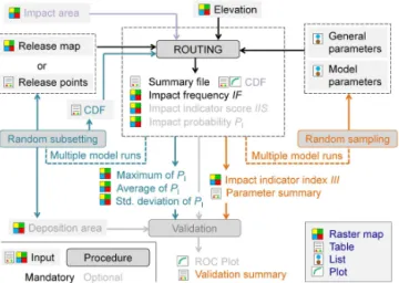
r.randomwalk was developed and tested with Ubuntu 12.04 LTS and is expected to also work on other UNIX systems. A simple user interface is available. However, the tool may be started more efficiently through command line parameters, enabling a straightforward batch-ing on the shell script level. This feature facilitates model testing, the combination with other GRASS GIS modules and the consideration of process chains (i.e., using the output of one analysis as the input for the next one). The logical framework is illustrated in Fig. 1, the key variables used in r.randomwalk are summarized in Table 1.
All tests (see Sect. 3) are performed on an Intel®
Core i7 975 with 3.33 GHz and 16 GB RAM (DDR3, PC3-1333 MHz), exploring a maximum of eight cores through hy-perthreading.
2.2 Random walk routing
Figure 1.Logical framework of r.randomwalk. Only those compo-nents covered in the present article are shown.
walk approaches are used for routing mass movements such as debris flows through elevation maps (DEMs), e.g. by Gamma (2000), Wichmann and Becht (2003), Mergili et al. (2012a), and Gruber and Mergili (2013). Such methods enable a certain degree of spreading of the movement by also considering other routing directions than the steepest de-scent. It avoids the concentration of flows – or any other types of mass movements – to linear features, which would not be realistic for debris flows, snow avalanches, or other types of mass movements. However, the routing is constrained or weighted by factors such as the slope or the perpetuation of the flow direction. An alternative to constrained random walk routing would consist in a multiple flow direction algorithm (Horton et al., 2013).
In the context of r.randomwalk, each random walk routes a hypothetic mass point from a release pixel through the DEM until a break criterion is reached (see Sect. 2.3). A large set of random walks is required for each mass point in order to achieve a satisfactory cover of the possible impact area. r.randomwalk is designed for
– one set of random walks for one mass movement, start-ing from a defined set of coordinates;
– multiple sets of random walks for one mass movement, one set starting from each pixel of the release area; – sets of random walks for multiple mass movements in
a study area (either starting from one set of coordinates per mass movement, or from all pixels defined as release areas);
– one set of random walks starting from each pixel in the study area.
Overlay rules for different random walks and sets of ran-dom walks are applied (see Sect. 2.4).
Figure 2.Control lengthLctrland segment lengthLseg.(a) Appli-cation ofLctrl to avoid sharp bending of the flow.(b)Smoothing of the flow path by introducing segments with maximum length of Lseg.
During the pixel-to-pixel routing procedure, turns of > 90◦
are not supported. Neighbour pixels are further considered invalid as target pixels in case they are out of the study area or conflict with at least one of the following limitations:
– In order to constrain upward movements, a user-defined maximum vertical run-up heightRmaxis introduced. It
takes the lowest elevation the random walk has passed through as reference.
– Certain types of mass flows (i.e., those with high vis-cosity) hardly change their flow direction sharply. The user-defined horizontal control distanceLctrldefines the
backward distance of each step over which the horizon-tal distance of motion has to increase (Fig. 2a).
The probabilityPpxof any other neighbour pixel px to
be-come the target pixel is
Ppx=
ppx
qxP=n
qx=1
pqx
, p=fdefβtanβ, (1)
wheren is the total number of valid neighbour pixels, and
β is the local slope between the current pixel and the con-sidered neighbour pixel.fdandfβ are weighting factors for the perpetuation of the flow direction and for the slope.fd
is governed by the input parameterd:fd=d2for the same
flow direction as the previous one,fd=d for a 45◦turn and
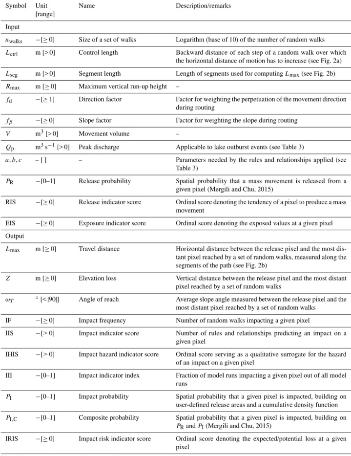
Table 1.Summary of the key variables used in r.randomwalk.
Symbol Unit Name Description/remarks [range]
Input
nwalks −[≥0] Size of a set of walks Logarithm (base of 10) of the number of random walks
Lctrl m [> 0] Control length Backward distance of each step of a random walk over which
the horizontal distance of motion has to increase (see Fig. 2a)
Lseg m [> 0] Segment length Length of segments used for computingLmax(see Fig. 2b)
Rmax m [≥0] Maximum vertical run-up height –
fd −[≥1] Direction factor Factor for weighting the perpetuation of the movement direction during routing
fβ −[≥0] Slope factor Factor for weighting the slope during routing
V m3[> 0] Movement volume –
Qp m3s−1[> 0] Peak discharge Applicable to lake outburst events (see Table 3)
a, b, c – [ ] – Parameters needed by the rules and relationships applied (see Table 3)
PR −[0–1] Release probability Spatial probability that a mass movement is released from a given pixel (Mergili and Chu, 2015)
RIS −[≥0] Release indicator score Ordinal score denoting the tendency of a pixel to produce a mass movement
EIS −[≥0] Exposure indicator score Ordinal score denoting the exposed values at a given pixel
Output
Lmax m [≥0] Travel distance Horizontal distance between the release pixel and the most dis-tant pixel reached by a set of random walks, measured along the segments of the path (see Fig. 2b)
Z m [≥0] Elevation loss Vertical distance between the release pixel and the most distant pixel reached by a set of random walks
ωT ◦[< |90|] Angle of reach Average slope angle measured between the release pixel and the most distant pixel reached by a set of random walks
IF −[≥0] Impact frequency Number of random walks impacting a given pixel
IIS −[≥0] Impact indicator score Number of rules and relationships predicting an impact on a given pixel
IHIS −[≥0] Impact hazard indicator score Ordinal score serving as a qualitative surrogate for the hazard of an impact on a given pixel
III −[0–1] Impact indicator index Fraction of model runs impacting a given pixel out of all model runs
PI −[0–1] Impact probability Spatial probability that a given pixel is impacted, building on user-defined release areas and a cumulative density function
PI,C −[0–1] Composite probability Spatial probability that a given pixel is impacted, building on PRandPI(Mergili and Chu, 2015)
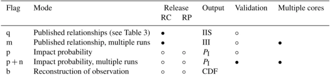
Table 2.Possibilities to define the break criteria. The flags provided through the command line or the user interface define the type of break criterion. RC is release coordinates (release from highest points of release areas), RP is release pixels (release from all pixels within release areas),•is relevant for most applications, and◦is relevant for some applications.
Flag Mode Release Output Validation Multiple cores RC RP
q Published relationships (see Table 3) • IIS ◦
m Published relationship, multiple runs • III ◦ • p Impact probability ◦ ◦ PI ◦
p+n Impact probability, multiple runs ◦ ◦ PI • • b Reconstruction of observation ◦ ◦ CDF
The break criteria for the random walks (see Sect. 2.3) are directly or indirectly related to the travel distanceLmaxi.e.,
the horizontal length between the release pixel and the ter-minal pixel measured along the flow path. Preliminary tests reveal that random walk routing through raster maps may re-sult in quite uneven flow paths (see Fig. 2b). Consequently, the distance calculated by summing up all the pixel-to-pixel distances may be significantly longer than the more relevant distance along the observed main flow paths. Employing the sums of the pixel-to-pixel distances would lead to an under-estimation of the angle of reach and, consequently, of the pre-dicted travel distances and impact areas. We approach this problem by dividing the flow paths into straight segments with a user-defined maximum length ofLseg. The travel
dis-tanceLmaxis defined as the sum of the length of all segments
(see Fig. 2b). Larger values ofLsegare expected to result in
shorter travel distances due to the more pronounced smooth-ing of the path.
2.3 Break criteria
Each random walk continues until at least one neighbour pixel is outside the study area, or until the user-defined break criterion is fulfilled. The break criteria are the key parameters for estimating the mass flow impact areas and can be defined in various ways (Table 2):
– The angle of reachωT or the maximum travel distance
Lmaxis computed from empirical–statistical rules or
re-lationships, based on the analysis of observed events (Table 3). They usually refer to the distance between the highest spot of the release area and the most dis-tant spot of the impact area along the flow path (the Fahrböschungaccording to Heim, 1932). Consequently, random walks using this type of break criterion have to start from the set of coordinates defining the highest point of the observed or expected mass movement. Al-ternatively, also a semi-deterministic model (Perla et al., 1980) can be used.
– Empirical–statistical relationships or the semi-deterministic model may be applied in a large number of parallel computations with randomized values of
the parameters a, b and c (see Fig. 1 and Table 3). This allows one to explore the effects of uncertainties in the relationships. Only one type of relationship is considered at once, and the output consists in a raster map of the impact indicator index III in the range 0–1, representing the fraction of tested parameter combi-nations predicting an impact on the pixel (i.e., where impact indicator score (IIS)=1). Further, the results of all model runs are stored in a way ready to be analysed with the parameter sensitivity and optimization tool AIMEC (Automated Indicator-based Model Evaluation and Comparison; Fischer, 2013).
– An impact probability raster mapPIin the range 0–1 is
computed from a user-defined sample of observed val-ues of tan(ωT), which is employed to build a cumulative density function (CDF). The CDF represents the prob-ability that the movement reaches the pixel associated with each value of tan(ωT). The sample of observed val-ues may be divided into one subset of mass movements for building the CDF, and another one for computingPI.
This ensures a clear separation between parameter op-timization and model validation (see Sect. 2.5). Parallel processing may be used to repeat the analysis for many random subsets in order to achieve a more robust result. – If an inventory of events is available, the observed im-pact areas may be back calculated by routing each ran-dom walk until it leaves the observed impact area of the corresponding mass movement. This mode can be used to explore the statistical distribution ofωT. The result-ing CDF can be used as input to estimatePI.
2.4 Overlay of random walk results
The overlay of individual random walks operates at two lev-els:
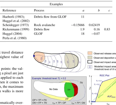
Table 3.Types of rules and relationships supported by r.randomwalk.ωT is angle of reach,Lmaxis travel distance,V is volume of motion, Zis elevation loss,Qpis peak discharge at release, andvTis velocity at termination.
ID Equation Examples
Reference Process a b c
1 ωT =a (2) Haeberli (1983); Debris flow from GLOF 11 Huggel et al. (2002)
2 log10tanωT =alog10V+b (3) Scheidegger (1973) Rock avalanche −0.15666 0.62419
3 Lmax=aVbZc (4) Rickenmann (1999) Debris flow 1.9 0.16 0.83 4 ωT =aQbp (5) Huggel (2004) GLOF 18 −0.07
5 vT=0 (6) Perla et al. (1980)
from the random walk with the shortest travel distance (i.e., the straightest flow path and the highest value of
ω) at the considered pixel.
2. Sets of random walks for different mass points: the val-ues of IF for all random walks impacting a pixel are just added up whilst the maximum of IIS is applied to each pixel. The issue gets more complex when it comes to
PI: depending on the specific application, the maximum
or the average out of all sets of random walks is more appropriate.
The resulting maps ofPIor IIS can be automatically
over-laid with a release probability (PR; result: composite
prob-ability PI,C; Mergili and Chu, 2015) or a release indicator
score (RIS; result: impact hazard indicator score – IHIS), and with an exposure indicator score (EIS) derived from the land cover (result: impact risk indicator score – IRIS; see Table 1). These steps are not further considered in this article and are therefore not shown in Fig. 1.
2.5 Validation
r.randomwalk includes three possibilities for validation of the model results. All three build on the availability of a raster map of the observed deposition area of the mass move-ment(s) under investigation. All parts of the observed impact areas outside of the observed deposition areas are set to no data (Fig. 3).
– For IIS, the true positive (TP), true negative (TN), false positive (FP), and false negative (FN) predictions are counted on the basis of pixels and put in relation. All pixels with IIS≥1 are considered as observed positives (OP); all pixels with IIS=0 are considered as observed negatives (ON).
– ROC (receiver operating characteristics) plots are pro-duced for III or PI: the true positive raterTP (TP/OP)
is plotted against the false positive raterFP(FP/ON) for
various levels of III orPI. The area under the curve
con-necting the resulting points, AUCROC, is used as an
indi-cator for the quality of the prediction (see Fig. 3). If the
Figure 3.Model validation with an ROC plot, relating the false pos-itive raterFPand the true positive raterTP. This way of validation
is suitable for predictor raster maps in the range 0–1, such as III or PI. It can also be used for binary predictor maps (0 or 1). In such a
case AUCROCis computed from two threshold levels only.
CDF forPIis derived from the same set of landslides,
r.randomwalk includes the option to randomly split the set of observed landslides into a set for parameter opti-mization, and one for validation. This is done for a user-defined number of times, exploiting multiple processors (see Sect. 2.3 and Fig. 1). It results in an ROC plot with multiple curves. Note that two ROC plots are produced: one of them builds on the original number of TN pix-els. For the other one, the number of ON pixels is set to 5 times the number of OP pixels. Whilst the num-ber of FP pixels remains unchanged, the numnum-ber of TN pixels is modified accordingly. This procedure aims at normalizing the ROC curves in order to enable a com-parison of the prediction qualities yielded for different study areas.
– If only one mass movement is considered, a longitudi-nal profile may be defined by a set of coordinates of the profile vertices. The observed and predicted (IIS≥1 orPI> 0) travel distances are measured and compared
3 Test cases and results
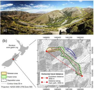
3.1 Acheron rock avalanche, New Zealand
3.1.1 Area description and model parameterization The Acheron rock avalanche in Canterbury, New Zealand (Fig. 4), was triggered approx. 1100 years BP (Smith et al., 2006). Within the present study, the release volume,
V =6.4 million m3, is approximated from the reconstruction
of the pre-failure topography and is lower than the value of
V =7.5 million m3estimated by Smith et al. (2006). We use
a 10 m resolution DEM derived by stereo-matching of aerial photographs. Impact, release and deposition areas are derived from field and imagery interpretation as well as from data published by Smith et al. (2006). All random walks start from the highest pixel of the release area.
We use this case study for demonstrating how to compute the impact indicator index III from an elevation map, the re-lease area, and the rere-lease volume. Before doing so, we have to analyse the influence of the pixel size and the parame-tersnwalks,Rmax,Lctrl,Lseg,fβ, andfdon the model result.
Preliminary tests have shown that r.randomwalk yields plau-sible results with the number of random walks:nwalks=104,
Rmax=10 m,Lctrl=1000 m,Lseg=100 m,fβ=5,fd=2, and a pixel size of 20 m. These values are taken as a basis to explore the sensitivity of the model results to the varia-tion of each parameter and the best fit of the parameters in terms of the travel distance, AUCROC, and the size of the
predicted impact area (Table 4).ωT =11.62◦, the angle of reach observed for the Acheron rock avalanche, is applied as the break criterion for all tests. Some of the tests are run in the back-calculation mode (flag b; see Tables 2 and 4).
III is computed by executing r.randomwalk 100 times, with the parameter values optimized according to Table 4. We explore an empirical–statistical relationship for ωT de-rived from a compilation of 127 case studies (Fig. 5). The offset of the equation (bin Eq. 4 and Fig. 5) is randomly
sam-pled between the lower and upper envelopes of the regres-sion. The quality of the prediction is evaluated using the ROC plot (see Figs. 1 and 3). Note that the Acheron rock avalanche (not included in the relationship developed in Fig. 5) is found close to the lower envelope, meaning that it was very mobile compared to most of the other events.
3.1.2 Results
Figure 6 summarizes the findings of the test s 1–3 (see Ta-ble 4). Test 1 leads to the expected result that the predicted impact area increases with the number of random walks. However, the predicted impact area is also a function of the pixel size: with larger pixels, less random walks are needed to cover an area of similar size than with smaller pixels. Fig-ure 6a further indicates that the possible impact area is not fully covered even at 105random walks: no substantial
flat-Figure 4. Acheron rock avalanche. (a) Panoramic view; photo: M. Mergili, 28 February 2015.(b)Location and geometry.
Figure 5.Empirical–statistical relationship relating the angle of reachωT to the volumeV of avalanching flows of rock or debris. The data are compiled from Scheidegger (1973), Legros (2002), Jib-son et al. (2006), Evans et al. (2009), Sosio et al. (2012), and Guo et al. (2014).
tening of the curves is observed. We conclude that (i) a very high value ofnwalks would be necessary to fully cover the
possible impact area, and (ii) this would lead to a substantial overestimation of the observed impact area.
On the other hand, the quality of the prediction in terms of AUCROCreaches a maximum at nwalks≈102(pixel size
40 m) or nwalks≈103 (pixel size 20 m), decreasing with
higher values of nwalks. At a pixel size of 10 m, AUCROC
reaches a constant level at nwalks≈104 (see Fig. 6b). We
Table 4.Tests of the parametersnwalks,Lctrl,Lseg,Rmax,fβ,fd, and the pixel size. Where ranges of values are given in bold, the model
is run with 100 random samples constrained by the minima and maxima indicated. Where values given in bold are separated by commas, in these cases exactly these values are tested.
Test nwalks Lctrl(m) Lseg(m) Rmax(m) fβ fd Pixel size (m)
11,3 100–106 1000 100 10 5 2 10, 20, 40
22 104 50, 1000 10–150 1000 5 2 10, 20, 40
31,2,3 104 50–10002 100 10002 5 2 10, 20, 402
1000–40001,3 101,3 201,3
41,3 104 1000 100 0–120 5 2 20
51,3 104 1000 100 10 0–10 2 20
61,3 104 1000 100 10 5 1–10 20
Test criteria:1impact area;2travel distanceLmax(flag b);3AUCROC.
Figure 6.Results of the tests 1–3 (number of test indicated in the yellow circle). Number of random walks plotted against(a)the impact area and(b)the area under the ROC curve.(c)Computed travel distanceLmaxas a function ofLseg(in the legend, the corresponding value
ofLctrlis given in parentheses).(d)ComputedLmaxas a function ofLctrl.
to an overestimation of the impact area rather than to a better prediction quality. Coarser pixel sizes allow one to achieve the same level of coverage and the same prediction quality at lower values ofnwalks. However, the pixel size has to be fine
enough to account for the main geometric characteristics of the process under investigation (see Sect. 4). All further tests are performed withnwalks=104.
Figure 6c illustrates that, atLctrl=1000 m, the travel
dis-tance computed within the observed impact area decreases with increasing values of Lseg (tests 2 and 3 in Table 4).
This pattern is well explained by Fig. 2b. At short segment lengths, the effects of flow paths frequently changing their direction are particularly evident for pixel sizes of 10 m and 20 m.Lmaxdrops below the observed value of 3550 m (see
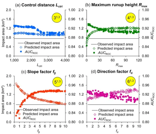
corre-Figure 7.Sensitivity of impact area and AUCROCto selected input parameters. The numbers of the corresponding tests (see Table 4) are indicated in the yellow circles.(a)Control distanceLctrl;(b)maximum run-up heightRmax;(c)slope factorfβ;(d)direction factorfd.
sponding to the Euclidean distance between the release point and the terminal point of the Acheron rock avalanche,Lmax
would also take a value of 3050 m. At Lctrl=50 m (only shown for a pixel size of 20 m), r.randomwalk tends to pre-dict too long travel distances, compared to the observation. This phenomenon occurs as flow directions are not well de-fined in the relatively plane deposition zone of the Acheron rock avalanche; therefore, flow paths may frequently change their direction or even go backwards or in a circular way if such a behaviour is not impeded by sufficiently high values ofLctrl(see Fig. 2a). Figure 6d indicates that this undesired
behaviour (visible in the area marked by the X in the gray circle) disappears atLctrl> 200 m.
On the other hand, the value of Lctrl should not be
cho-sen too high as this may negatively impact the model perfor-mance. In the case of the Acheron rock avalanche, a drop in AUCROC is observed between Lctrl≈2000 and Lctrl≈ 2500 m (Fig. 7a). This drop is explained by an increasing number of false negative pixels in those areas, which cannot be reached by the random walks due to the strict constraint of flow direction.
Within the tested ranges of parameter values, the quality of the prediction is highest at values ofRmax≈5–10 m (see
Fig. 7b) andfβ≥5 (see Fig. 7c), whilst it reaches it maxi-mum atfd≈2–3 (see Fig. 7d). The predicted impact area
in-creases with increasingRmaxandfdwhilst it decreases with
increasingfβ.
Figures 6 and 7 indicate that the initial values ofnwalks,
Lctrl, LsegRmax, fβ, fd, and the pixel size suggested in
Sect. 3.1.1 and Table 4 are within the optimum range of val-ues (see Sect. 4). Therefore, they are used for computing the impact indicator index for the Acheron rock avalanche (Fig. 8a). Concerning the break criteria, this can be classi-fied as a forward analysis. As expected from Fig. 5, where the Acheron rock avalanche falls in between the envelopes of the relationship employed, the upper part of the observed impact area displays a value of III=1, whilst the remaining part of the observed impact area displays values of 1 > III > 0, decreasing towards the terminus. As the event was compara-tively mobile within the context of the relationship used (see Sect. 3.1.1 and Fig. 5), the values of III are close to zero in the terminal area, and the area with III > 0 does not reach far beyond the observed terminus. Note that the maximum value of III is 0.8, meaning that 20 % of all model runs did not even start due to very high values ofωT yielded with the random-ized values ofb(see Fig. 5). Evaluation against the observed deposit yields a value of AUCROC=0.94 (see Fig. 8b). All
values of AUCROCshown in Figs. 6 and 7 and the ROC plot
Figure 8.Impact indicator score for the Acheron rock avalanche.
(a)Classified III map.(b)ROC plot, building on normalized ON
area (see Sect. 2.5).
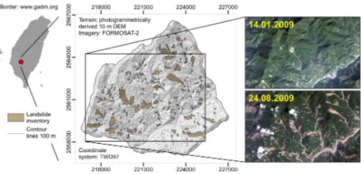
3.2 Kao Ping Watershed, Taiwan
3.2.1 Area description and model parameterization Between 7 and 9 August 2009, Typhoon Morakot struck Tai-wan and triggered enormous landslides, causing significant land cover change (Fig. 9). More than 22 000 landslides were recorded in southern Taiwan (Lin et al., 2011). One of the hot spots of mass wasting was the Kao Ping Watershed (Wu et al., 2011), where the extremely heavy rainfall (in total, more than 2000 mm depth and 90 h duration) triggered a catas-trophic landslide in the Hsiaolin Village (Kuo et al., 2013).
We consider a 61.5 km2subset of the Kao Ping Watershed for computing the landslide impact probabilityPI, based on
the observed landslide release areas. In all, 207 landslides are mapped in the shale, sandstone, and colluvium slopes (see Fig. 9). A 10 m DEM is used along with an inventory of the landslide impact areas. Release and deposition areas are ex-tracted from the inventory. We employ the values ofnwalks,
Rmax,fβ,fd,Lctrl,Lsegresulting from the optimization
pro-cedure for the Acheron rock avalanche (see Sect. 3.1.1), and a pixel size of 20 m.PIis computed as follows:
1. A set of random walks (nwalks=104) is started from
each release point (i.e., the highest pixel of each land-slide). Each random walk stops as soon as it would leave
Figure 9.Location, terrain and landslide inventory of the Kao Ping Watershed, Taiwan. Comparison of the satellite images illustrates the landslide-induced land cover changes associated with the Ty-phoon Morakot. The landslide inventory builds on the interpretation of the FORMOSAT-2 imagery.
the impact area of the same landslide (back calculation, flag b).
2. After completing all random walks for the study area, the statistical distribution ofωT is analysed. All land-slides with Lmax< 100 m are excluded. A fraction of
20 % out of all landslides (i.e., all values ofωT associ-ated with those landslides) is randomly selected and re-tained for validation. Using visual comparison, we have identified the log-normal distribution as the most suit-able type of distribution for this purpose. Consequently, the log-normal CDF stands for the probability that a moving mass point leaves the observed impact area at or below the associated threshold ofωT.
3. We perform a forward analysis ofPIby starting a set
of random walks (nwalks=104) from the release points
of the retained landslides, and assigning the cumulative density associated with the average angle of path to each pixel. The result is validated against the observed depo-sition zones of the retained landslides by means of an ROC plot.
4. Steps 2. and 3. are repeated for 100 randomly selected subsets (parallel processing is applied). The final map of
PIis generated by applying for each pixel the maximum
of the values yielded by all the model runs.
We refer to this work flow as test 1 and repeat the analysis with starting random walks not only from the release points but also from all the pixels within the observed release ar-eas (test 2). This means that the CDF is derived from a much larger sample of data than when considering only one point per landslide for starting random walks. We exclude all sets of random walks yielding Lmax< 100 m, use a log-normal
3.2.2 Results
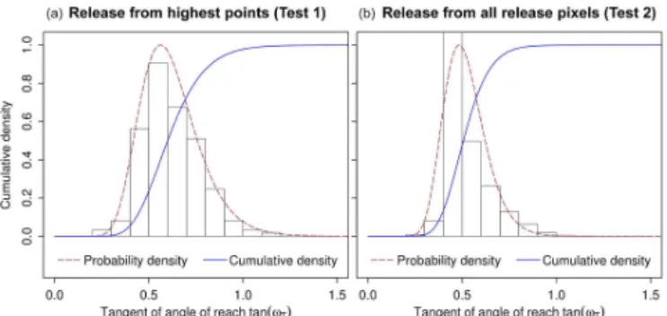
Starting sets of 104 random walks from the highest points
of all landslides (test 1) results in a range of values of 16.0≤ωT ≤43.5◦, an average of 30.4◦, and a standard de-viation of 5.2◦ (derived from n=132 landslides,
exclud-ing those with Lmax< 100 m). Repeating the analysis with
104 random walks started from each pixel within the land-slide release areas (test 2), we observe a range of values 16.4≤ωT ≤44.1◦, an average of 26.9◦, and a standard devi-ation of 4.8◦(n=1563). Figure 10 illustrates the histograms,
probability density, and cumulative density functions derived from both analyses. Even though the ranges of values are similar in both tests, test 1 yields (i) a higher average ofωT and (ii) a broader range of values than test 2; (i) is explained by the fact that those random walks starting from lower parts of the release areas are expected to leave the observed impact area at lower values ofωT; (ii) is most likely the consequence of a number of rather small landslides with high or low val-ues of ωT strongly reflected in the statistics. Such outliers are less prominent in the statistics of test 2 due to the much higher number of cases, most of them related to the larger landslides.
Each of the impact probabilities shown in Fig. 11 repre-sents the overlay of 100 analyses where random sets of 80 % of the landslides are used for deriving the CDF and the re-maining 20 % are used for computing the impact probabil-ities. The maps illustrate the maximum values ofPIout of
the overlay of the 100 results. Each of the results is derived using a slightly different CDF. Both tests yield largely simi-lar patterns ofPI. We note that (i) test 2 predicts larger
im-pact areas and higher values ofPIthan test 1, and (ii) some
random walks take the wrong direction in test 2 (indicated by “1” in the yellow circle in Fig. 11b), a phenomenon not observed for test 1; (i) is explained by the higher number – and the broader distribution – of release pixels in test 2, compared to test 1. The reason for (ii) is that random walks starting from the highest point of an observed landslide are forced to flow into the observed landslide area (test 1), a con-straint not applicable when starting random walks from each release pixel (test 2). In this case it happens that pixels lo-cated at or near a crest produce random walks in both di-rections. In test 1, the computational time amounted to 63 s for deriving the CDF and 8613 s for calculatingPI. In test 2,
these times increased to 1719 and 9752 s, respectively. The relatively slight increase with regard to PI results from the
reduced value ofnwalksin test 2.
The prediction quality is tested for each of the 100 model runs for the two tests, producing sets of 100 ROC curves (Fig. 12). AUCROC=0.917±0.038 for test 1 and
0.920±0.029 for test 2, both computed with the original number of TN pixels (see Sect. 2.5).
In contrast, the procedures demonstrated in the two tests vary strongly in their scope of applicability. We have
demon-Figure 10.Histograms, probability densities, and cumulative den-sities ofωT of mass movements in the test area in the Kao Ping Watershed.(a)Result for a set of 104random walks started from the highest point of each landslide (test 1).(b)Result for a set of 104random walks started from each pixel within the release areas of all landslides (test 2).
strated the methodologies by back calculating observed land-slides. As soon as this is done, one may go one step further:
– The methodology shown in test 1 can be employed to make forward predictions for defined expected future landslides, given that a sufficient set of observed land-slides of similar behaviour is available to derive the CDF.
– The methodology demonstrated in test 2 can be used in combination with maps of landslide release probability to explore the composite probability of a landslide im-pact (see Sects. 2.4 and 4).
In either case the statistics (see Fig. 10) have to be derived with the same type of approach later used for producing the
PImap.
3.3 Gunt Valley, Tajikistan
3.3.1 Area description and model parameterization As most mountain areas worldwide, the Pamir of Tajikistan experiences a significant retreat of the glaciers. One of the consequences thereof consists in the formation and growth of lakes, some of which are subject to glacial lake outburst floods (GLOFs), which may evolve into destructive debris flows (Mergili and Schneider, 2011; Mergili et al., 2013; Gruber and Mergili, 2013). No records of historic GLOFs in the test area are known to the authors. However, in Au-gust 2002 a GLOF in the nearby Shakhdara Valley evolved into a debris flow, which destroyed the village of Dasht, claiming dozens of lives (Mergili et al., 2011).
Figure 11.Impact probability in the range 0–1.(a)Result of test 1 (random walks starting from the highest point of each landslide; cumulative density according to Fig. 10a).(b)Result of test 2 (random walks starting from all release pixels; cumulative density according to Fig. 10b).
Figure 12.ROC plots illustrating the prediction quality of(a)test 1 and(b)test 2, using the original number of TN pixels (see Sect. 2.5).
We compute IIS with regard to GLOFs for a 2106 km2 study area in the Gunt Valley (Fig. 13). The analysis builds on the ASTER GDEM (Advanced Spaceborne Thermal Emis-sion and Reflection Radiometer – Global Digital Elevation Model) V2 and the coordinates and characteristics (estimates ofV andQp) of 113 lakes in the area (Gruber and Mergili,
2013).
A set of random walks (nwalks=104) is routed from the outlet of each lake through the DEM. Six break criteria are combined to compute IIS, partly following Gruber and Mergili (2013). The relationships and rules employed as break criteria are summarized in Table 5. Rule 1 is applied with ωT =11◦ (test 1 – according to Haeberli, 1983 and Huggel et al., 2003, 2004a, b for debris flows from glacier-or mglacier-oraine-dammed lakes, and Zimmermann et al., 1997 fglacier-or coarse- and medium-grained debris flows) and withωT =7◦ (test 2 – Zimmermann et al., 1997 for fine-grained debris flows). All other rules and relationships are used for both tests. For each pixel, IIS consists in the number of relation-ships or rules predicting an impact (i.e., IIS takes values in the range 0–6).
Rmax,Lctrl,Lseg,fβ, andfdare set to the optimum values
found for the Acheron rock avalanche, the pixel size is set to 60 m.
3.3.2 Results
Figure 14 illustrates the possible impact areas of GLOFs in the Gunt Valley study area according to the relationships listed in Table 5.
Figure 14a shows the impact indicator score IIS i.e., the number of relationships predicting an impact, resulting from test 1 (rule 1 applied withωT =11◦). Except for one promi-nent exception, IIS > 3 (possible debris flow impact) only for the largely uninhabited upper portions of the tributaries to the Gunt Valley. In contrast, a possible flood impact (1≤IIS≤3) is predicted for much of the main valley. test 2 (rule 1 applied withωT =7◦) predicts a possible debris flow impact also for part of the main valleys (see Fig. 14b). The IF (per cent of random walks impacting each pixel) for test 1 is shown in Fig. 14c for a subsection of the test area, classified by quan-tiles. IF is strongly governed by the width of the movement, i.e. by the local topography, and may serve as a surrogate for the expected depth rather than as for the probability of an impact.
Figure 13.The test area in the Gunt Valley, Tajikistan.(a)Location, topography, glaciers and lakes.(b)Proglacial lake in the upper Varshedz-dara Valley; photo: M. Mergili, 18 August 2011.
Table 5.Empirical–statistical relationships and simple rules used for computing the IIS of GLOFs in the Gunt Valley (see Table 3).
IDtest Relationship Reference Process
11 ωT =11◦ Haeberli (1983); Zimmermann et al. (1997);
Flood or debris flow Huggel et al. (2003, 2004a, b)
12 ωT =7◦ Zimmermann et al. (1997) 21,2 ω
T =18Q−0p .07 Huggel (2004)
31,2 L
max=1.9V0.16Z0.83 Rickenmann (1999)3 41,2 ω
T =6◦
Flood 51,2 ω
T =4◦ 61,2 ω
T =2◦ Haeberli (1983); Huggel et al. (2004a)
1,2ID(s) of test(s) where the rule or relationship is applied.3A bulking factor of 5 is applied toV(modified after Iverson, 1997).
The robustness and appropriateness of the rules and re-lationships for low-frequency events, such as GLOFs (see Table 5), is questionable. The rules building on a unique value ofωT overpredict the possible impact areas for those lakes where not enough water is available to produce a flood in downstream valleys. Applying the rules and rela-tionships for debris flows implies a blind assumption that enough entrainable sediment is available to produce a de-bris flow. WhilstωT ≥11◦is considered the worst case for debris flows of GLOFs from glacier- or moraine-dammed lakes in the European Alps according to Haeberli (1983) and Huggel et al. (2002),ωT =9.3◦was measured for the 2002 Dasht Event, the only well-documented GLOF near the test area (Mergili et al., 2011). Also the relationship proposed by Rickenmann (1999) severely underestimates the travel dis-tance of this event, even when massive bulking is assumed. ApplyingωT =7◦as given by Zimmermann et al. (1997) for fine-grained debris flows might be more suitable as worst-case assumption for debris flows from GLOFs in the Pamir, even though this threshold leads to very conservative predic-tions.
We have measured computational times of 1520 s for test 1 and 1556 s for test 2.
4 Discussion
Re-Figure 14.Possible GLOF impact areas in the Gunt Valley, Tajikistan.(a)Impact indicator score derived with test 1.(b)Impact indicator
score derived with test 2.(c)Impact frequency derived with test 1, classified by quantiles.
lationships for less frequent types of processes are less ro-bust as it was illustrated for GLOFs (Haeberli, 1983; Zim-mermann et al.; 1997; Huggel et al., 2002; Huggel, 2004; see Sect. 3.3.2). In such cases we recommend to compute impact indicator scores building on more than one model, as shown by Gruber and Mergili (2013) and in the present work. Impact indicator indices and scores are mainly useful for anticipating the possible impact area of expected single events (see Sect. 3.1.2), or for application at broader scales (see Sect. 3.3.2).
The impact probability is useful for predicting possible im-pact areas of mass movements in areas where many events are documented, but the volumes of possible future events are not known. Whilst in the present paper it was demon-strated how to compute impact probabilities related to ob-served release areas, r.randomwalk also includes the option to combine the impact probability with the release probabil-ityPR(see Table 1). Landslide release probability
(suscep-tibility) maps are often produced from a landslide inventory and a set of environmental layers (e.g., Guzzetti, 2006). Start-ing random walks from each sStart-ingle pixel of a study area, and combining the release probability of this pixel with the im-pact probability allows one to produce a composite probabil-ityPI,Cmap. Doing this is non-trivial and requires specific
strategies. It is therefore covered in a separate article (Mergili and Chu, 2015). Gruber and Mergili (2013) have combined release and impact indicator scores for various types of high-mountain hazards, and overlaid the results with a land cover data set to produce a risk indicator score.
The sensitivity of r.randomwalk to variations of the param-etersnwalks,Rmax,fβ,fd,Lctrl,Lseg(see Sect. 2.2) and the
pixel size were tested for the Acheron rock avalanche. Even though the optimized values are applied also to the other cases in the present work, this issue requires further inves-tigation, also with regard to the scale of the processes. This is particularly true for the pixel size, which has to be fine enough not to lose the geometrical characteristics governing the motion (Blahut et al., 2010). Furthermore, coarser pix-els and a larger number of random walks make results more conservative.Rmax,fβ, andfdcontrol the degree of lateral
spreading and therefore influence the conservativeness of the results. In the future we plan to compare the performance of r.randomwalk to software tools using multiple flow direc-tion algorithms (e.g., Flow-R; Horton et al., 2013) in terms of computational times and prediction success.
Overestimating the travel distance at a certain pixel is avoided by choosing sufficiently high values of Lseg (see
Fig. 6c). Shorter travel distances at a certain pixel are as-sociated with higher values ofω and, consequently, larger predicted impact areas, i.e. more conservative results that are desirable for many applications. The values of Rmax
lead-ing to the best prediction quality are considerably lower than run-up height observed for the Acheron rock avalanche. This phenomenon is explained by the facts that (i) the observed maximum run-up height refers to a limited area, whilst r.randomwalk applies the run-up height defined byRmaxin
We have demonstrated how to estimate the prediction quality of III andPI maps. Where sufficient reference data
are available to prove the validity of the model, the results may be applied for hazard zoning. Where data are not avail-able, the outcomes of r.randomwalk are suitable for broad-scale overviews of possibly affected areas, which have to be considered as rough indicators only. A suitable level of spa-tial aggregation may be necessary in such cases (Gruber and Mergili, 2013).
r.randomwalk includes a break criterion building on the two-parameter friction model of Perla et al. (1980) (see Sect. 1 and Table 3), which can be used to compute flow velocities (e.g., Wichmann and Becht, 2013; Mergili et al., 2012a; Horton et al., 2013). Evaluating this functionality has to build on (i) specific strategies for the sensitivity analy-sis and optimization of multiple parameters and (ii) a sound comparison with the outcome of physically based models. This effort will be presented in a separate article (Krenn et al., 2015). Further, the parameter sensitivity and optimiza-tion code AIMEC (Fischer, 2013) can be directly coupled to r.randomwalk.
5 Conclusions
We have introduced the open-source GIS tool r.randomwalk, designed for conceptual modelling of the propagation of mass movements. r.randomwalk offers built-in functions for considering uncertainties and for validation. Employing a set of three contrasting test areas, we have demonstrated (i) the possibility to combine results yielded with various break cri-teria into one impact indicator score; (ii) the option to explore multiple computational cores for combining the results ob-tained with many randomized parameter combinations into an impact indicator index; (iii) the possibility to back calcu-late the CDF of the angles of reach of observed landslides, and to use this CDF to make forward predictions of the im-pact probability; and (iv) integrated functions for the valida-tion and visualizavalida-tion of the results. This includes strategies to properly separate the data sets for parameter optimization and model validation.
We have further shown that controls for smoothing of the flow path and the avoidance of circular flows have to be intro-duced to avoid underestimating travel distances and impact areas. The number of random walks executed for each mass point and the pixel size influence the level of conservative-ness of the results rather than the quality of the prediction. The scope of applicability of r.randomwalk strongly depends on the availability of robust break criteria and on the avail-ability of reference data for evaluation.
Code availability
The model codes, a user manual, the scripts used for starting the tests presented in Sect. 3 and some of the test data are available at http://www.mergili.at/randomwalk.html.
Acknowledgements. The work was conducted as part of the international cooperation project “A GIS simulation model for avalanche and debris flows” funded by the Austrian Science Fund (FWF) and the German Research Foundation (DFG). Further, the support of Massimiliano Alvioli, Matthias Benedikt, Yi-Chin Chen, Ivan Marchesini, and Tim Davies is acknowledged.
Edited by: T. Poulet
References
Blahut, J., Horton, P., Sterlacchini, S., and Jaboyedoff, M.: De-bris flow hazard modelling on medium scale: Valtellina di Tirano, Italy, Nat. Hazards Earth Syst. Sci., 10, 2379–2390, doi:10.5194/nhess-10-2379-2010, 2010.
Burton, A. and Bathurst, J. C.: Physically based modelling of shal-low landslide sediment yield at a catchment scale, Environ. Geol., 35, 89–99, 1998.
Christen, M., Bartelt, P., and Kowalski, J.: Back calculation of the In den Arelen avalanche with RAMMS: interpretation of model results, Ann. Glaciol., 51, 161–168, 2010a.
Christen, M., Kowalski, J., and Bartelt, B.: RAMMS: Numerical simulation of dense snow avalanches in three-dimensional ter-rain, Cold Reg. Sci. Technol., 63, 1–14, 2010b.
Corominas, J., Copons, R., Vilaplana, J. M., Altamir, J., and Amigó, J.: Integrated Landslide Susceptibility Analysis and Hazard As-sessment in the Principality of Andorra, Nat. Hazards, 30, 421– 435, 2003.
Evans, S. G., Roberts, N. J., Ischuk, A., Delaney, K. B., Morozova, G. S., and Tutubalina, O.: Landslides triggered by the 1949 Khait earthquake, Tajikistan, and associated loss of life, Eng. Geol., 109, 195–212, 2009.
Fischer, J.-T.: A novel approach to evaluate and compare computa-tional snow avalanche simulation, Nat. Hazards Earth Syst. Sci., 13, 1655–1667, doi:10.5194/nhess-13-1655-2013, 2013. Gamma, P.: Dfwalk – Murgang-Simulationsmodell zur
Gefahren-zonierung, Geographica Bernensia, G66, ISBN 3-906151-53-0, University of Bern, Switzerland, 144 pp., 2000.
GRASS Development Team: Geographic Resources Analysis Sup-port System (GRASS) Software, Version 7.0. Open Source Geospatial Foundation, availble at: http://grass.osgeo.org, last access: 27 July 2015.
Gruber, F. E. and Mergili, M.: Regional-scale analysis of high-mountain multi-hazard and risk indicators in the Pamir (Tajik-istan) with GRASS GIS, Nat. Hazards Earth Syst. Sci., 13, 2779– 2796, doi:10.5194/nhess-13-2779-2013, 2013.
Guo, D., Hamada, M., He, C., Wang, Y., and Zou, Y.: An empir-ical model for landslide travel distance prediction in Wenchuan earthquake area, Landslides, 11, 281–291, 2014.
Heim, A.: Bergsturz und Menschenleben, Fretz und Wasmuth, Zürich, 1932.
Hergarten, S. and Robl, J.: Modelling rapid mass movements using the shallow water equations in Cartesian coordinates, Nat. Haz-ards Earth Syst. Sci., 15, 671–685, doi:10.5194/nhess-15-671-2015, 2015.
Horton, P., Jaboyedoff, M., Rudaz, B., and Zimmermann, M.: Flow-R, a model for susceptibility mapping of debris flows and other gravitational hazards at a regional scale, Nat. Hazards Earth Syst. Sci., 13, 869–885, doi:10.5194/nhess-13-869-2013, 2013. Huggel, C.: Assessment of Glacial Hazards based on Remote
Sens-ing and GIS ModelSens-ing, Dissertation at the University of Zurich, Schriftenreihe Physische Geographie Glaziologie und Geomor-phodynamik, Zurich, Switzerland, 2004.
Huggel, C., Kääb, A., Haeberli, W., Teysseire, P., and Paul, F.: Re-mote sensing based assessment of hazards from glacier lake out-bursts: a case study in the Swiss Alps, Can. Geotech. J., 39, 316– 330, 2002.
Huggel, C., Kääb, A., Haeberli, W., and Krummenacher, B.: Regional-scale GIS-models for assessment of hazards from glacier lake outbursts: evaluation and application in the Swiss Alps, Nat. Hazards Earth Syst. Sci., 3, 647–662, doi:10.5194/nhess-3-647-2003, 2003.
Huggel, C., Haeberli, W., Kääb, A., Bieri, D., and Richardson, S.: Assessment procedures for glacial hazards in the Swiss Alps, Can. Geotech. J., 41, 1068–1083, 2004a.
Huggel, C., Kääb, A., and Salzmann, N.: GIS-based modeling of glacial hazards and their interactions using Landsat-TM and IKONOS imagery, Norsk Geogr. Tidsskr., 58, 761–773, 2004b. Hungr, O., Corominas, J., and Eberhardt, E.: State of the Art
pa-per: Estimating landslide motion mechanism, travel distance and velocity, in: Landslide Risk Management, edited by: Hungr, O., Fell, R., Couture, R., Eberhardt, E., Proceedings of the Interna-tional Conference on Landslide Risk Management, Vancouver, Canada, 31 May–3 June 2005, 129–158, 2005.
Iverson, R. M.: The physics of debris flows, Rev. Geophys., 35, 245–296, 1997.
Jibson, R. W., Harp, E. L., Schulz, W., and Keefer, D. K.: Large rock avalanches triggered by the M 7.9 Denali Fault, Alaska, earth-quake of 3 November 2002, Eng. Geol., 83, 144–160, 2006. Krenn, J., Mergili, M., Fischer, J.-T., Davies, T., Frattini, P., and
Pudasaini, S. P.: Optimizing the parameterization of mass flow models, manuscript submitted to the Proceedings of the 12th In-ternational Symposium on Landslides, Naples, Italy, 12–19 June 2016, 2015.
Kuo, Y. S., Tsai, Y. J., Chen, Y. S., Shieh, C. L., Miyamoto, K., and Itoh, T.: Movement of deep-seated rainfall-induced landslide at Hsiaolin Village during Typhoon Morakot, Landslides, 10, 191– 202, 2013.
Legros, F.: The mobility of long-runout landslides, Eng. Geol., 63, 301–331, 2002.
Lied, K. and Bakkehøi, S.: Empirical calculations of snow-avalanche run-out distance based on topographic parameters, J. Glaciol., 26, 165–177, 1980.
Lin, C. W., Chang, W. S., Liu, S. H., Tsai, T. T., Lee, S. P., Tsang, Y. C., Shieh, C. J., and Tseng, C. M.: Landslides triggered by the 7 August 2009 Typhoon Morakot in southern Taiwan, Eng. Geol., 123, 3–12, 2011.
McClung, D. M. and Lied, K.: Statistical and geometrical definition of snow avalanche runout, Cold Reg. Sci. Tech., 13, 107–119, 1987.
McDougall, S. and Hungr, O.: A Model for the Analysis of Rapid Landslide Motion across Three-Dimensional Terrain, Canadian Geotech. J., 41, 1084–1097, 2004.
McDougall, S. and Hungr, O.: Dynamic modeling of entrainment in rapid landslides, Canadian Geotech. J., 42, 1437–1448, 2005. Mergili, M. and Chu, H.-J.: Integrated statistical modelling of
spa-tial landslide probability, Nat. Hazards Earth Syst. Sci. Discuss., 3, 5677–5715, doi:10.5194/nhessd-3-5677-2015, 2015. Mergili, M. and Schneider, J. F.: Regional-scale analysis of lake
outburst hazards in the southwestern Pamir, Tajikistan, based on remote sensing and GIS, Nat. Hazards Earth Syst. Sci., 11, 1447– 1462, doi:10.5194/nhess-11-1447-2011, 2011.
Mergili, M., Schneider, D., Worni, R., and Schneider, J. F.: Glacial lake outburst floods in the Pamir of Tajikistan: challenges in prediction and modelling, in: Proceedings of the 5th Interna-tional Conference on Debris-Flow Hazards Mitigation: Mechan-ics, Prediction and Assessment, edited by: Genevois, R., Hamil-ton, D. L., and Prestininzi, A., Padua, Italy, 14–17 June 2011, Italian J. Eng. Geol. Environ. – Book, 973–982, 2011.
Mergili, M., Fellin, W., Moreiras, S. M., and Stötter, J.: Simulation of debris flows in the Central Andes based on Open Source GIS: Possibilities, limitations, and parameter sensitivity, Nat. Hazards, 61, 1051–1081, 2012a.
Mergili, M., Schratz, K., Ostermann, A., and Fellin, W.: Physically-based modelling of granular flows with Open Source GIS, Nat. Hazards Earth Syst. Sci., 12, 187–200, doi:10.5194/nhess-12-187-2012, 2012b.
Mergili, M., Müller, J. P., and Schneider, J. F.: Spatio-temporal de-velopment of high-mountain lakes in the headwaters of the Amu Darya river (Central Asia), Global Planet. Change, 107, 13–24, 2013.
Mergili, M., Marchesini, I., Alvioli, M., Metz, M., Schneider-Muntau, B., Rossi, M., and Guzzetti, F.: A strategy for GIS-based 3-D slope stability modelling over large areas, Geosci. Model Dev., 7, 2969–2982, doi:10.5194/gmd-7-2969-2014, 2014. Mergili, M., Fischer, J.-T., Fellin, W., Ostermann, A., and
Puda-saini, S. P.: An advanced open source computational frame-work for the GIS-based simulation of two-phase mass flows and process chains, EGU General Assembly, Vienna, Austria, 12– 17 April 2015, Geophys. Res. Abs., 17, 2015.
Neteler, M. and Mitasova, H.: Open source GIS: a GRASS GIS ap-proach, Springer, New York, USA, 2007.
Pearson, K: The Problem of the Random Walk, Nature, 72, 294, 318, 342, 1905.
Perla, R., Cheng, T. T., and McClung, D. M.: A Two-Parameter Model of Snow Avalanche Motion, J. Glaciol., 26, 197–207, 1980.
Pitman, E. B. and Le, L.: A two-fluid model for avalanche and de-bris flows, Philos. T. R. Soc. A, 363, 1573–1601, 2005. Pudasaini, S. P.: A general two-phase debris flow model, J.
Geo-phys. Res., 117, F03010, doi:10.1029/2011JF002186, 2012. Pudasaini, S. P. and Hutter, K.: Avalanche Dynamics: Dynamics of
R Core Team: R: A Language and Environment for Statistical Com-puting, R Foundation for Statistical ComCom-puting, Vienna, Austria, available at: http://www.R-project.org, last access: 27 July 2015. Rickenmann, D.: Empirical Relationships for Debris Flows, Nat.
Hazards, 19, 47–77, 1999.
Savage, S. B. and Hutter, K.: The motion of a finite mass of granular material down a rough incline, J. Fluid Mech., 199, 177–215, 1989.
Scheidegger, A. E.: On the Prediction of the Reach and Velocity of Catastrophic Landslides, Rock Mech., 5, 231–236, 1973. Scheidl, C. and Rickenmann, D.: Empirical prediction of
debris-flow mobility and deposition on fans, Earth Surf. Proc. Land-forms, 35, 157–173, 2010.
Smith, G. M., Davies, T. R., McSaveney, M. J., and Bell, D. H.: The Acheron rock avalanche, Canterbury, New Zealand – morphol-ogy and dynamics, Landslides, 3, 62–72, 2006.
Sosio, R., Crosta, G. B., Chen J. H., and Hungr, O.: Modelling rock avalanche propagation onto glaciers, Quat. Sci. Rev., 47, 23–40, 2012.
Takahashi, T., Nakagawa, H., Harada, T., and Yamashiki, Y.: Rout-ing debris flows with particle segregation, J. Hydraul. Res., 118, 1490–1507, 1992.
Vandre, B. C.: Rudd Creek debris flow, in: Delineation of landslide, flash flood and debris flow hazards in Utah, edited by: Bowles, D. S., Utah Water Research Laboratory, Logan, Utah, USA, 117– 131, 1985.
Voellmy, A.: Über die Zerstörungskraft von Lawinen, Schweiz-erische Bauzeitung, 73, 159–162, 212–217, 246–249, 280–285, 1955.
Wichmann, V. and Becht, M.: Modelling of Geomorphic Pro-cesses in an Alpine Catchment, in: Proceedings of the 7th In-ternational Conference on GeoComputation, 8–10 September 2003, University of Southampton, UK, availabe at: http://www. geocomputation.org/2003/Papers/Wichmann_Paper.pdf (last ac-cess: 11 December 2015), 2003.
Wu, C. H., Chen, S. C., and Chou, H. T.: Geomorphologic charac-teristics of catastrophic landslides during typhoon Morakot in the Kaoping Watershed, Taiwan, Eng. Geol., 123, 13–21, 2011. Zimmermann, M., Mani, P., and Gamma, P.: Murganggefahr und