www.hydrol-earth-syst-sci.net/20/3673/2016/ doi:10.5194/hess-20-3673-2016
© Author(s) 2016. CC Attribution 3.0 License.
Shift of annual water balance in the Budyko space for catchments
with groundwater-dependent evapotranspiration
Xu-Sheng Wang1and Yangxiao Zhou2
1Ministry of Education Key Laboratory of Groundwater Circulation and Evolution, China University of Geosciences, Beijing 100083, China
2UNESCO-IHE Institute for Water Education, Delft, the Netherlands
Correspondence to:Xu-Sheng Wang (wxsh@cugb.edu.cn)
Received: 8 October 2015 – Published in Hydrol. Earth Syst. Sci. Discuss.: 4 November 2015 Revised: 28 July 2016 – Accepted: 2 August 2016 – Published: 8 September 2016
Abstract.The Budyko framework represents the general re-lationship between the evapotranspiration ratio (F) and the aridity index (ϕ) for the mean annual steady-state water balance at the catchment scale. It is interesting to investi-gate whether this standard F−ϕ space can also be applied to capture the shift of annual water balance in catchments with varying dryness. Previous studies have made significant progress in incorporating the storage effect into the Budyko framework for the non-steady conditions, whereas the role of groundwater-dependent evapotranspiration was not inves-tigated. This study investigates how groundwater-dependent evapotranspiration causes the shift of the annual water bal-ance in the standard Budyko space. A widely used monthly hydrological model, the ABCD model, is modified to in-corporate groundwater-dependent evapotranspiration into the zone with a shallow water table and delayed groundwater recharge into the zone with a deep water table. This model is applied in six catchments in the Erdos Plateau, China, to estimate the actual annual evapotranspiration. Results show that the variations in the annualF value with the aridity in-dex do not satisfy the standard Budyko formulas. The shift of the annual water balance in the standard Budyko space is a combination of the Budyko-type response in the deep groundwater zone and the quasi-energy limited condition in the shallow groundwater zone. Excess evapotranspiration (F> 1) could occur in dry years, which is contributed by the significant supply of groundwater for evapotranspiration. Use of groundwater for irrigation can increase the frequency of theF> 1 cases.
1 Introduction
Estimating catchment water balance is one of the funda-mental tasks in hydrology. Efforts have long been devoted to construct the physical, empirical, and statistical mod-els to explain the general relationship between precipitation (P), runoff (Q), potential evapotranspiration (E0)and ac-tual evapotranspiration (E) in terms of mean annual fluxes at the catchment scale (Budyko, 1948, 1958, 1974; Mezent-sev, 1955; Fu, 1981; Porporato et al., 2004; Yang et al., 2008; Gerrits et al., 2009). A simple and highly intuitive approach widely used for estimatingEat the mean annual steady state is the Budyko framework, in which the mean annual evapo-transpiration ratio (E/P) was presumed to be a function of the climatic dryness:
E
P =F
E0
P
=F (ϕ), (1)
where ϕ is the aridity index defined as E0/P, and F(ϕ) is an empirical function that relates E/P to ϕ based on general water-energy balance. The proposed formula by Budyko (1958, 1974) was
F (ϕ)=pϕ[1−exp(−ϕ)]tanh(1/ϕ), (2)
which indicates a nonlinear relation betweenF andϕ. This
F−ϕcurve has been called the Budyko curve (Zhang et al., 2004; Roderick and Farquhar, 2011) and theF−ϕspace was called the Budyko space (Renner et al., 2012).
properties such as soils and vegetation (Mezentsev, 1955; Fu, 1981; Zhang et al., 2001). For example, Fu’s equation (Fu, 1981) was derived following the idea of Mezentsev (1955), which can be expressed as follows:
F (ϕ, w)=1+ϕ−(1+ϕw)1/w, (3)
where w is a parameter representing the catchment condi-tions. F increases with w, leading to reduced Q/P as w
grows (Fu, 1981). Fu’s equation has been widely used in the last decade (Zhang et al., 2004, 2008; Yang et al., 2006, 2007; Greve et al., 2015). Donohue et al. (2007) highlighted the role of vegetation dynamics in the application of the Budyko framework. Wang and Tang (2014) also developed a one-parameter Budyko model based on the proportionality hy-pothesis and revealed a complex relationship between the catchment-specific parameter and the remote sensing vege-tation index. These modified formulas suggested a group of Budyko curves instead of the single original Budyko curve, in which a curve represents a specific type of catchments with similar features controlling the mean annual water bal-ance. Nevertheless, Gentine et al. (2012) argued that the orig-inal Budyko curve reflects the interdependence among veg-etation, soil and climate, and could be applied as a strong constraint on land-surface parameterizations.
The Budyko hypothesis has been directly used to ana-lyze the interannual change in water balance in catchments (Koster and Suarez, 1999; Arora, 2002; Zhang et al., 2008; Potter and Zhang, 2009), ignoring the change in storage (1S) under the assumption of steady-state water balance. One can plot annually the estimated F data in the standard Budyko space to check whether the standard Budyko curves are suf-ficient or not to represent the interannual variability of evap-otranspiration with the varying dryness. In this way, Potter and Zhang (2009) found that the Budyko framework is gen-erally applicable for the catchments in Australia and that the optimal Budyko curve of the annualF−ϕdata is highly de-pendent on the seasonal variations in rainfall. However, this approach should be carefully used when the annualF value is approximated by the annual (P−Q)/P value. Wang et al. (2009) and Istanbulluoglu et al. (2012) reported that the annual data of (P−Q)/P in some basins are negatively re-lated to the aridity index, exhibiting an inverse relation in comparison with the standard Budyko curves. According to long-term groundwater observations in the North Loup River basin, Nebraska, USA, Istanbulluoglu et al. (2012) demon-strated that the annualF data estimated by (P−Q−1G)/P
basically follow the Budyko hypothesis, where 1G is the change in groundwater storage. However, in some other stud-ies, an unexpected high evapotranspiration ratio (F> 1) was observed (Cheng et al., 2011; Wang, 2012; Chen et al., 2013). Among the 12 watersheds investigated by Wang (2012), half of them had such highF values in 2 or more drought years. The physical base of the phenomena is the significant con-tribution of storage in dry periods by which the high level of evapotranspiration is maintained. Although some of the
cases were triggered by extracting groundwater for irrigation in farmlands (Cheng et al., 2011; Wang, 2012), it could oc-cur in natural conditions as a result of the temporal redistri-bution of water from seasonal patterns (Chen et al., 2013). Wang (2012) and Chen et al. (2013) proposed an approach to extend the Budyko framework for annual or even intra-annual water balance by considering the soil water storage as a potential source of water supply for evapotranspiration. They definedP−1S for the selected timescales as the ef-fective rainfall in building the modified Budyko space with
E/(P−1S) andE0/(P−1S), instead ofE/P andϕ, re-spectively. In summary, the previous studies made significant progress in incorporating storage effects into the Budyko framework, but the role of groundwater-dependent evapo-transpiration was not yet investigated.
The excess annual evapotranspiration may have originated from both soil water and groundwater. As reported by Wang (2012), during the drought year in 1988, two watersheds in Illinois, USA, showedF=1.1 with∼100 mm depletion in soil water and∼200 mm decrease in groundwater storage, respectively. It seemed that the contribution of groundwa-ter was more significant (partially enhanced by groundwagroundwa-ter pumping). A small depth to water table is an advantage to keep a high level of soil water content near the ground sur-face for evapotranspiration (Chen and Hu, 2004). Therefore, it could be argued that the existence of shallow groundwater in a catchment would enhance the occurrence of theF> 1 cases in drought years. Groundwater-dependent evapotran-spiration at the regional scale has been noticed in the pre-vious studies (York et al, 2002; Chen and Hu, 2004; Cohen et al., 2006; Yeh and Famiglietti, 2009). Nevertheless, little has been known on the role of groundwater in the interan-nual variability of the evapotranspiration ratio with the vary-ing dryness. Chen et al. (2013) did not identify the change in groundwater storage to explain the controls of theF> 1 cases. Wang (2012) mentioned the potential role of ground-water in occurrence of theF> 1 cases, but the individual con-tribution of groundwater-dependent evapotranspiration was not soundly analyzed.
This study develops a method to analyze the effect of groundwater-dependent evapotranspiration on the annual water balance of catchments in the standard Budyko space, in addition to the storage effect that was proposed in previous studies. In Sect. 2, the location, characteristics and data of the typical six studied catchments in the Erdos Plateau, China, are presented. Preliminary analysis showed the abnormal
modi-Hanjiamao hydrological
station
Erdos Plateau
Beijing
China
Erdos Plateau (a)
(b)
(c)
110° 111°
107° 108° 109° 110° 111° 107° 108° 109°
38° 39°
40° 40°
39°
38°
Uxin Qi Hanjiamao hydrological
station
Metereological station Mean annual precipitation (mm)
Bare soil
Low density shrubland High density shrubland Meadow
Farmland, riparian zone and grove
Uxin Qi city
C2 C3
C4 C5
C6
C1
Groundwater level (m asl.)
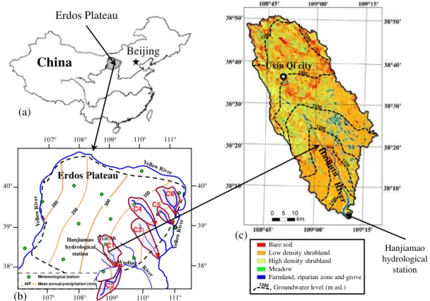
Figure 1.Geographic information of the study site:(a)location of the study area in northern–central China;(b)distribution of meteorological stations in the Erdos Plateau (green points) and the study catchments numbered C1–C6.(c)Characteristics of landscape in catchment C1 (the Hailiutu River catchment) according to Lv et al. (2013).
fied model is calibrated for the study catchments in Sect. 4 and used to produce the annual time series of the evapo-transpiration components linking with the variable soil wa-ter and groundwawa-ter storages. With varying climatic dryness, the shifts of the interannual water balance in the standard and modified Budyko spaces are analyzed and discussed in Sect. 5. The impacts of human activities and the limitations of the approach are also discussed in Sect. 5.
2 Study area, data and preliminary analysis 2.1 River basins
The study area is located in the Erdos Plateau in northern– central China (Fig. 1a), and belongs to the middle part of the Yellow River basin. The climate of the Erdos Plateau is typically inland semiarid to arid with a significant gradient of the mean annual precipitation, from 150 mm in the west to 450 mm in the east (Fig. 1b). More than half of the annual precipitation is received in the warm season (from June to September). Six catchments with available data, numbered C1–C6 (Fig. 1b), are selected for this study. The areas of the catchments range between 1272 and 3253 km2.
In particular, C1 is the Hailiutu River catchment, with an area of 2645 km2, which lies on the southeastern edge of the Mu Us Desert and is a sub-catchment of the Wuding River
basin (Fig. 1b). The main channel in C1 has a length of ap-proximately 85 km and flows southwards to the Hanjiamao hydrological station, as shown in Fig. 1c. Due to the arid cli-mate and desert landscape, the land cover within the catch-ment is characterized by desert sand dunes with patches of mostly shrublands. Depression areas and terraces with shal-low groundwater are covered by meadows and some farm-lands. Wind-breaking trees (Salix matsudanaandPopulus
to-mentosa) can be found along the roads and crop areas.
Farm-lands are mainly located in the southern area and especially in the river valley. Crops cover only∼3 % of the total catch-ment area. Maize is the dominant crop and is irrigated with streamflow and/or groundwater. Several diversion dams have been constructed along the Hailiutu River for irrigation since the early 1970s.
wa-Table 1.The characteristics of the study catchments shown in Fig. 1.
Catchments Area (km2) Mean annual flux*
P(mm) E0(mm) Q(mm) Baseflow index
C1 2645 367 1245 37.7 0.88
C2 2415 386 1218 38.8 0.64
C3 3253 447 1162 127.2 0.72
C4 3065 381 1227 75.8 0.31
C5 1272 466 1146 81.8 0.13
C6 3246 412 1186 53.0 0.16
* According to the data in the 1957–1978 period.
ter conservation projects have been conducted to control the floods and sediment loss. A comparison of the hydrological behaviors between C1 and C6 has been presented by Zhou et al. (2015). In the western part of the Erdos Plateau there are also some river basins, but they lack hydrological data for a proper analysis.
In the study area, groundwater is stored in complex aquifer systems. In general, the Erdos Plateau is character-ized by shallow groundwater in the sandy sediments and deep groundwater in the underlying sandstones. In C1–C2, the Cretaceous sandstones form a thick aquifer enabling ac-tive groundwater circulation. In C3–C6, the Cretaceous sand-stones are limited or replaced by the Jurassic sandstone– mudstone formations with lower permeability so that the movement of deep groundwater is restricted. Meanwhile, shallow groundwater exists in the valleys or near-lake areas covered by sandy or loess sediments. Regional groundwater-level distribution in catchment C1 has been investigated in Lv et al. (2013) based on a hydrogeological survey carried out in 2010 and was shown in Fig. 1c. According to this in-vestigation, the depth to water table (DWT) in C1 varies in a large range from zero to 110 m. In more than half of the area, DWT is less than 10 m. The shallow groundwater zone, where DWT is no more than 2 m, occupies 16.0 % of the whole catchment area. As investigated in Yin et al. (2015) at a research site in this catchment, when DWT is less than 2 m, the actual evapotranspiration is generally 80 % higher than the potential evapotranspiration. This investigation con-firmed that groundwater-dependent evapotranspiration is an essential process in the Erdos Plateau.
2.2 Data
Daily streamflow data since 1957 for the hydrological sta-tions at the outlets of the six catchments were collected from the Yellow River Conservancy Commission (YRCC, 2013). A rainfall gauge was also installed at the Hanjiamao hydro-logical station (Fig. 1c) in 1961, providing daily precipita-tion.
To better account for the variability of rainfall in space and time, we develop gridded monthly precipitation data
with 1 km resolution between 1957 and 2010 from the data of 15 national meteorological stations in the Erdos Plateau (Fig. 1b). Monthly rainfall data at these stations were downloaded from the China Meteorological Adminis-tration (CMA, 2012). We construct the gridded data using the inverse distance square weighting (IDSW) method due to the moderate topography of the Erdos Plateau in the form of low-relief rolling hills. Fig. 1b shows the mean annual precipita-tion contours of the Erdos Plateau obtained from the gridded data. In this study, the area-averaged monthly data of the pre-cipitation in the six catchments for the period 1957–2010 are estimated by imposing the basin boundaries on the gridded monthly precipitation data and taking the arithmetic average of the cell values within the catchment.
The method applied in constructing the gridded precipita-tion data is further applied in constructing a 1 km resoluprecipita-tion gridded data set for the monthly pan evaporation between 1957 and 2010 covering the Erdos Plateau. The pan evapora-tion data were based on observaevapora-tions from 200 mm diameter pans that were installed in most stations in the Erdos Plateau, and can also be downloaded from the CMA dataset (CMA, 2012). The average monthly data of the potential evapotran-spiration (E0)in the six catchments are estimated from the spatially averaged data of the pan evaporation using a local pan coefficient (0.58) for the 200 mm diameter pan. This co-efficient was suggested by various investigations of pan coef-ficients for Chinese meteorological stations (Shi et al., 1986; Fan et al., 2006).
In summary, the mean annual values ofP,E0andQ dur-ing the period in 1957–1978 for the six catchments are listed in Table 1. In this period, the streamflow was not significantly influenced by the hydraulic engineering, irrigation water use and coal mine industry, so that the hydrological behavior was close to the natural state. It can be estimated from the data that the mean annualQ/P values in this “natural” state ranged between 0.1 and 0.3 for the catchments. Accordingly, the mean annualF values are higher than 0.7 with respect to the mean values of the aridity index (E0/P) varying between 2.5 and 3.4.
0 2 4 6 8 10 12
1957 1958 1959 1960 1961 1962 1963 1964 1965 1966 1967 1968 1969 1970 1971 1972 1973 1974 1975 1976 1977 1978 1979 1980 1981 1982 1983 1984 1985 1986 1987 1988 1989 1990 1991 1992 1993 1994 1995 1996 1997 1998 1999 2000 2001 2002 2003 2004 2005 2006 2007 2008 2009 2010
R
unof
f
(m
m
)
Year
Streamflow Baseflow 0
50 100 150 200 250 300
1957 1958 1959 1960 1961 1962 1963 1964 1965 1966 1967 1968 1969 1970 1971 1972 1973 1974 1975 1976 1977 1978 1979 1980 1981 1982 1983 1984 1985 1986 1987 1988 1989 1990 1991 1992 1993 1994 1995 1996 1997 1998 1999 2000 2001 2002 2003 2004 2005 2006 2007 2008 2009 2010
P
o
r
E
0
(
mm)
Year P E0
P
an
d
E0
(mm)
M
o
n
th
ly
ru
n
o
ff
(
m
m
)
(a)
(b)
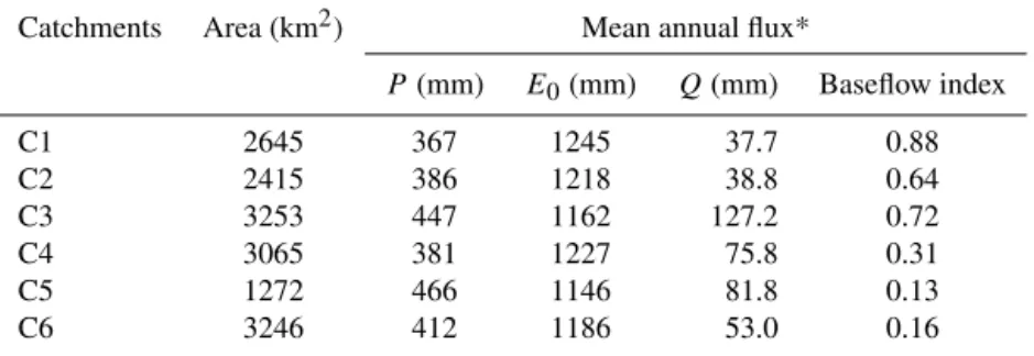
Figure 2.The monthly meteorological data(a)and streamflow–baseflow data(b)from 1957 to 2010 in catchment C1.
Table 2.Mean annual fluxes in the Hailiutu River catchment (C1) in different periods.
Periods P E0 Q Number Of
(mm) (mm) (mm) diversions
(reservoirs)*
1957–1966 387.0 1230.2 42.3 0(0)
1967–1987 337.0 1269.6 32.6 4(2)
1988–1997 329.9 1240.2 23.4 9(2)
1998–2010 352.8 1234.0 28.0 10(2)
* According to Yang et al. (2012).
catchment C1. Both rainfall and evapotranspiration are high in the summer and low in the winter. However, there is a difference in the patterns by which the seasonal variation in runoff may be influenced: the rainfall peak normally ar-rives in August, but the highest evaporation is exhibited in June. With respect to these meteorological patterns, the to-tal runoff drops in the spring and in the early summer until the heavy rainfall comes in August, as shown in Fig. 2b. In comparison with the rainfall and the potential evapotranspi-ration, the mean monthly runoff (2.6 mm) and its fluctuation amplitude (0.8–11.9 mm) are quite small. This indicates that most of the precipitation in C1 returns to the atmosphere by evapotranspiration. During 1957–2010, the annual aridity in-dex in the catchment showed a large variation range (between 1 and 10), covering the semi-humid, semi-arid and arid cli-matic conditions as classified in the scheme recommended by the United Nations Environment Programme (UNEP) (Mid-dleton and Thomas, 1992).
In the study area, there are significant interannual fluctua-tions in streamflow. For catchment C1, Yang et al. (2012) in-vestigated the annual regime shifts in streamflow and found that the shifts were caused largely by land use policy changes and river water diversions for irrigation. Table 2 shows the mean annual fluxes in four typical periods with different
numbers of water diversions in the Hailiutu River and ma-jor branches during 1957–2010. These diversions influenced the hydrological behavior in C1 and will be discussed in the following sections. However, before 1967, the Hailiutu River was free of hydraulic engineering, and the studied area was mostly close to the natural conditions. In the other catchments, the changes in the streamflow regime were also mainly contributed by human activities but in more com-plex ways. In C6, the river discharge was also influenced by a large number of check dams that were constructed to re-duce water and sediment loss (Zhou et al., 2015). In C3–C5, the impacts of the coal mining industry were significant. To analyze the natural hydrological behaviors, the study period should not be later than 1978.
2.3 Preliminary analysis using (P−Q)/P
In many cases, it is possible to estimate the annualEin a catchment from the annually observedP andQbyP−Q
when the change in storage is significantly small. Then it could be treated as the “real” data of the annualEand the shift of annual water balance in the Budyko space could be investigated with the plot of (P−Q)/Pvs.ϕ. In this section, we check the validity of this approach in the study area.
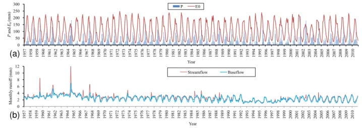
The plots of annual (P−Q)/P vs.ϕ during 1957–1878 (close to the natural state) for the six catchments are shown in Fig. 3. In particular, Fig. 3a shows the locations of the mean annual (P−Q)/Pdata of the six catchments in the Budyko space. The data points fall below the original Budyko curve given by Eq. (2), but can be bounded between two modified Budyko curves that are determined using Eq. (3). They ap-proximately exhibit a positive relation between (P−Q)/P
andϕ. This indicates that the behaviors of the catchments on a long-term average (22 years) satisfied the steady-state wa-ter balance assumption in the original Budyko framework.
0.0 0.2 0.4 0.6 0.8 1.0 1.2
0 2 4 6 8 10
(
P
-Q
)/
P
Aridity index
0 2 4 6 8 10
0.0 0.2 0.4 0.6 0.8 1.0 1.2
Aridity index
(
P
-Q
)/
P
C1 −0.03
0 2 4 6 8 10 0.0
0.2 0.4 0.6 0.8 1.0 1.2
Aridity index
(
P
-Q
)/
P
C2
C3
0 2 4 6 8 10 0.0
0.2 0.4 0.6 0.8 1.0 1.2
Aridity index
(
P
-Q
)/
P
0 2 4 6 8 10 0.0
0.2 0.4 0.6 0.8 1.0 1.2
Aridity index
(
P
-Q
)/
P
0 2 4 6 8 10 0.0
0.2 0.4 0.6 0.8 1.0 1.2
Aridity index
(
P
-Q
)/
P
(c)
(d) (e) (f )
0.00 0.02
−0.01
−0.06 −0.02 (a)
C5
C4 C6
(b)
w=1.6
w= 2.5
C1–C6
Figure 3.The plots of the annual (P−Q)/P data vs. the aridity index in the study catchments for the 1957–1978 period:(a)the mean annual data points for the six catchments bounded by the two Budyko curves (dashed lines) according to Eq. (3) withw=1.6 andw=2.5; and(b–f)are the annual data points of the different catchments. C1–C6 are the numbers of the catchments shown in Fig. 1. The solid line is the original Budyko curve determined with Eq. (2). The dashed lines are the regression curves of the scatter data points with the slope values shown nearby.
in each catchment should be an increasing curve with a positive slope in the Budyko space. However, as shown in Fig. 3b–d, the annual (P−Q)/P data in C1–C4 follow a negative relation. The annual (P−Q)/Pvalue of C3 signif-icantly decreased from∼0.8 to∼0.5 when the aridity index increased from 1.2 to 5.8 (Fig. 3c). It seems that C5 (Fig. 3e) and C6 (Fig. 3f) showed a positive relation, but the data points did not fall closely along the original Budyko curve. The negative relations in C1–C4 are contrary to the posi-tive relation in the original Budyko framework, indicating the falseness of taking the annual (P−Q)/P as the replica of the annualF value in the study area. In a previous study, Istanbulluoglu et al. (2012) also highlighted this abnormal relation in the North Loup River basin, Nebraska, USA, and they demonstrated that it was caused by ignoring the change in storage. They used long-term monitoring data of ground-water level to estimate the interannual change in groundwa-ter storage (1G) and replaced the (P−Q)/P data with the
(P−Q−1G)/P data to reproduce a normal Budyko curve
for the basin. However, groundwater-dependent evapotran-spiration was not explicitly considered in Istanbulluoglu et al. (2012).
It is a good idea to estimate the change in groundwater storage using groundwater monitoring data. However, long-term groundwater-level monitoring data are not available for the catchments in this study. In addition, the approach of us-ing (P−Q−1G)/P data ignores the interannual change in
the soil moisture storage. In a different way from Istanbullu-oglu et al. (2012), we estimate1Gfrom the monthly base-flow (groundwater discharge) data with a calibrated hydro-logical model, into which the groundwater-dependent evapo-transpiration is also incorporated. Using the model, the stor-age components and the contribution of groundwater for the annualE can be simultaneously obtained at the catchment scale.
3 Hydroclimatologic models 3.1 The ABCD model
The ABCD model is a conceptual hydrological model with four parameters (a,b,c, andd) developed by Thomas (1981) to account for the actual evapotranspiration, surface/sub-surface runoff and storage changes. The ABCD model was originally applied at an annual time step but has been rec-ommended as a monthly hydrological model (Alley, 1984). It was widely applied as a hydroclimatologic model to in-vestigate the response of catchments to climate change (Van-dewiele et al., 1992; Fernandez et al., 2000; Sankarasubrama-nian and Vogel, 2002; Li and SankarasubramaSankarasubrama-nian, 2012).
W
G
P E
cR
Q (1−c)R
dG
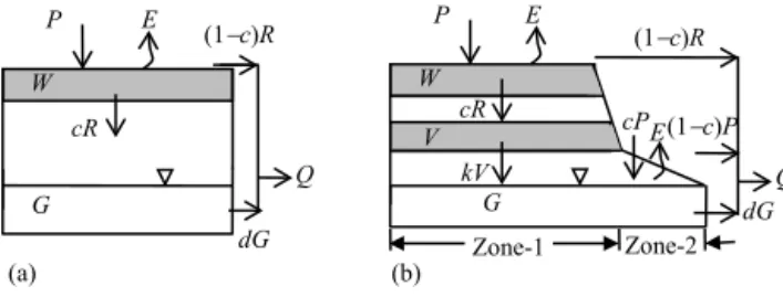
(a) (b)
Zone-1 W
P E
G
cPE
Q
Zone-2 (1−c)P
dG cR
V kV
(1−c)R
Figure 4.Schematic representations of the ABCD model(a)and ABCD-GE model(b).WandVare the effective soil water storage and the effective storage in the transition vadose zone, respectively. Gis the effective groundwater storage.
Wm−Wm-1=Pm−Em−Rm, (4)
whereWm-1andWm are the effective soil water storages at the beginning and at the end of themth month, respectively;
PmandEmare the monthly precipitation and evapotranspi-ration, respectively; andRmis the monthly loss of soil water via direct runoff and groundwater recharge. The change in groundwater storage is determined by
Gm−Gm-1=cRm−dGm, (5)
whereGm-1andGmrepresent the groundwater storage at the beginning and end of the mth month, respectively;candd
are two parameters that account for groundwater recharge and discharge from Rm andGm, respectively. The monthly streamflow is the summation of the monthly direct runoff and groundwater discharge, as follows:
Qm=(1−c)Rm+dGm. (6)
The change in storage in the ABCD model is the summation of the changes in the soil water storage and groundwater stor-age, which can be expressed as (Wm−Wm-1)+(Gm−Gm-1). Thomas (1981) proposed a nonlinear function to estimate (Em+Wm)from (Pm+Wm-1)as follows:
Em+Wm=
Pm+Wm-1+b
2a −
s
P
m+Wm-1+b 2a
2
−(Pm+Wm-1)b
a , (7)
whereais a dimensionless parameter andbis the upper limit of (Em+Wm). In addition, Thomas (1981) assumed that
Wm=(Em+Wm)exp(−E0m/b), (8)
whereE0mis the monthly potential evaporation for themth month. Substituting Eq. (8) into Eq. (7), the monthly
evapo-transpiration can be estimated as
Em=
P
m+Wm-1+b 2a −
s
Pm+Wm-1+b
2a
2
−(Pm+Wm-1)b a
1−exp
−E0m
b
. (9)
Wang and Tang (2014) demonstrated that Eq. (9) can be de-rived from the generalized proportionality principle and yield an equivalent Budyko-type model.
3.2 The ABCD-GE model
To investigate the effect of groundwater-dependent evapo-transpiration in basins with both shallow and deep ground-water, the original ABCD model is extended in this study as the ABCD-GE model, where “GE” denotes groundwater-dependent evapotranspiration. As shown in Fig. 4b, a catch-ment is conceptually divided into two zones where Zone-1 and Zone-2 represent different areas with deep and shallow groundwater, respectively. Direct runoff originates from both zones. Surface water (water in river, canals, lakes, etc.) is also included in Zone-2. The soil water reservoir in Zone-1 is the same as that in the ABCD model. In addition, a transition va-dose zone is specified between the soil layer and water table to represent the delayed groundwater recharge. The transition zone is included to handle the existence of the thick unsatu-rated zone (> 10 m) in a basin. Soil water in this zone is dom-inated by the vertical downward flow. In Zone-2, the rafall and evapotranspiration are the components directly in-volved in the water balance of groundwater. Thus, three stor-age components are considered as a chain in the hydrological processes. It is assumed that the potential change in ground-water storage by the lateral flow coming in and out of a catch-ment is negligible. For a large river basin (> 1000 km2)this assumption is generally acceptable.
ABCD-GE model, this zone could not be influenced by both the evapotranspiration and groundwater flow processes. Thus, the thickness of the soil layer would be less than 2 m in the model. However, one should be aware that it is not necessary to find the distinct and exact boundaries for the zones, since the ABCD-GE model is a conceptual hydrological model.
Similar to that in the ABCD model, the change in the soil water storage in Zone-1 is determined by
Wm−Wm-1=Pm−E1m−Rm, (10)
whereE1mis the monthly evapotranspiration in Zone-1 de-termined with Eq. (9); Rm becomes the summation of the leaking soil water to the transition vadose zone,cRm, and the direct runoff, (1−c)Rm, in Zone-1. The change in storage of the vadose zone is described with
Vm−Vm-1=cRm−kVm, (11)
whereVmandVm-1represent the values of the storage in the transition vadose zone at the end and beginning of themth month, respectively, andkis the parameter that accounts for the groundwater recharge rate askVm.
In the ABCD-GE model, the source of runoff is partitioned by the fractions of the area of the two zones. The total runoff in the catchment is the summation of the direct runoff and groundwater discharge as follows:
Qm=(1−α)(1−c)Rm+α(1−c)Pm+dGm, (12)
whereαis the ratio of the Zone-2 area to the whole catch-ment area. In Eq. (12), the term (1−α)(1−c)Rm denotes the direct runoff contributed by Zone-1, whereas the term
α(1−c)Pm denotes the direct runoff contributed by Zone-2. In considering the gain–loss processes of groundwater, the change in the effective groundwater storage is yielded by
Gm−Gm-1=(1−α)kVm+α(cPm−E2m)−dGm, (13)
where E2m is the monthly evapotranspiration in Zone-2, which depends on the effective groundwater storage as fol-lows:
E2m=gGmE0m, (14)
where g is a parameter controlling the intensity of groundwater-dependent evapotranspiration. Eq. (14) as-sumes that the evapotranspiration rate in Zone-2 is simply proportional to both the groundwater storage (which is posi-tively related to groundwater level) and the potential evap-otranspiration rate. Thus, the evapevap-otranspiration rate as a whole in the catchment is summarized as
Em=(1−α)E1m+αE2m. (15)
Eqs. (10)–(13) are solved one by one and finally the value of Gmis substituted into Eq. (12) to obtain the runoff. The results of the ABCD-GE model are controlled by seven pa-rameters as a,b,c,d,g,kandα. The parameter values can be identified with the model calibration process.
4 Model calibration and results 4.1 Model calibration
We apply the ABCD-GE model to estimate the monthly evapotranspiration and the change in the storage compo-nents in the six catchments after the model parameters were calibrated. The monthly evapotranspiration data are then summed up to estimate the annual evapotranspiration for fur-ther analysis. The model calibration is based on the observed monthly streamflow data at the hydrological stations and the separated baseflow data.
Because groundwater discharge has been included in the model, a baseflow analysis was performed to obtain the ex-pected groundwater discharge for the model calibration. Us-ing the HYSEP automated hydrograph separation method (Sloto and Crouse, 1996) on the daily streamflow data, such “observed” groundwater discharge data were obtained. For C1, these data were partly reported in Zhou et al. (2013). The mean values of the baseflow index for C1–C6 range be-tween 0.13 and 0.88 (Table 1). Catchment C1 has the highest baseflow index (0.88), indicating that groundwater discharge is the dominant hydrological process in this catchment. Vari-ation patterns of the monthly groundwater discharge in C1 are shown in Fig. 2b. In C5 and C6, the baseflow index val-ues are smaller than 0.2 because most of the streamflow in the two catchments is contributed by direct runoff.
The ordinary least squares (OLS) criterion is applied for parameter estimation. The errors of both log-streamflow and log-baseflow were included in the OLS objective function, as follows:
minU= N X
m=1
e2m+qm2
, (16)
where
em=ln(Q/Q)ˆ m, qm=ln(Qˆb/Qb)m (17)
For catchment C1, the model parameters are firstly identi-fied using the 1957–1966 data, and this calibrated model is considered to be a “natural” model due to the minimum im-pact of human activities during this 10-year period. For C2– C6, the 1957–1978 period is applied to roughly identify the “natural” model. The initial storage values are treated as the unknown parameters to be determined in the calibration pro-cess. Changes in the initial conditions generally influenced the simulated results in the first and second years. Therefore, the residual errors in the later years are applied to estimate the parameter values with less influence from the initial con-ditions. A sensitivity analysis is carried out to schematically capture the ranges of the parameter values.
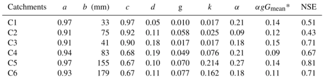
The best fitting parameter values of the “natural” models for C1–C6 are shown in Table 3. The a value ranges be-tween 0.91 and 0.97. In previous studies using the ABCD model, theavalue was generally found to be higher than 0.9 (Alley, 1984; Sankarasubramanian and Vogel, 2002; Li and Sankarasubramanian, 2012). Thebandcvalues in this study are generally higher than those obtained by Alley (1984) for 10 catchments in the USA. The highercvalue indicates the more significant role of groundwater in the hydrological be-haviors. However, thedvalues of C1–C6 fall into the range suggested by Alley (1984). The optimized α values in the “natural” models range between 0.09 and 0.27. In particu-lar, theαvalue of C1 (0.21) in this “natural” state was larger than the current value (DWT in 16.0 % of the area is less than 2 m). Such a difference is reasonable because the groundwa-ter level in the 1950s and 1960s should be higher than that at present, as indicated by the higher baseflow (Fig. 2b). The
kvalue controls the rate of groundwater recharge below the transition vadose zone. The transition vadose zone is a neces-sary component in C1–C3, as demonstrated by the sensitivity analysis. When an extremely high value ofkis used (k> 100), the kVm value would be almost equal to cRm, so that the transition vadose zone does not make sense. However, in this situation the model could not capture the seasonal vari-ation patterns of groundwater discharge. Thus, the delayed groundwater recharge is an essential process for the catch-ments. The best fittingkvalues for C4–C6 are significantly higher than those for C1–C3, indicating a weaker delay ef-fect. This confirms the hydrogeological conditions in C4–C6: active groundwater flow is limited in the near-surface zone.
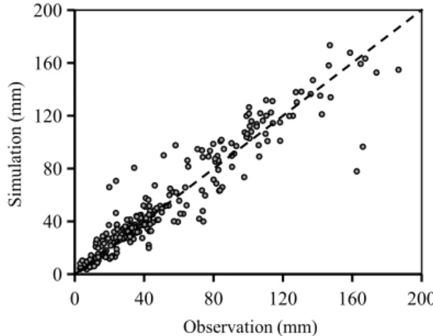
For the calibration period, the root-mean-square error (RMSE) of the “natural” models with respect to the aggre-gated results of the six catchments is 39 % for the monthly runoff. For the aggregated annual runoff data, the RMSE is 21 %. The errors include the streamflow observation er-ror and the meteorological data treatment erer-ror. It is more reasonable to evaluate the model performance according to the observation–simulation correlation coefficient and the NSE value. A comparison between the observed and simu-lated monthly runoff (including groundwater discharge) for all of the six catchments can be seen in Fig. 5. The coef-ficient of determination (R2=0.89) is high. The NSE
val-0 40 80 120 160 200
0 40 80 120 160 200
Observation
S
imu
la
tio
n
Observation (mm)
S
imu
la
ti
o
n
(
mm)
Figure 5.Scatter plot for the observation and simulation results of the monthly runoff and groundwater discharge in the study catch-ments in the calibration period.
ues of the model range between 0.48 and 0.81 for the differ-ent catchmdiffer-ents (Table 3), indicating that the model performs well in the study area. It is usually difficult to obtain a high NSE value for a catchment with weak seasonal variation in runoff (Mathevet et al., 2006), such as that in C1 and C2. 4.2 Modeling results
We use the “natural” models to estimate the monthly hydro-logical components during the whole 1957–2010 period. As an example, typical results of catchment C1 are shown in Fig. 6. The modeling results of the monthly runoff after the 1970s are generally higher than the observed data (Fig. 6a) due to one ignoring the impacts of land use changes and in-creased utilization of water for irrigation. However, the sim-ulated patterns of groundwater discharge are similar to the observations (Fig. 6b): falling in the summer, rising in the winter. This agreement between the simulated and observed patterns demonstrates the ability of the ABCD-GE model in simulating the hydrological behaviors in the studied catch-ment: significant groundwater-dependent evapotranspiration occurs in the summer, and a strong recovery of storage in the shallow-groundwater zone occurs in the winter due to de-layed recharge from the thick vadose zone.
For catchment C1, there are significant differences be-tween the observed and model-calculated annual runoff after 1966, as shown in Fig. 6c. This deviation could be interpreted as the excess evapotranspiration induced by the increasing agricultural water use. Enhanced evapotranspiration also oc-curred in the shallow groundwater zone due to groundwater pumping for irrigation. To evaluate the actual water balance, the following equation,
EACT≈ENAT+(QNAT−QOBS), (18)
Table 3.Best fitting parameters of the “natural” models for the study catchments.
Catchments a b (mm) c d g k α αgGmean* NSE
C1 0.97 33 0.97 0.05 0.010 0.017 0.21 0.14 0.51
C2 0.91 75 0.92 0.11 0.058 0.025 0.09 0.12 0.43
C3 0.91 41 0.90 0.18 0.017 0.017 0.18 0.15 0.71
C4 0.94 83 0.68 0.19 0.049 0.076 0.21 0.09 0.67
C5 0.97 155 0.67 0.10 0.070 0.214 0.27 0.14 0.81
C6 0.93 179 0.67 0.11 0.077 0.162 0.18 0.11 0.71
*Gmeanis the mean value of the effective groundwater storage in the calibration period.
0 2 4 6 8 10
1957 1958 1959 1960 1961 1962 1963 1964 1965 1966 1967 1968 1969 1970 1971 1972 1973 1974 1975 1976 1977 1978 1979 1980 1981 1982 1983 1984 1985 1986 1987 1988 1989 1990 1991 1992 1993 1994 1995 1996 1997 1998 1999 2000 2001 2002 2003 2004 2005 2006 2007 2008 2009 2010
Qb
(mm)
Year
Observation Simulation
0 2 4 6 8 10
1957 1958 1959 1960 1961 1962 1963 1964 1965 1966 1967 1968 1969 1970 1971 1972 1973 1974 1975 1976 1977 1978 1979 1980 1981 1982 1983 1984 1985 1986 1987 1988 1989 1990 1991 1992 1993 1994 1995 1996 1997 1998 1999 2000 2001 2002 2003 2004 2005 2006 2007 2008 2009 2010
Q
(mm)
Year
Observation Simulation
0 10 20 30 40 50 60 70
1957 1962 1967 1972 1977 1982 1987 1992 1997 2002 2007
Runoff (mm)
Year
Observation Simulation
(a)
(b)
(c)
200 250 300 350 400
1957 1962 1967 1972 1977 1982 1987 1992 1997 2002 2007
E
(mm)
Year Actrual ET "Natural" model
(d)
1957 1962 1967 1972 1977 1982 1987 1992 1997 2002 2007
1957 1962 1967 1972 1977 1982 1987 1992 1997 2002 2007
Year
Year
Actual ET ""
Figure 6.Simulated results of the “natural” ABCD-GE model in comparison with the observation data in catchment C1 from 1957 to 2010, including monthly runoff(a), groundwater discharge(b), annual runoff(c)and annual evapotranspiration(d). The actual evapotranspiration in(d)was estimated with Eq. (18).
result (ENAT) plus the difference of the annual runoff be-tween the “natural” model (QNAT) and the observation (QOBS). This difference may be partly induced by the multi-ple timescale variations in the climate conditions, but would be mainly caused by the irrigation water use. Results are shown in Fig. 6d. It seems that the relative difference be-tween ENAT and EACT is not significant. The maximum
de-0 2 4 6 8 10 0.0
0.5 1.0 1.5 2.0 2.5
Aridity index
E
/
P
0 2 4 6 8 10 0.0
0.5 1.0 1.5 2.0 2.5
Aridity index
E
/
P
0 2 4 6 8 10 0.0
0.5 1.0 1.5 2.0 2.5
Aridity index
E
/
P
0 2 4 6 8 10 0.0
0.5 1.0 1.5 2.0 2.5
Aridity index
E
/
P
0 2 4 6 8 10 0.0
0.5 1.0 1.5 2.0 2.5
Aridity index
E
/
P
0 2 4 6 8 10 0.0
0.5 1.0 1.5 2.0 2.5
Aridity index
E
/
P
C1 C2 C3
C4 C5 C6
0.17
0.14 0.16
0.08 0.10 0.08
F F F
F F F
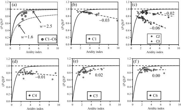
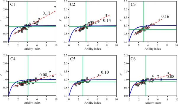
Figure 7. Plots of the annualF−ϕ data in the study catchments in the standard Budyko space for the 1957–2010 period. The actual evapotranspiration is estimated using the “natural” models. The solid blue line is the original Budyko curve determined with Eq. (2). The dashed red lines are the linear regression curves of the data points with the slope data shown nearby. The intersection point of the green lines denotes the mean annual data.
creased even though the seasonal patterns basically remained (Fig. 6b).
4.3 Annual water balance in the standard Budyko space
In Fig. 7, the annualF data for the annual water balance ob-tained from the “natural” models over the 1957–2010 period are plotted in the standard Budyko space. It is obvious that with the increasing aridity index (ϕ), the evapotranspiration ratio (F) for all of the catchments increased in almost a lin-ear pattern with the different slopes. Whenϕ< 4, most of the data points fall below the original Budyko curve, indicating thatF< 1 is generally satisfied in this situation. Whenϕ> 4, the original Budyko curve givesF ≈1, indicating the limi-tation (0 <F ≤1) for the mean annual evapotranspiration ra-tio. However, some of the data points fall above the line of
F =1, whileϕis larger than 3 but even less than 4, indicat-ing that theF> 1 cases did not only occur in dry years. The maximumF value (2.2) was obtained in C1 when the arid-ity index jumped fromϕ=1.5 in 1964 toϕ=9.8 in 1965. This means that C1 lost a volume of water in 1965 by evap-otranspiration that is more than twice the gained water from precipitation in the same year. In comparison, the F values in C4 and C6 are not sensitive to the change in the aridity index since the slopes of theF−ϕ regression lines are less than 0.1.
The effect of groundwater-dependent evapotranspiration can be clearly observed when the evapotranspiration ratio
is divided into two parts and plotted in the Budyko space separately with respect to the shallow and deep groundwater zones. The annualEvalues in Zone-1 and Zone-2 are esti-mated, respectively, as
E1=
12
X
m=1
E1m(Wm-1, a, b) and E2=
12
X
m=1
E2m(Gm, g) (19)
for every year, whereE1mis calculated with Eq. (9), whereas
0 2 4 6 8 0
1 2 3 4
E0 /P
E
/
P
E1/P E2/P
0 2 4 6 8
0 1 2 3 4
E0 /P
E
/
P
E1/P E2/P
F=φ
Eq. (3),w=1.4 F= 0.52φ+0.24
F=φ
F= 0.13φ+0.64
Eq. (3),w= 1.6
C1 C4
Budyko, 1958
F
Aridity index Aridity index
F
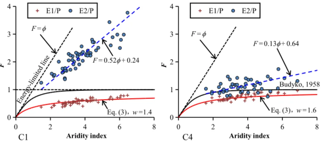
Figure 8.Plots of theF−ϕdata in the standard Budyko space using theE1data for Zone-1 and theE2data for Zone-2 that estimated with
Eq. (19) in catchments C1 (left) and C4 (right). The red curves are the Budyko curves determined with Eq. (3), which could approximately represent the variations of theE1/P data. The dashed blue lines are the linear regression lines of theE2/P data.
In catchment C1, the E2/P data points follow a lin-ear regression line with a slope of 0.52. This agrees with the relationship between E2 andE0 (E2∝E0) that is de-scribed in Eq. (14). Since the groundwater storage,G, is rel-atively stable (small d andkvalues in the model), the an-nualE2/P value would be proportional to theϕ value and the slope is close to the annual mean value of gG. In C1, the annual mean value ofgGis 0.65 according to the “natu-ral” model. Such a groundwater-dependent evapotranspira-tion process is the reason for the occurrence of the F > 1 cases at the catchment scale. Note that in the original Budyko framework, theF =ϕcase denotes an energy-limited condi-tion when water supply (only precipitacondi-tion for mean annual water balance) is sufficient for the evapotranspiration pro-cess. The slope of theE2/P line in C1 is less than 1.0, but is closer to theF =ϕline than the water-limited line repre-sented byF =1. It indicates that in Zone-2 the evapotranspi-ration process is in a quasi-energy-limited condition, rather than in a water-limited condition, because shallow ground-water can effectively serve as an external source of ground-water supply.
In C4, the E2/P data points show a scatter distribution around the regression line. This is mainly caused by the significant variability in the groundwater storage, G, at the monthly and annual scales. Thedandkvalues in the model for C4 are quite larger than that for C1 by which the model could capture the significant fluctuation of the baseflow. As a result, the annual meangGvalues of C4 vary in a large range between 0.18 and 0.84. Similar unstableE2/P data also ex-ist for C5 and C6 as indicated by the high d andkvalues (Table 3).
5 Discussions
5.1 Controls on theF> 1 cases
It has been demonstrated in Fig. 7 that the annual evapotran-spiration ratio,F, could be higher than 1.0 when the aridity index,ϕ, is larger than 4.0 in the studied catchments. In the literature, theF> 1 cases were also observed whenϕis just higher than 1.0 (Cheng et al., 2011; Wang, 2012; Chen et al., 2013). Thus, it is interesting to discuss how the occurrence of theF> 1 cases is controlled by the catchment properties when shallow groundwater plays an important role.
The equation for the annual evapotranspiration ratio can be derived from Eqs. (15) and 19) as follows:
F =(1−α)E1
P +αg
E0
P
12
X
m=1
E0m
E0
Gm
, (20)
where the term E0m/E0 denotes the proportion of the monthly potential evaporation to the annual one with respect to themth month. It has been known that the relationship between E1/P and ϕ determined by the ABCD model is similar to that predicted by the standard Budyko formulas, as shown in Fig. 8, where E1/P is less than 1.0. For the groundwater-dependent term, defining
Ga=
12
X
m=1
E
0m
E0
Gm
(21)
as the weighted average of the monthly groundwater storage, Eq. (20) can be replaced by
F (ϕ)=(1−α)[1+ϕ−(1+ϕw)1/w] +αgGaϕ, (22)
whereE1/P is represented by Eq. (3). According to Eq. (22), the functionF(ϕ)is controlled by the parameters, g,w,α
and the status of groundwater represented byGa. As
de-0 2 4 6 8 10 0
1 2
F
Cachments data
0 2 4 6 8 10
0 1 2
F
Cachments data
α= 0.1
α= 0.1
(a) (b)
α= 0.5
α= 0.9
α= 0.5
α= 0.9
α= 0.1
α= 0.5
α= 0.1 α= 0.9
α= 0.5
α= 0.9
Catchments data Catchments data
Aridity index Aridity index
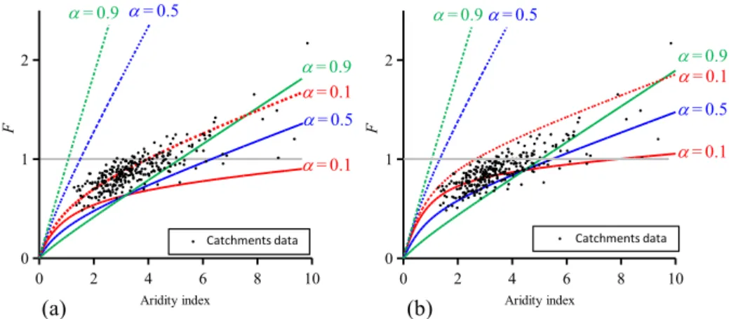
Figure 9.The typicalF−ϕcurves for annual water balance in the standard Budyko space determined with Eq. (22) whenw=1.5(a) and w=2.0(b). The solid and dashed curves are estimated usinggGa=0.2 andgGa=1.0, respectively. Dots are the data points of the study catchments.
scribe the intensity of groundwater-dependent evapotranspi-ration related to the potential evapoevapotranspi-ration. The recommended range of gGa is 0.2–1.0 according to Table 3. In Eq. (22),
the term with w indicates the normal energy-water-limited process in Zone-1, whereas the term withgGaindicates the
quasi-energy-limited process in Zone-2. The actualF value is a mixed result of the different processes.
Typical F−ϕ curves obtained with Eq. (22) are plot-ted in Fig. 9. It can be seen that the proportion of shal-low water table area (α) has a large effect on the occur-rence of theF> 1 case. When the shallow water table area is small (α=0.1), theF> 1 case occurs only during dry years. When thegGa value increases, theF> 1 case occurs at the
smaller aridity index. The specific catchment parameter (w) for E1/P also influences the occurrence of the F> 1 case. A largerwvalue shifts theF−ϕcurves (comparing Fig. 9b with a) to the left side, indicating that the F> 1 case could occur at the smaller aridity index.
Groundwater-dependent evapotranspiration estimated in the ABCD-GE model does not violate theF< 1 rule for the long-term steady-state water balance, because the model will yieldE=P−Qfor the average flux in a long-term period. As shown in Fig. 9, more than half of the data points fall below the line ofF =1, indicating that the less-than-1 rule for the averageF value is satisfied in the whole study area. For each catchment, in addition, the mean annualF−ϕdata for the 1957–2010 period have been shown in Fig. 7 (inter-section points of the green cross lines). None of these mean annualF values is higher than 1.
5.2 Using effective precipitation and the modified Budyko space
The standard Budyko space assumes that the potential water supply for evapotranspiration is only rainfall in a catchment. This is valid for the mean annual water balance, but excep-tions might exist for the annual or intra-annual behaviors.
Several previous studies attempted to modify the Budyko framework for the short timescale. Wang (2012) and Chen et al. (2013) argued that the reduction of storage in a pe-riod should be regarded as one of the water supply com-ponents. They suggested an approach to replace the evapo-transpiration ratio and the aridity index byE/(P−1S) and
E0/(P−1S), respectively, where1S is the storage deple-tion in a studied period andP−1S is regarded as the ef-fective precipitation. In this modified Budyko space, evapo-transpiration is always less than the water supply, so that the original Budyko hypothesis could be satisfied for the small timescale problems. Alternatively, Greve et al. (2016) pro-posed a two-parameter Budyko function to explain the cases of evapotranspiration exceeding precipitation in unsteady-state conditions. However, groundwater flow is not included in their model, so that the role of groundwater-dependent evapotranspiration could not be assessed by such a two-parameter Budyko function.
In this section, we attempt to check the characteristics of the annual water balance data in the study area using the modified Budyko space suggested by Wang (2012) and Chen et al. (2013). With the results of the ABCD-GE model, the total change in storage for a year can be estimated as
1S=
12
X
m=1
[(1−α)(Wm+Vm−Wm-1−Vm-1)
+(Gm−Gm-1)], (23)
wheremis the number of the months in the year,W0,V0and
G0form=0 denoting the respective storage components at the end of the previous year.
0 2 4 6 0.0
0.2 0.4 0.6 0.8 1.0
E0/(P-dS)
0 2 4 6 0.0
0.2 0.4 0.6 0.8 1.0
E0/(P-dS)
0 2 4 6 0.0
0.2 0.4 0.6 0.8 1.0
E0/(P-dS)
E
/(
P-d
S
)
0 2 4 6 0.0
0.2 0.4 0.6 0.8 1.0
E0/(P-dS)
0 2 4 6 0.0
0.2 0.4 0.6 0.8 1.0
E0/(P-dS)
0 2 4 6 0.0
0.2 0.4 0.6 0.8 1.0
E0/(P-dS)
C1 C2 C3
C4 C5 C6
w= 2.5
w=1.9
E
/(
P-d
S
)
E
/(
P-d
S
)
E
/(
P-d
S
)
E
/(
P-d
S
)
E
/(
P-d
S
)
Figure 10.The annual water balance data in the modified Budyko space with the effective precipitation defined by Wang (2012). Dots are the data obtained for the catchments using the “natural” models. The solid curves represent the standard Budyko curves determined with Eq. (3) usingE0/(P−1S) andE/(P−1S), respectively, instead ofF andϕ. Budyko curves ofw=1.9 andw=2.5 are selected to bound
the data points of catchment C1 and applied for the comparison with the other catchments. The dashed lines approximately represent the limitations of theE/(P−1S) data.
the cases in C1 and C2, the increase in E/(P−1S) with the increasingE0/(P−1S) seems too small in comparison with any one of the standard Budyko curves determined by Eq. (3). A similar difference between the data and the stan-dard Budyko curves also exists in the other catchments, but is not as significant as that in C1 and C2. Furthermore, in C1 and C2 theE/(P−1S) value approaches a stable value around 0.90 with the highE0/(P−1S) values. It indicates that at least 10 % of P−1S is contributed to the annual runoff in terms of Q/(P−1S). This portion of the water supply seems to be inaccessible for the evapotranspiration process. Similar bounds of theE/(P−1S) value also exist in C3–C6. In particular, this limitation is lower than 0.8 in C3, implying a significant contribution of change in storage to the streamflow in dry years.
The difficulties in using the effective precipitation defined by Wang (2012) and Chen et al. (2013) are the unknown1S
for an investigated time step and the possible existence of the inaccessible part of 1S for the evapotranspiration pro-cess. Consequently, the estimation of theE/(P−1S) value is not straightforward, but requires a complex iteration pro-cess. In the original Budyko framework for the steady-state water balance, the water supply (only precipitation) does not depend on both evapotranspiration and runoff, so that the aridity index is an independent variable in assessing the behaviors of the catchments. However, the water sup-ply represented by the effective precipitation is influenced by
the evapotranspiration–runoff processes due to the feedback mechanism. This interdependence between the water supply and evapotranspiration significantly reduces the efficiency of using the modified Budyko space in analyzing the shift of an-nual water balance in a catchment. In contrast, it would be an efficient and straightforward approach to extend formulas for annual water balance in the standard Budyko space, such as Eq. (22), keeping an independent index (ϕ)for the climatic conditions.
5.3 Landscape-driven and human-controlled shifts of annual water balance
Along the river, the area of the surface water body was sig-nificantly enlarged in the reservoirs, leading to an increase in the surface water evapotranspiration loss. It is equivalent to the increase in groundwater-dependent evapotranspiration in this study because surface water is also included in the shallow groundwater zone. As a result, the shift of the an-nual water balance in the Budyko space was partly caused by change in land use and controlled by regulation of river water for irrigation.
Recently, Jaramillo and Destouni (2014) developed a method to assess the landscape-driven change in the mean evapotranspiration ratio using the difference between the ac-tual change in theF value and the climate-driven change in the F value following the Budyko framework. In this sec-tion, we extend their method to assess the landscape-driven change in annual water balance in catchment C1. The period between 1957 and 1966 is selected from Table 2 as the ref-erence period. Changes are evaluated for the different aver-age values of the annualF data in the different periods listed in Table 2. The climate-driven change is estimated with the annualENATvalues obtained from the “natural” model, us-ing a formula similar to Jaramillo and Destouni (2014), as follows:
1
E
LD
P
=1
E
ACT
P
−1
E
NAT
P
, (24)
where 1(ELD/P) denotes the landscape-driven change in comparison with the 1957–1966 period. However, this quan-tity index includes the landscape changes driven by both the climatic force and human activities. To check how this index is correlated with the increasing impacts from the reservoirs and diversions in rivers, following Jaramillo and Destouni (2015), the coefficient of intra-annual vari-ation of the monthly runoff (CVQ) was applied. The CVQ/CVP value was estimated to reveal the separate
influ-ence of such a human-controlled flow regulation from the mixed human-climate controlling, whereCVP is the
coeffi-cient of intra-annual variation of the monthly rainfall. Results of the1(ELD/P) and1(CVQ/CVP)data between
the three periods 1968–1987, 1988–1997, and 1998–2010 and the reference period 1957–1967 are shown for catch-ment C1 in Fig. 11. The 1(ELD/P) values are all pos-itive but not big (less than 6 %), indicating a slight in-crease in the evapotranspiration ratio after 1966 driven by the changes in the natural landscape conditions of water storage and/or human-controlled land use. The 1(CVQ/,CVP)
val-ues show a significant fluctuation around zero, but are also limited in a small range (±5 %). Both the 1(ELD/P) and
1(CVQ/CVP) values are largest in 1988–1997.
Fluctua-tions of these data could not be fully explained by the in-creasing number of diversions in the rivers. The negative
1(CVQ/CVP) value in 1968–1987 may be caused by the
construction of two reservoirs since reservoirs commonly smooth the variation of the streamflow. In 1988–1997, the
1(CVQ/CVP)value became positive when five new
diver--2 -1 0 1 2 3 4 5 6
A
bno
rm
a
li
ty
(%)
系列1
系列2
1967–1987 1988–1997 1998–2010
Δ(ELD/P)
Δ(CVQ /CVP)
4(2)
9(2)
10(2)
Figure 11. Histogram of the 1(ELD/P) data determined with
Eq. (24) and the1(CVQ/CVP)data determined with the coeffi-cients of intra-annual variation of the monthly runoff (CVQ)and rainfall (CVP)for the different periods in catchment C1. The num-bers of diversions (reservoirs) are shown on the top of the blocks according to Table 2.
sions were built, indicating the opposite impacts of the reser-voirs and diversions. It is possible that the streamflow was disturbed by the regulation of water for irrigation on these diversions with small overflow dams. The decrease in the
1(CVQ/CVP)value from 4.72 % in 1988–1977 to 0.72 % in
1998–2010 may be caused by the control of the river water use under some government policies to prevent desertifica-tion (Yang et al., 2012; Zhou et al., 2015). The following de-crease in the1(ELD/P) value from 5.05 % in 1988–1997 to 3.73 % in 1998–2010 is not significant, seemingly indicating the alternative irrigation practice in the croplands (for exam-ple, pumping groundwater), so that the real water consump-tion was reduced but still on a high level. As a result, uti-lization of surface water and groundwater for irrigation can increase the frequency of theF> 1 cases.
5.4 Limitation remarks
Attention should be paid to the simplifications in the con-ceptual model extended from the ABCD model, when the equations and formulas are applied in complicated catchments. The ABCD model assumes that the storage– evapotranspiration relationship is controlled by the param-etersaandb, whereas the physical interpretation of them is difficult (Alley, 1984). Eq. (8) in the ABCD model is also hypothesized from a simplified storage-loss model that is controlled by the parameterb(Thomas, 1981). Sankarasub-ramanian and Vogel (2002) suggested that theb value for the annual water balance could be approximately represented by the maximum soil moisture field capacity plus the maxi-mumE0forϕ< 1 or the maximumP forϕ≥1. Theavalue is generally estimated in a small range between 0.95 and 1.0. In this study, the model output is not sensitive to the
groundwater-dependent evapotranspiration that has been incorporated into the ABCD-GE model. The ABCD-GE model divides the area into shallow and deep groundwater zones, without con-sidering a complicated spatial distribution of groundwater depth. For the shallow groundwater zone, the evapotranspi-ration is assumed to be proportional to the groundwater stor-age. Nonlinear behavior in groundwater-dependent evapo-transpiration could be further included if it can be success-fully parameterized. A linear groundwater storage–discharge relationship is adopted in both of the ABCD and ABCD-GE models. These simplifications could cause systematic errors in modeling a catchment where the nonlinear behaviors in the hydrological processes are significant.
Limitations in the data processing and complexities in the hydrogeological conditions could also influence the accuracy of the modeling results. The average potential evapotranspi-ration data,E0, and the average precipitation data,P, in some degree, are dependent on the estimation methods and may in-troduce biases. For the hydrogeological conditions, this study assumed that the boundary of a catchment determined along the terrain divides is also the boundary of groundwater flow; i.e., no inter-basin transfer of groundwater exists. The as-sumption is plausibly acceptable in the eastern part of the Erdos Plateau because the spatial variation in the groundwa-ter level is highly correlated with the land surface elevation in this area (Lv et al. 2013; Zhou et al., 2015). However, the groundwater flow system in the western part of the Erdos Plateau is more complex, where the climate is more arid and water table divides could be significantly different from the terrain divides.
In fact, when the Budyko framework is applied for small timescale water balance in a catchment, the other addi-tional sources of water supply should be considered, apart from groundwater. Significant changes in soil moisture, snow cover or frozen water in cold regions could also cause an “ab-normal” shift of the annual water balance for a catchment in the standard Budyko space (Jaramillo and Destouni, 2014). The effects of these storage components are negligible in this study, but may be essential in other study areas. In particular, the special processes in the cold regions are not included in the ABCD-GE model. However, one can refer to Martinez and Gupta (2010), where the snow-augmented ABCD model was proposed and can be incorporated into an extension of the ABCD-GE model.
6 Conclusions
The Budyko framework was developed for the long-term steady-state water balance in catchments, which estimates the evapotranspiration ratio (F) as a function of the aridity index (ϕ). It can be represented by curves for theF−ϕ rela-tionship in the standard Budyko space that were determined by the original Budyko formula without any parameter or the formulas with a catchment-specific parameter. It is interest-ing to investigate whether the Budyko space can also be
ap-plied to capture the annual water balance in a catchment with varying dryness. However, the shift of the annual water bal-ance in the standard Budyko space could be significantly dif-ferent from that presumed from the standard Budyko curves, in particular, when the cases ofF> 1 occur as have been ob-served in a number of catchments.
In this study, we highlight the effect of groundwater-dependent evapotranspiration in triggering the abnormal shift of the annual water balance in the standard Budyko space. A conceptual monthly hydrological model, the ABCD-GE model, is developed from the widely used ABCD model to incorporate groundwater-dependent evapotranspiration into the zone with a shallow water table and delayed groundwater recharge into the zone with a deep water table. The model is successfully applied to analyze the behaviors of six catch-ments in the Erdos Plateau, China.
The results show that the standard Budyko formulas are not applicable for the interannual variability of catchment water balance when groundwater-dependent evapotranspira-tion is significant. The shift of the annual water balance in the
F−ϕ space is a combination of the Budyko-type response in the deep groundwater zone and the quasi-energy-limited condition in the shallow groundwater zone. Shallow ground-water supplies excess evapotranspiration during dry years, leading to theF > 1 cases. The occurrence of theF > 1 cases depends on the proportion area of the shallow groundwater zone, the intensity of groundwater-dependent evapotranspi-ration and the catchment properties determining the Budyko-typeF−ϕ relationship in the deep groundwater zone. Wa-ter utilization for irrigation may enhance this excess evapo-transpiration phenomenon. The modified Budyko space with the effective precipitation incorporating the change in stor-age can forceF values below 1.0. However, the computa-tion is complicated in dealing with the gain–loss feedback and uncertain with the inaccessible storage for the evapo-transpiration process. The empirical formula proposed in this study for the standard Budyko space provides a straightfor-ward method for predicting the changes in the annual water balance with the varying dryness.
7 Data availability
Acknowledgements. This study is supported by the Program for New Century Excellent Talents in University (NCET) that was granted by the Ministry of Education, China, and partly supported by the Honor Power Foundation, UNESCO-IHE. The authors are grateful to the constructive comments from R. Donohue, F. Jaramillo and the other anonymous reviewers.
Edited by: R. Moussa
Reviewed by: R. Donohue, F. Jaramillo, and three anonymous referees
References
Alley, W. M.: On the treatment of evapotranspiration, soil moisture accounting, and aquifer recharge in monthly water balance mod-els, Water Resour. Res., 20, 1137–1149, 1984.
Arora, V. K.: The use of the aridity index to assess climate change effect on annual runoff, J. Hydrol„ 265, 164–177, 2002. Budyko, M. I.: Evaporation under natural conditions, Isr. Program
for Sci. Transl., Jerusalem, Isreal, 1948.
Budyko, M. I.: The heat balance of the earth’s surface, US Depart-ment of Commerce, Washington, D.C., USA, 1958.
Budyko, M. I.: Climate and life, Academic, New York, USA, 1974. Chen, X. and Hu, Q.: Groundwater influences on soil moisture and
surface evaporation, J. Hydrol., 297, 285–300, 2004.
Chen, X., Alimohammadi, N., and Wang, D.: Modeling interannual variability of seasonal evaporation and storage change based on the extended Budyko framework, Water Resour. Res., 49, 6067– 6078, doi:10.1002/wrcr.20493, 2013.
Cheng, L., Xu, Z., Wang, D., and Cai, X.: Assessing interannual variability of evapotranspiration at the catchment scale using satellite-based evapotranspiration data sets, Water Resour. Res., 47, W09509, doi:10.1029/2011WR010636, 2011.
CMA (China Meteorological Administration): Monthly land sur-face climatic dataset in China, Climatic Data Center, Na-tional Meteorological Information Center, CMA, Beijing, China, available at: http://data.cma.cn/data/index/6d1b5efbdcbf9a58. html (last access: 9 July 2016) 2012.
Cohen, D., Person, M., Daannen, R.,Sharon, L., Dahlstrom, D., Za-bielski, V., Winter, T. C., Rosenberry, D. O., Wright, H., Ito, E., Nieber, J., and Gutowski Jr., W. J.: Groundwater-supported evap-otranspiration within glaciated watersheds under conditions of climate change, J. Hydrol., 320, 484–500, 2006.
Donohue, R. J., Roderick, M. L., and McVicar, T. R.: On the impor-tance of including vegetation dynamics in Budyko’s hydrological model, Hydrol. Earth Syst. Sci., 11, 983–995, doi:10.5194/hess-11-983-2007, 2007.
Fan, J., Wang, Q., and Hao, M.: Estimation of reference crop evap-otranspiration by Chinese pan, Transactions of the CSAE, 22, 14–17, 2006. (in Chinese)
Fernandez, W., Vogel, R. M., and Sankarasubramanian, A.: Re-gional calibration of a watershed model, Hydrol. Sci. J., 45, 689– 707, 2000.
Fu, B. P.: On the calculation of the evaporation from land surface, Sci. Atmos. Sin., 5, 23–31, 1981. (in Chinese)
Gentine, P., D’Odorico, P., Lintner, B. R., Sivandran, G., and Salvucci, G.: Interdependence of climate, soil, and vegetation
as constrained by the Budyko curve, Geophys. Res. Lett., 39, L19404, doi:10.1029/2012GL053492, 2012.
Gerrits, A. M. J., Savenije, H. H. G., Veling, E. J. M., and Pfister, L.: Analytical derivation of the Budyko curve based on rainfall characteristics and a simple evaporation model, Water Resour. Res., 45, W04403, doi:10.1029/2008wr007308, 2009.
Greve, P., Gudmundsson, L., Orlowsky, B., and Seneviratne, S. I.: Introducing a probabilistic Budyko framework, Geophys. Res. Lett., 42, 2261–2269, 2015.
Greve, P., Gudmundsson, L., Orlowsky, B., and Seneviratne, S. I.: A two-parameter Budyko function to represent conditions under which evapotranspiration exceeds precipitation, Hydrol. Earth Syst. Sci., 20, 2195–2205, doi:10.5194/hess-20-2195-2016, 2016.
Istanbulluoglu, E., Wang, T., Wright, O. M., and Lenters, J. D.: In-terpretation of hydrologic trends from a water balance perspec-tive: The role of groundwater storage in the Budyko hypothesis, Water Resour. Res., 48, W00H16, doi:10.1029/2010WR010100, 2012.
Jaramillo, F. and Destouni, G.: Developing water change spec-tra and distinguishing change drivers worldwide. Geophys. Res. Lett., 41, 8377–8386, 2014.
Jaramillo, F. and Destouni, G.: Local flow regulation and irrigation raise global human water consumption and footprint, Science, 350, 1248–1251, 2015.
Koster, R. D. and Suarez, M. J.: A Simple framework for examin-ing the interannual variability of land surface moisture fluxes, J. Climate, 12, 1911–1917, 1999.
Li, W. and Sankarasubramanian, A.: Reducing hydrologic model uncertainty in monthly streamflow predictions using mul-timodel combination, Water Resour. Res., 48, W12516, doi:10.1029/2011WR011380, 2012.
Lv, J., Wang, X.-S., Zhou, Y., Qian, K., Wan, L., Derek, E., and Tao, Z.: Groundwater-dependent distribution of vegetation in Hailiutu River catchment, a semi-arid region in China, Ecohydrology, 6, 142–149, 2013.
Martinez, G. F. and Gupta, H. V.: Toward improved iden-tification of hydrological models: A diagnostic evaluation of the “abcd” monthly water balance model for the con-terminous United States, Water Resour. Res., 46, W08507, doi:10.1029/2009WR008294, 2010.
Mathevet, T., Michel, C., Andreassian, V., and Perrin, C.: A bounded version of the Nash-Sutcliffe criterion for better model assessment on large sets of basins, In: Large Sample Basin Ex-periments for Hydrological Model Parameterization: Results of the Model Parameter Experiment–MOPEX, IAHS Publ., 307, 211–218, 2006.
Mezentsev, V. S.: More on the calculation of average total evapora-tion, Meteorol. Gidrol., 5, 24–26, 1955.
Middleton, N. and Thomas, D. S. G.: World atlas of desertification, United Nations Environment Programme, Edward Arnold, 1992. Nash, J. E. and Sutcliffe, J. V.: River flow forecasting through con-ceptual models part I – A discussion of principles, J. Hydrol., 10, 282–290, 1970.
Porporato, A., Daly, E. and Rodriguez-Iturbe, I.: Soil water balance and ecosystem response to climate change, Am. Nat., 164, 625– 632, 2004.