www.hydrol-earth-syst-sci.net/20/771/2016/ doi:10.5194/hess-20-771-2016
© Author(s) 2016. CC Attribution 3.0 License.
The cost of ending groundwater overdraft on the North China Plain
Claus Davidsen1,2,3, Suxia Liu2, Xingguo Mo2, Dan Rosbjerg1, and Peter Bauer-Gottwein1
1Technical University of Denmark, Department of Environmental Engineering, Kgs. Lyngby, Denmark
2Chinese Academy of Sciences, Key Laboratory of Water Cycle and Related Land Surface Processes, Institute of Geographic
Sciences and Natural Resources Research, Beijing, China
3Sino-Danish Center for Education and Research, Aarhus, Denmark
Correspondence to:Claus Davidsen ([email protected]), Suxia Liu ([email protected]), and Peter Bauer-Gottwein ([email protected])
Received: 28 April 2015 – Published in Hydrol. Earth Syst. Sci. Discuss.: 22 June 2015 Revised: 14 December 2015 – Accepted: 26 January 2016 – Published: 19 February 2016
Abstract.Overexploitation of groundwater reserves is a ma-jor environmental problem around the world. In many river basins, groundwater and surface water are used conjunctively and joint optimization strategies are required. A hydroeco-nomic modeling approach is used to find cost-optimal sus-tainable surface water and groundwater allocation strategies for a river basin, given an arbitrary initial groundwater level in the aquifer. A simplified management problem with con-junctive use of scarce surface water and groundwater un-der inflow and recharge uncertainty is presented. Because of head-dependent groundwater pumping costs the optimization problem is nonlinear and non-convex, and a genetic algo-rithm is used to solve the one-step-ahead subproblems with the objective of minimizing the sum of immediate and ex-pected future costs. A real-world application in the water-scarce Ziya River basin in northern China is used to demon-strate the model capabilities. Persistent overdraft from the groundwater aquifers on the North China Plain has caused declining groundwater levels. The model maps the marginal cost of water in different scenarios, and the minimum cost of ending groundwater overdraft in the basin is estimated to be CNY 5.58 billion yr−1. The study shows that it is
cost-effective to slowly recover the groundwater aquifer to a level close to the surface, while gradually lowering the ground-water value to the equilibrium at CNY 2.15 m−3. The model
can be used to guide decision-makers to economic efficient long-term sustainable management of groundwater and sur-face water resources.
1 Introduction
Groundwater aquifers are of high economic importance around the world and often act as buffers in the water sup-ply system during droughts (Tsur and Graham-Tomasi, 1991; Tsur, 1990). On the North China Plain, persistent ground-water overexploitation over the past decades has caused de-cline of the shallow and deep groundwater tables (Liu et al., 2001). The immediate benefits of satisfying the water de-mands greatly exceed the costs of pumping, which highlights the problem of the present self-regulating management. As the groundwater resource is overexploited, the immediate benefits of the increased unsustainable supply have to be traded off against the long-term increase in pumping costs and reduced buffering capacity. Optimal allocation of the wa-ter resources should address coordinated use of the wawa-ter re-sources by considering the long-term total costs, while utiliz-ing the groundwater as a buffer. This is in line with the 2011 Chinese No. 1 Policy Document, which targets improvement of water use efficiency and reduction of water scarcity (CPC Central Committee and State Council, 2010).
represen-tation of the groundwater system using spatially distributed groundwater models (Andreu et al., 1996; Harou and Lund, 2008; Marques et al., 2006; Pulido-Velázquez et al., 2006). Stochasticity is commonly represented in scenarios where a regression analysis is used to formulate operation rules; see e.g., the implicit stochastic optimization approaches re-viewed by Labadie (2004). Singh (2014) rere-viewed the use of simulation–optimization (SO) modeling for conjunctive groundwater and surface water use. In SO-based studies, ef-ficient groundwater simulation models are used to answer “what if” questions, while an optimization model is wrapped around the simulation model to find “what is best”. Ground-water aquifers have been represented as simple deterministic box or “bathtub” models (e.g., Cai et al., 2001; Riegels et al., 2013) and as spatially distributed models (e.g., Maddock, 1972; Siegfried et al., 2009) with stochasticity (Reichard, 1995; Siegfried and Kinzelbach, 2006). While the results ob-tained from these methods are rich in detail, they yield only a single solution to the optimization problem.
Methods based on dynamic programming (DP, Bellman, 1957) have been used extensively to demonstrate the dynam-ics of conjunctive groundwater–surface water use for both deterministic (e.g., Buras, 1963; Provencher and Burt, 1994; Yang et al., 2008) and stochastic DP (SDP, e.g., Burt, 1964; Philbrick and Kitanidis, 1998; Provencher and Burt, 1994; Tsur and Graham-Tomasi, 1991) optimization problems. In DP-based methods, the original optimization problem is de-composed into subproblems, which are solved sequentially over time. The entire decision space is thereby mapped, en-abling use of the results as dynamic decision rules. How-ever, the number of subproblems grows exponentially with the number of state variables and this curse of dimensional-ity has frequently limited the use of DP and SDP (Labadie, 2004; Provencher and Burt, 1994; Saad and Turgeon, 1988). Although it causes loss of detail and inability to disaggre-gate the results, reservoir aggregation has been suggested as a possible solution strategy (Saad and Turgeon, 1988).
This study aims to answer the following two macroscale decision support questions for conjunctive groundwater and surface water management for the Ziya River basin in North China. (1) What are the minimum costs of ending ground-water overdraft? (2) What is the cost-efficient recovery strat-egy of the overpumped aquifer? A hydroeconomic model-ing approach is used to identify the least-cost strategy to achieve sustainable groundwater abstraction, defined as the term average abstraction that does not exceed the long-term average recharge. To overcome the management prob-lem similar to Harou and Lund (2008) with increased com-plexity caused by uncertain surface water runoff and ground-water recharge, the surface ground-water reservoirs are aggregated. This is adequate at a macroscale (Davidsen et al., 2015) and allows the use of DP-based approaches. The cost minimiza-tion problem is solved with the water value method, a vari-ant of SDP (Stage and Larsson, 1961; Stedinger et al., 1984) which produces dynamic tables of marginal costs linked to
states, stages, and water source. Head- and rate-dependent pumping costs introduce nonlinearity in the discrete subprob-lems. This nonlinearity is handled with a hybrid genetic al-gorithm (GA) and linear programming (LP) method similar to that used by Cai et al. (2001), here applied in a coupled groundwater–surface water management problem within an SDP framework.
2 Methods 2.1 Study area
Northern China and particularly the North China Plain (NCP) have experienced increasing water scarcity problems over the past 50 years due to population growth, economic de-velopment, and reduced precipitation (Liu and Xia, 2004). The deficit in the water balance has historically been covered by overexploitation of the groundwater aquifer, causing a re-gional lowering of the groundwater table by up to 1 m yr−1
(Zheng et al., 2010).
The Ziya River basin, a part of the Hai River basin, was se-lected as a case study area (see Fig. 1). The upper basin is lo-cated in the Shanxi province, while the lower basin is lolo-cated in the Hebei province on the NCP. The 52 300 km2basin has approximately 25 million inhabitants (data from 2007, Bright et al., 2008), and severe water scarcity is causing multiple conflicts. Five major reservoirs with a combined storage ca-pacity of 3.5 km3 are located in the basin. While reservoir rule curves and flood control volumes can easily be accom-modated for in the optimization approach, current reservoir management rule curves in the case area are unavailable to the public. Instead it is assumed that the full storage capac-ity can be managed flexibly without consideration of storage reserved for flood protection or existing management rules. Incorporating flood storage volumes will reduce the available storage and increase water scarcity in the long dry season. In the present model setup, we therefore find the lower limit on water scarcity costs, assuming that the entire storage capac-ity is available for storing water. Reservoir spills will cause an economic loss, and the model tends to avoid spills by en-tering the rainy season with a low reservoir storage level.
A previous hydroeconomic study of the Ziya River basin was a traditional implementation of SDP on a single-reservoir system (surface water single-reservoir) and showed opti-mal water management, while disregarding dynamic ground-water storage and head-dependent groundground-water pumping costs (Davidsen et al., 2015). Instead, the groundwater re-source was included as a simple monthly upper allocation constraint.
±
Baiyangdian Lake Yellow River SHANXI PROVINCE HEBEI PROVINCE SHANDONG PROVINCE Bohai Gulf Legend Basin boundary Rivers/canals Major city SNWTP Province border Lakes/reservoirs Calibration basin 117°E 116°E 115°E 114°E 113°E 38°N 37°N 39°N Shijiazhuang Xinzhou Tianjin Beijing ! ! ! ! ! ! !0 50 100 km
Figure 1.The Ziya River basin. Watershed and rivers automatically delineated from a digital elevation map (USGS, 2004) and manu-ally verified and corrected with Google Earth (Google Inc., 2013). The SNWTP routes (central and eastern) were sketched in Google Earth and verified with field observations. Provincial boundaries from NGCC (2009).
the SDP framework. We therefore set up a box model for the downstream and most important aquifer only, and ab-straction from the upstream aquifer is only bounded by an upper pumping limit corresponding to the average monthly recharge. The box model for the downstream aquifer is formulated as Infiltration+Storage=Pumping+Overflow. The groundwater overflow is only used in extreme cases, where the total pumping and available storage is less than the infiltration. The spills will go to the spill variable and leave the system as baseflow to the rivers (unavailable for allocation). The aquifer is so heavily overexploited that no significant baseflow is being created or will be created in the foreseeable future. The box model allows for more flexi-ble management with large abstractions in dry years and in-creased recharge in wet years. The groundwater aquifer can thereby be used to bridge longer drought periods. Except for the groundwater box model, the conceptual model is identi-cal to the one used by Davidsen et al. (2015).
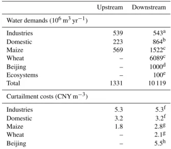
A conceptual sketch of the management problem is shown in Fig. 2. The water users are divided into groups of eco-nomic activities; irrigation agriculture, industrial users, and domestic water users. Ideally, each water user group should be characterized by flexible demand curves, but due to poor data availability a constant water demand (m3)and a con-stant curtailment cost of not meeting the demand were used for each group (see Table 1). The water demands are assumed to be deterministic and decoupled from the stochastic runoff. This is a reasonable assumption because the rainfall on the NCP normally occurs in the summer months, while irrigation water demands are concentrated in the dry spring. The irri-gation schedule is centrally planned and typically unchanged from year to year. The upstream (u) users have access to runoff and are restricted to an upper pumping limitXgw
cor-Table 1.Annual water demands and curtailment costs for the users in the Ziya River basin. Based on the data set from Davidsen et al. (2015).
Upstream Downstream
Water demands (106m3yr−1)
Industries 539 543a Domestic 223 864b
Maize 569 1522c
Wheat – 6089c
Beijing – 1000d
Ecosystems – 100e Total 1331 10 119
Curtailment costs (CNY m−3)
Industries 5.3 5.3f Domestic 3.2 3.2f
Maize 1.8 2.8g
Wheat – 2.1g
Beijing – 5.5h
aDemands scaled by area, (Berkoff, 2003; Moiwo et al., 2010;
World Bank, 2001).
bBased on daily water demand (National Bureau of Statistics of China, 2011)
scaled by the 2007 population from Landscan (Bright et al., 2008).
cBased on the land cover (USGS, 2013) and irrigation practices collected in the
field. The wheat irrigation demand is evenly distributed in March, April, May, and June. Maize is irrigated in July.
dBased on the plan by The People’s Government of Hebei Province (2012),
Ivanova (2011).
eEstimated deficit in the Baiyangdian Lake (Mo, 2006). fEstimated by World Bank (2001).
gBased on the water use efficiency (Deng et al., 2006) and producers’ prices
(USDA Foreign Agricultural Service, 2012). hEstimated by Berkoff (2003).
u1 u2
Xgw xsw,u 1 xgw,u 1 xsw,u 2 xgw,u 2 ssw rsw qsn Qw Vmax,gw Vgw Vmax,sw
Qsw qE
d1 d4
d2 d3 xsw,d
1
xgw,d 1
∆hThiem
∆htop
∆h
xgw,d 2 xgw,d3 xsw,d 2 xsw,d 3 Qgw xsn d x4
Figure 2.Conceptual sketch of the simplified water management problem. Water users are located upstream (u) and downstream (d) of a surface water reservoir. Allocation decision variables for sur-face water (blue), SNWTP water (green), and groundwater (orange) are indicated. The conceptual sketch of the downstream dynamic aquifer shows how the total lift (1h) is composed of the thickness of the top layer, the regional groundwater drawdown, and the local Thiem steady-state groundwater drawdown.
2.2 Optimization model formulation
An SDP formulation is used to find the expected value of storing an incremental amount of surface water or ground-water, given the month of the year, the available storage in surface and groundwater reservoirs, and the inflow scenar-ios. The backward recursive equation calculates the sum of immediate and expected future costs for all combinations of discrete reservoir storage levels (states) and monthly time steps (stages). The immediate management cost (IC) arises from water supply and water curtailment, whereas the ex-pected future cost (EFC) is the optimal value function int+1 weighed by the corresponding transition probabilities. In the present setup, we decided to weigh the IC and EFC equally, but inclusion of discount rates other than zero is possible. Be-cause of the head- and rate-dependent groundwater pumping costs, which will be described in detail later, the immediate cost depends nonlinearly on the decision variables. The ob-jective is to minimize the total costs over the planning period, given by the optimal value functionF∗
t Vgw, t, Vsw, t, Qksw, t
based on the classical Bellman formulation: Ft∗
Vgw,t, Vsw,t, Qksw,t
=
min IC
Vgw,t, Vsw,t, Qksw,t
+ L X
l=1
pklFt∗+1
Vgw,t+1, Vsw,t+1, Qlsw,t+1
, (1)
with IC being
IC
Vgw, t, Vsw, t, Qksw, t
= M X
m=1
cswxsw+cgwxgw
+cSNWTPxSNWTP+cctxct)m, t
−rsw, tbhp, (2)
subject to
xsw, m, t+xgw, m, t+xSNWTP, m, t+xct, m, t=dmm, t (3)
Vsw, t+Qsw, t− U X
u=1
xsw, u, t−rsw, t−sgw, t=Vgw,t+1 (4)
rsw, t+ssw, t= D X
d=1
xsw, d, t+qE, t (5)
Vgw, t+Qgw, t− D X
d=1
xgw, d, t−sgw, t=Vgw, t+1 (6)
U X
u=1
xsw, u, t≤Qsw, t (7)
U X
u=1
xgw, u, t≤Xgw, t (8)
rt≤R, xsw,Bei+xSNWTP,Bei≤QSNWTP,
qE, t≥QE, Vsw, t≤Vmax, sw, Vgw, t≤Vmax, gw (9)
cgw=f Vgw, D X
d=1
xsw, d !
. (10)
See Table 2 for nomenclature.
Equation (3) is the water demand fulfillment constraint; i.e., the sum of water allocation and water curtailments equals the water demand of each user. Equation (4) is the water balance of the combined surface water reservoir, while Eq. (5) is the water balance of the reservoir releases. A sim-ilar water balance for the dynamic groundwater aquifer fol-lows in Eq. (6). The upstream surface water allocations are constrained by the upstream runoff as shown in Eq. (7), while the upstream groundwater allocations are constrained to a fixed sustainable monthly average as shown in Eq. (8). In Eq. (9), the upper and lower hard constraints on the decision variables are shown. Lastly, Eq. (10) is the marginal ground-water pumping cost, which depends on the combined down-stream groundwater allocations as described later.
A rainfall–runoff model based on the Budyko Framework (Budyko, 1958; Zhang et al., 2008) has been used in a pre-vious study to estimate the near-natural daily surface wa-ter runoff into reservoirs (Davidsen et al., 2015). The re-sulting 51 years (1958–2008) of simulated daily runoff was aggregated to monthly runoff and normalized. A Markov chain, which describes the runoff serial correlation between three flow classes defined as dry (0–20th percentile), nor-mal (20–80th percentile), and wet (80–100th percentile), was established and validated to ensure second-order stationar-ity (Davidsen et al., 2015; Loucks and van Beek, 2005). The groundwater recharge is estimated from the precipita-tion data also used in the rainfall–runoff model. The average monthly precipitation (mm month−1) for each runoff class is
calculated, and a simple groundwater recharge coefficient of 17.5 % of the precipitation (Wang et al., 2008) is used.
The SDP loop is initiated with EFC set to zero and will propagate backward in time through all the discrete system states as described in the objective function. For each discrete combination of states, a cost minimization subproblem will be solved. A subproblem will have the discrete reservoir stor-age levels (Vgw, t andVsw, t)as initial conditions and
Table 2.Nomenclature.
F∗
t optimal value function in staget(2005 Chinese Yuan, CNY)
Vgw, t stored volume in the groundwater aquifer, decision variable (m3)
Vsw, t stored volume in the surface water reservoir, decision variable (m3)
Vmax,sw upper storage capacity, surface water reservoir (m3)
Vmax,gw upper storage capacity, groundwater aquifer (m3)
Qsw, t river runoff upstream reservoirs, stochastic variable (m3month−1)
Qgw, t groundwater recharge, assumed to be perfectly correlated withQsw, t(m3month−1)
m indicates theMwater users
gw groundwater
sw surface water
ct water curtailments
x allocated volume, decision variable (m3month−1)
c marginal costs (CNY m−3); the costs are all constants, except for
cgw which is correlated to the specific pump energy; see Eq. (11)–(16)
rt reservoir releases through hydropower turbines, decision variable (m3month−1)
R upper surface water reservoir turbine capacity (m3month−1)
ssw reservoir releases exceedingR, decision variable (m3month−1)
bhp marginal hydropower benefits (CNY m−3)
k indexes theKinflow classes in staget l indexes theLinflow classes int+1
pkl transition probability fromktol dmm water demand for userm(m3month−1)
u indexes theUupstream users
d indexes theDdownstream users
sgw spills from aquifer whenVgw, t+Qsw, t−xgw, t> Vmax,sw(m3month−1)
Xgw maximum monthly groundwater pumping in the upstream basin (m3month−1)
qE, t unused surface water available to ecosystems, decision variable (m3month−1)
QE minimum in-stream ecosystem flow constraint (m3month−1)
Bei Beijing user
QSNWTP maximum capacity of the SNWTP canal (m3month−1)
the Markov chain transition probabilities. The algorithm will continue backward in time until equilibrium is reached, i.e., until the shadow prices (marginal value of storing water for future use) in two successive years remain constant. The SDP model is developed in MATLAB (MathWorks Inc., 2013) and uses the fast cplexlp (IBM, 2013) to solve the linear sub-problems.
The sets of equilibrium shadow prices, referred to as the water value tables, can subsequently be used to guide optimal water resources management forward in time with unknown future runoff. In this study, the available historic runoff time series is used to demonstrate how the derived water value ta-bles should be used in real-time operation. The simulation will be initiated from different initial groundwater aquifer storage levels, thereby demonstrating which pricing policy should be used to bring the NCP back into a sustainable state. 2.3 Dynamic groundwater aquifer
The groundwater aquifer is represented as a simple box model (see Fig. 2) with recharge and groundwater pumping determining the change in the stored volume of the aquifer
(Eq. 6). The pumping is associated with a pumping cost de-termined by the energy needed to lift the water from the groundwater table to the land surface (Eq. 10):
P =(ρg1h) /ε, (11)
whereP is the specific pump energy (J m−3),ρ is the
den-sity of water (kg m−3), g is the gravitational acceleration
(m s−2),1his the head difference between groundwater
ta-ble and land surface (m), andεis the pump efficiency (−). The marginal pumping costcgw (CNY m−3)is found from
the average electricity pricecel(CNY/Ws) in northern China:
cgw=celP . (12)
Hence this cost will vary with the stored volume in the groundwater aquifer. The present electricity price structure in China is quite complex, with the users typically paying between CNY 0.4 and 1 kWh−1depending on power source,
province, and consumer type (Li, 2012; Yu, 2011). In this study a fixed electricity price of CNY 1 kWh−1is used. The
immediate costs of supplying groundwater to a single user follow
where1his found as the mean depth from the land surface to the groundwater table (see Fig. 2) betweentandt+1:
1h=1htop+
Vmax,gw−
Vgw, t+Vgw, t+1
2
S−1
y A−1, (14)
where1htopis the distance from the land surface to the top
of the aquifer at full storage (m), Sy is the specific yield
(−) of the aquifer, and A is the area of the aquifer (m2). HereVgw, t+1is a decision variable, and once substituted into
Eq. (13) it is clear that the problem becomes nonlinear. In Eq. (14) the drawdown is assumed uniform over the en-tire aquifer. This simplification might be problematic as the local cone of depression around each well could contribute significantly to the pumping cost and thereby the optimal policy. Therefore, the steady-state Thiem drawdown (Thiem, 1906) solution is used to estimate local drawdown at the pumping wells. Local drawdown is then added to Eq. (15) to estimate total required lift:
1hThiem=
Qw
2π T ln
rin
rw
, (15)
whereQw is the pumping rate of each well (m3month−1),
T is the transmissivity (m2month−1), r
in is the radius of
influence (m), and rw is the distance from origin to the
point of interest (m), which here is the radius of the well. The transmissivity is based on a hydraulic conductivity of 1.3×10⁻⁶m s−1 for silty loam (Qin et al., 2013). The
hy-draulic conductivity is lower than the expected average for the NCP to provide a conservative estimate of the effect of drawdown. Field interviews revealed that the wells typi-cally reach no deeper than 200 m below surface, which re-sults in a specific yield of 5 %. The groundwater pumping Qw is defined as the total allocated groundwater within the
stage (m3month−1) and assumed evenly distributed among
the number of wells in the catchment:
Qw, t= D P
d=1
xgw, d, t
nw
=Vgw, t−Vgw, t+1+Qgw, t−sgw, t
nw
, (16) wherenw is the number of wells in the downstream basin.
The even pumping distribution is a fair assumption, as field investigations showed that (1) the majority of the groundwa-ter wells are for irrigation; (2) the timing of irrigation, crop types, and climate is homogeneous; and (3) the groundwa-ter wells have comparable capacities. Erlendsson (2014) es-timated the well density in the Ziya River basin from Google Earth to be 16 wells km−2. Assuming that the wells are
dis-tributed evenly on a regular grid and that the radius of in-fluence rin is 500 m, overlapping cones of depression from
eight surrounding wells are included in the calculation of the local drawdown. This additional drawdown is included us-ing the principle of superposition as also applied by Erlends-son (2014).
2.4 Solving nonlinear and non-convex subproblems With two reservoir state variables and a climate state vari-able, the number of discrete states is quickly limited by the curse of dimensionality. A very fine discretization of the groundwater aquifer to allow discrete storage levels and deci-sions is computationally infeasible. A low number of discrete states increases the discretization error, particularly if both the initial and the end storagesVgw, t+1andVsw, t+1are kept
discrete. The discrete volumes of the large aquifer become much larger than the combined monthly demands, and stor-ing all recharge will therefore not be sufficient to recharge to a higher discrete storage level. Similarly, the demands will be smaller than the discrete volumes, and pumping the remain-ing water to reach a lower discrete level would also be infea-sible. Allowing free end storage in each subproblem will al-low the model to pick, e.g., the optimal groundwater recharge and pumping without a requirement of meeting an exact dis-crete end state. With free surface water and groundwater end storages, the future cost function has three dimensions (sur-face water storage, groundwater storage, and expected future costs). Pereira and Pinto (1991) used Benders’ decomposi-tion approach, which employs piecewise linear approxima-tions and requires convexity. With head- and rate-dependent pumping costs and increasing electricity price, we observed that the future cost function changes from strictly convex (very low electricity price) to strictly concave (very high electricity price). At realistic electricity prices, we observed a mix of concave and convex shapes. An alternative is to use linear interpolation with defined upper and lower bounds. However, with two state variables, interpolation between the future cost points will yield a hyperplane in three dimensions, which complicates the establishment of boundary conditions for each plane.
Nonlinear optimization problems can be solved with evo-lutionary search methods, a subdivision of global optimiz-ers. A widely used group of evolutionary search methods are genetic algorithms (GAs), which are found to be efficient tools for getting approximate solutions to complex nonlinear optimization problems (see, e.g., Goldberg, 1989; Reeves, 1997). GAs use a random search approach inspired by nat-ural evolution and have been applied to the field of water resources management by, e.g., Cai et al. (2001), McKinney and Lin (1994), and Nicklow et al. (2010). Cai et al. (2001) used a combined GA and LP approach to solve a highly non-linear surface water management problem. By fixing some of the complicating decision variables, the remaining objec-tive function became linear and thereby solvable with LP. The GA was used to test combinations of the fixed parame-ters, while looking for the optimal solution. The combination yielded faster computation time than if the GA was used to estimate all the parameters.
popula-tion. Each of the candidate solutions contains a set of de-cision variables (sampled within the dede-cision space), which will yield a feasible solution to the optimization problem. In MATLAB, a set of options specifies the population size, the stopping criteria (fitness limit, stall limit, function tolerance, and others), the crossover fraction, the elite count (number of top parents to be guaranteed survival), and the generation function (how the initial population is generated). The op-tions were adjusted to achieve maximum efficiency of the GA for the present optimization problem.
The computation time for one single subproblem is orders of magnitude larger than solving a simple LP. As the opti-mization problem became computationally heavier with in-creasing number of decision variables, a hybrid version of GA and LP, similar to the method used by Cai et al. (2001), was developed (see Fig. 3). Decision variables that cause nonlinearity are identified and chosen by the GA. Once these complicating decision variables are chosen, the remaining objective function becomes linear and thereby solvable with LP. In the optimization problem presented in Eq. (1), the non-linearity is caused by the head-dependent pumping costs as explained in Eq. (13)–(14). Both the regional lowering of the groundwater table and the Thiem local drawdown cones depend on the decision variable for the stored volume in t+1,Vgw, t+1. IfVgw, t+1 is preselected, the regional
draw-down is given, and the resulting groundwater pumping rate Qw can be calculated from the water balance. The
ground-water pumping price is thereby also given, and the remaining optimization problem becomes linear.
For a given combination of stages, discrete states and flow classes, the objective of the GA is to minimize the total cost, TC, with the free statesVgw, t+1, Vsw, t+1being the decisions:
TC Vgw, t+1, Vsw, t+1
=min IC Vgw, t+1, Vsw, t+1
+EFC Vgw, t+1, Vsw, t+1
, (17)
with EFC being the expected future cost. Given initial states and once the GA has chosen the end states, the immediate cost minimization problem becomes linear and hence solv-able with LP (see Fig. 3). The expected future costs are found by cubic interpolation of the discrete neighboring future cost grid points in each dimension of the matrix. The GA ap-proaches the global optimum until fitness limit criteria are met. The total costs are stored and the algorithm continues to the next state. To reduce the computation time, the outer loop through the groundwater states is parallelized.
The performance of the GA–SDP model is compared to a fully deterministic DP, which finds the optimal solution given perfect knowledge about future inflows and ground-water recharge. The DP model uses the same algorithm as the SDP model and one-dimensional state transition matrices withp=1 between the deterministic monthly runoff data. For low storage capacity and long timescales, the effect of the end storage volume becomes negligible. Similar to the SDP
for all stages
for all surface water states for all groundwater states Load data
Upper and lower bounds for GA
Generate initial population (Vgw,t+1 , Vsw,t+1)
for all runoff flow classes
Calculate immediate costs (LP)
Interpolate future costs Calculate total costs
Calculate fitness
no
yes
Stopping critera met?
Store total costs
New generation Mutation
Crossover
next
Figure 3.SDP optimization algorithm design.
model, the DP model was looped until the present manage-ment was no longer affected by the end of period condition. 3 Results
Without any regulation or consideration of the expected fu-ture costs arising from overexploitation of the groundwater aquifer, the water users will continue maximizing immediate profits (producers) or utility (consumers). Because there are only electricity costs for groundwater, the users will continue pumping groundwater until the marginal groundwater cost exceeds the curtailment cost. At CNY 1 kWh−1the marginal
cost of lifting groundwater 200 m (typical depth of wells ob-served in the study area) can be found with Eqs. (13)–(14) to be CNY 0.8 m−3and thereby less than the lowest
curtail-ment cost at CNY 2.3 m−3. Only once the electricity price
is higher than CNY 2.8 kWh−1does the user with the
low-est curtailment cost stop pumping, if the groundwater level is 200 m below the surface.
E F F
E F
E
a) Surface water values
Reservoir storage
Vgw = 0% Vgw = 80% Vgw = 100% Vsw = 0% Vsw = 50% Vsw = 100% b) Groundwater values
Dry
Normal
Jan
CNY/m3 Dec
Jan Dec
Jan
3 2
1 0
Dec
Jan Dec
Jan Dec
Jan Dec
We
t
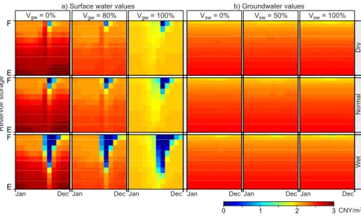
Figure 4.Temporal changes of the water values (CNY m−3)for the climate period before 1980. The marginal water value is the true value of storing a unit volume of water for later use and varies with reservoir storage levels, runoff flow class, and time of the year.(a)Surface water values at fixed [0, 80, 100 %] groundwater aquifer storage.(b)Groundwater values at fixed [0, 50, 100 %] surface water reservoir storage. The reservoir storage is shown fromE(empty) toF(full).
sample of the resulting equilibrium water value tables is pre-sented in Fig. 4. This figure shows the temporal variations of water values as a function of one state variable, keeping the other state variables at a fixed value. The state variables are fixed at empty, half full, and full storage respectively. Dur-ing the rainy season from June to August, high precipitation rates reduce water scarcity, resulting in lower surface water values. Because the groundwater storage capacity is much larger, increased recharge can easily be stored for later use, and groundwater values are therefore not affected. Addition of stream–aquifer interactions to the model is expected to af-fect this behavior, but since the flow in rivers/canals in the case study area is small most of the year, and since most areas are far from a river, it is reasonable to ignore these dynam-ics. The water values after 1980 are clearly higher than in the period before 1980 due to increased water scarcity caused by a reduction in the regional precipitation. In contrast, the groundwater value tables are uniform, with variation only in groundwater storage. The detailed water value tables are in-cluded in the Supplement.
We simulate management using the equilibrium water value tables as a pricing policy and force the system with 51 years of simulated historical runoff. Time series of the simulated groundwater storage can be seen in Fig. 5 for dif-ferent initial storage scenarios. The groundwater aquifer ap-proaches an equilibrium storage level around 260 km3(95 % full). If the storage in the aquifer is below this level, the av-erage recharge will exceed avav-erage pumping until the librium storage is reached. If the storage level is above equi-librium, average pumping will exceed average recharge un-til equilibrium is reached. In Fig. 6, the surface water and
1960 1970
Groundwater storage, km
3
1980
V0 = 200 km 3
V0 = 100 km 3
V0 = 0 km 3
1990 2000 0
50 100 150 200 250
Vmax,gw
Equilibrium storage
SDP DP EFC = 0
Figure 5.Simulated groundwater aquifer storage levels for 51 years of historical runoff with different initial groundwater tables (0, 100, 200, 258, and 275 km3). Results for the business-as-usual scenario (EFC is disregarded) and a benchmark scenario with perfect fore-sight (DP) are also shown.
groundwater storages are shown for a situation with equilib-rium groundwater storage. In most years, the surface water storage falls below 1 km3, leaving space in the reservoir for the rainy season. The potential high scarcity cost of facing a dry scenario with an almost empty reservoir is avoided by pumping more groundwater. These additional pumping costs seem to be exceeded by the benefits of minimizing spills in the rainy season. To demonstrate the business-as-usual solu-tion, the simulation model is run for a 20-year period with the present water demands and curtailment costs and with a discount rate set to infinity (i.e., zero future costs). The result-ing groundwater table is continuously decreasresult-ing, as shown in Fig. 5.
1970
Surface water storage, km
3
1980 1990 2000
0 1 2 3 4
V
max,sw
Groundwater storage, km
3
259 260 261 262 263
Groundwater Surface water
Figure 6.Simulated storage levels in the surface water reservoir and the groundwater aquifer at equilibrium groundwater storage.
PSW, M1
PGW, M1
PSW, M2
PGW, M2
PSW, M1
PGW, M1
PSW, M2
PGW, M2
1986 1988 1990 1992
1964 1966
User’s price, CNY/m
3
1968 1970
0 0.5 1.0 1.5 2.0 2.5
3.0 Initial groundwater storage at equilibrium (258 km3)
Initial groundwater storage below equilibrium (100 km3)
1986 1988 1990 1992
1964 1966
User’s price, CNY/m
3
1968 1970
0 0.5 1.0 1.5 2.0 2.5 3.0
Figure 7.User’s price for groundwater and surface water through for a 51-year simulation based on simulated historical runoff for two initial groundwater storages.P refers to the user’s price. M1 denotes results for a single surface water reservoir with a constant groundwater cost (Davidsen et al., 2015). M2 denotes results from the presented model framework with an additional dynamic groundwater aquifer. The user’s price for groundwater in M2 is the immediate pumping cost added to the marginal cost from the water value tables.
user’s price, which can be applied in a marginal cost pric-ing (MCP) scheme, is the marginal value of the last unit of water allocated to the users. The user’s price is the sum of the actual pumping cost (electricity used) and the additional marginal cost given by the equilibrium water value tables. In Fig. 7, the user’s prices for groundwater and surface water are shown for the 51-year simulation at and below the long-term sustainable groundwater storage level. When the groundwa-ter storage level is close to equilibrium, the user’s prices of groundwater and surface water are equal during periods with
0
50
0 100 150
20 40
W
a
ter allocations, % of demand
Time, months with water demand > 0
Uniform drawdown Uniform + stationary Thiem drawdown
60 80 100
50
0 100 150
Curtailment Surface water Groundwater
Figure 8.Composition of allocations and curtailments to wheat agriculture in the Hebei province for the months March, April, May, and June through 51-year simulation from an initial groundwater storage at equilibrium (258 km3). The results are shown for a simple drawdown model with uniform regional lowering of the groundwater table, and a more realistic drawdown model, which includes the stationary Thiem local drawdown cones.
CNY 3 m−3(see Fig. 7). As the aquifer slowly recovers, the
groundwater price decreases gradually.
At the equilibrium groundwater storage level, the user’s prices for groundwater is stable at around CNY 2.15 m−3, as
shown in Fig. 7. This indicates curtailment of wheat agri-culture in the downstream Hebei province, which has a will-ingness to pay CNY 2.12 m−3(see Table 1). The allocation
pattern to this user is shown in Fig. 8; the model switches between high curtailment and high allocations, depending on water availability and storage in the reservoirs. Groundwater allocations fluctuate between satisfying 0 and 80 % of the de-mand. Inclusion of the steady-state Thiem drawdown cones in the optimization model increases the marginal groundwa-ter pumping cost with increased pumping rates. Groundwa-ter allocations are distributed more evenly over the months, which results in less local drawdown. The total curtailments remain constant, while 1 % of the total water abstraction is shifted from groundwater to surface water, if the stationary Thiem drawdown is included. Inclusion of well drawdown significantly changed the simulated management but resulted in an only slightly increased computation time.
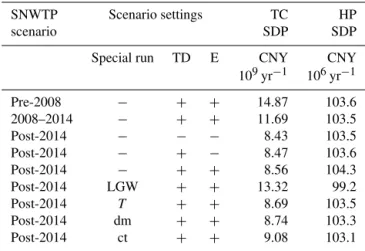
The average total costs of the 51-year simulation for dif-ferent scenarios can be seen in Table 3. The average reduc-tion in the total costs, associated with the introducreduc-tion of the SNWTP canal, can be used to estimate the expected marginal economic impact of the SNWTP water. The minimum total costs after the SNWTP is put in operation are compared to the scenario without the SNWTP (pre-2008) and divided by the allocated SNWTP water. The resulting marginal value of the SNWTP water delivered from Shijiazhuang to Beijing (2008–2014 scenario) is CNY 3.2 m−3, while the SNWTP
water from Yangtze River (post-2014 scenario) reduces the total costs with CNY 4.9 m−3. Similarly, a comparison of the
total costs for the post-2014 scenarios shows a marginal in-crease of CNY 0.91 m−3as a consequence of introducing a
minimum in-stream flow constraint.
Table 3.Average minimum total cost (TC) and hydropower benefits (HP) over the 51-year planning period for different scenario runs. SNWTP scenarios: pre-2008 refers to the period before the cen-tral route of the SNWTP was built; 2008–2014 refers to a situation with a partly completed SNWTP central route from Shijiazhuang to Beijing; post-2014 refers to the fully operational SNWTP cen-tral route from the Yangtze River to Beijing. Scenarios: LGW is initial groundwater storage at 100 km3(all other scenarios are initi-ated at equilibrium groundwater storage); dm is 10 % higher water demands; ct is 10 % higher curtailment costs ;T is 10 % higher transmissivity; TD is Thiem steady-state drawdown;Eis minimum ecosystem flow constraint; “+” is active and “−” is inactive.
SNWTP Scenario settings TC HP
scenario SDP SDP
Special run TD E CNY CNY
109yr−1 106yr−1
Pre-2008 − + + 14.87 103.6
2008–2014 − + + 11.69 103.5
Post-2014 − − − 8.43 103.5
Post-2014 − + − 8.47 103.6
Post-2014 − + + 8.56 104.3
Post-2014 LGW + + 13.32 99.2
Post-2014 T + + 8.69 103.5
Post-2014 dm + + 8.74 103.3
Post-2014 ct + + 9.08 103.1
CNY 8.46×10⁹yr−1. This is 1.3 % lower than the
equiva-lent SDP run (CNY 8.56×10⁹yr−1).
The minimum total costs were lowered from CNY 10.50×10⁹yr−1 (Davidsen et al., 2015) to
CNY 8.56×10⁹yr−1 (18 % reduction) by allowing the
groundwater aquifer to be utilized as buffer instead of a fixed monthly volume. This difference highlights the problem of defining realistic boundaries of optimization problems and shows that simple hard constraints, here fixed groundwater pumping limits, can highly limit the optimal decision space. With a dynamic groundwater aquifer, the model can mitigate dry periods and stabilize the user’s price of surface water as shown in Fig. 7. Finally, policies like minimum in-stream ecosystem flow constraints can be satisfied with less impact on users with high curtailment costs. The total costs without restrictions on the groundwater pumping have been esti-mated to be CNY 2.98×10⁹,yr−1 (Davidsen et al., 2015).
To end the groundwater overdraft in the basin, the present study thus estimates a cost increase of CNY 5.58×10⁹yr−1,
once the groundwater aquifer is at equilibrium storage. The cost of recharging the aquifer from the present storage level below the equilibrium is significantly higher. In Table 3, the LGW scenario shows that the average cost of sustainable management from an initial storage at 100 km3 (one-third full) is CNY 13.32×10⁹yr−1.
From any initial groundwater reservoir storage level, the model brings the groundwater table to an equilibrium stor-age level at approximately 95 % of the aquifer storstor-age capac-ity. Only small variations in the aquifer storage level are ob-served after the storage level reaches equilibrium as shown in Fig. 6. While addition of the Thiem stationary drawdown has only a small effect on total costs and total allocated water, it is clear from Fig. 8 that the additional Thiem drawdown highly impacts the allocation pattern for some of the water users. High groundwater pumping rates result in larger local drawdown and thus in higher pumping costs. This mecha-nism leads to a more uniform groundwater pumping strategy, which is clearly seen in Fig. 8, and results in a much more re-alistic management policy.
4 Discussion
This study presents a hydroeconomic optimization approach that provides a macroscale economic pricing policy in terms of water values for conjunctive surface water–groundwater management. The method was used to demonstrate how the water resources in the Ziya River basin should be priced over time, to reach a sustainable situation at minimum cost. We believe that the presented modeling framework has great po-tential use as a robust decision support tool in real-time water management. However, a number of limitations and simpli-fications need to be discussed.
A first limitation of the approach is the high level of sim-plification needed. There are two main reasons for the high level of simplification: limited data availability and the
lim-itations of the SDP method. The curse of dimensionality limits the approach to 2–3 interlinked storage facilities and higher dimensional management problems will not be com-putationally feasible with SDP today. This limit on the num-ber of surface water reservoirs and groundwater aquifers re-quires a strongly simplified representation of the real-world situation in the optimization model. The simulation phase following the optimization is not limited to the same ex-tent, since only a single subproblem is solved at each stage. The water values determined by the SDP scheme can thus be used to simulate management using a much more spatially resolved model with a high number of users; this was not demonstrated in this study. The advantage of SDP is that it provides a complete set of pricing policies that can be ap-plied in adaptive management, provided that the system can be simplified to a computationally feasible level. An alter-native approach known as stochastic dual dynamic program-ming (SDDP, Pereira and Pinto, 1991; Pereira et al., 1998) has shown great potential for multi-reservoir river basin wa-ter management problems. Instead of sampling the entire de-cision space with the same accuracy level, SDDP samples with a variable accuracy not predefined in a grid, focusing the highest accuracy around the optimal solution. This vari-able accuracy makes SDDP less suitvari-able for adaptive man-agement. Despite the highly simplified system representa-tion, we believe that the modeling framework provides inter-esting and nontrivial insights, which are extremely valuable for water resources management on the NCP.
Computation time was a limitation in this study. Three factors increased the computational load of the optimization model. (1) Inclusion of the groundwater state variable re-sulted in an exponential growth of the number of subprob-lems; (2) the non-convexity handled by the slower GA–LP formulation caused an increase in the computation time of 10–100 times a single LP; and (3) the SDP algorithm needed to run through more than 200 years to reach a steady state. A single scenario run required 4000 CPU hours and was solved in 2 weeks, using 12 cores at the high-performance comput-ing facilities at the Technical University of Denmark. This is 50 000 times more CPU hours than a single-reservoir SDP model (Davidsen et al., 2015). Since the water value tables can be used offline in the decision making, this long compu-tation time can be accepted.
generalized estimates of pumping cost, and a lumped ground-water model, which all contribute to the uncertainty. Further, poor data availability for the case study area required some rough estimates of the natural water availability, single-point demand curves, and perfect correlation between rainfall and groundwater recharge. The method-driven assumptions gen-erally limit the decision support to the basin scale, while the simple estimates caused by poor data availability contribute to raising the general uncertainty of the model results. Given the computational challenges and the diverse and significant uncertainties, the model results should be seen as a demon-stration of the model’s capabilities rather than precise cost estimates. Better estimates will require access to a more com-prehensive case data set and involve a complete sensitivity analysis.
Intuitively, one would expect the equilibrium groundwater storage level to be as close as possible to full capacity, while still ensuring that any incoming groundwater recharge can be stored. Finding the exact equilibrium groundwater storage level would require a very fine storage discretization, which, given the size of the groundwater storage, is computation-ally infeasible. Therefore the equilibrium groundwater stor-age level is subject to significant discretization errors. The long time steps (monthly) make the stationarity required for using the Thiem stationary drawdown method a realistic as-sumption.
The difference between total cost with SDP and with DP (perfect foresight) is small (1.3 %). Apart from Bei-jing, which has access to the SNWTP water, the remaining downstream users have unlimited access to groundwater. The large downstream groundwater aquifer serves as a buffer to the system and eliminates the economic consequences of a wrong decision. The model almost empties the reservoir ev-ery year as shown in Fig. 6, and wrong decisions are not punished with curtailment of expensive users as observed by Davidsen et al. (2015). The groundwater aquifer reduces the effect of wrong decisions by allowing the model to mini-mize spills from the reservoir without significant economic impact of facing a dry period with an empty reservoir. A dy-namic groundwater aquifer thereby makes the decision sup-port more robust, since it is the timing and not the amount of curtailment that is being affected.
The derived equilibrium groundwater value tables in Fig. 4 (and detailed water value tables in the Supplement) show that the groundwater values vary with groundwater storage alone and are independent of time of the year, the inflow and recharge scenario, and the storage in the surface water reser-voir. This finding is important for future work, as a substi-tution of the groundwater values with a simpler cost func-tion could greatly reduce the number of states and thereby the computation time. The equilibrium groundwater price, i.e., the groundwater values around the long-term equilib-rium groundwater storage, can possibly be estimated from the total renewable water and the water demands ahead of the optimization, but further work is required to test this.
Further work should also address the effect of discounting of the future costs on the equilibrium water value tables and the long-term steady-state groundwater table. In the present model setup, the large groundwater aquifer storage capacity forces the backward-moving SDP algorithm to run through 200–250 model years, until the water values converge to the long-term equilibrium. Another great improvement, given the availability of the required data, would be to replace the constant water demands with elastic demand curves in the highly flexible GA–LP setup.
A significant impact of including groundwater as a dy-namic aquifer is the more stable user’s prices shown in Fig. 7. The user’s price of groundwater consists of two parts: the im-mediate groundwater pumping costs (electricity costs) and the expected future costs represented by the groundwater value for the last allocated unit of water. As the model is run to equilibrium, the user’s prices converge towards the long-term equilibrium at approximately CNY 2.2 m−3. The
electricity price can be used as a policy tool to internalize the user’s prices of groundwater shown in Fig. 7. Stable water user’s prices will ease the implementation of, e.g., an MCP scheme, which is one of the available policy options to en-force long-term sustainability of groundwater management. 5 Conclusions
model is used to derive a pricing policy to bring the over-exploited groundwater aquifer back to a long-term sustain-able state. The economic efficient recovery policy is found by trading off the immediate costs of water scarcity with the long-term additional costs of a large groundwater head. From an initial storage at one-third of the aquifer capacity, the av-erage costs of ending groundwater overdraft are estimated to be CNY 13.32×10⁹yr−1. The long-term cost-effective
reservoir policy is to slowly recover the groundwater aquifer to a level close to the surface by gradually lowering the groundwater value from an initial level of CNY 3 m−3. Once
at this sustainable state, the groundwater values are almost constant at CNY 2.15 m−3, which suggests that wheat
agri-culture should generally be curtailed under periods of water scarcity. The dynamic groundwater aquifer serves as a buffer to the system and is used to bridge the water resources to multiple years. The average annual total costs are reduced by 18 % to CNY 8.56×10⁹yr−1compared to a simpler
formu-lation with fixed monthly pumping limits. The stable user’s prices are suitable to guide a policy scheme based on water prices, and the method has great potential as a basin-scale de-cision support tool in the context of the China No. 1 Policy Document.
The Supplement related to this article is available online at doi:10.5194/hess-20-771-2016-supplement.
Acknowledgements. S. Liu and X. Mo were supported by grants of the Natural Science Foundation of China (31171451, 41471026). The authors thank the numerous farmers and water managers in the Ziya River basin for sharing their experiences; L. S. Andersen from the China Europe Water Platform for sharing his strong willingness to assist with his expert insight on China; and K. N. Marker and L. B. Erlendsson for their extensive work on a related approach early in the development of the presented optimization framework.
Edited by: F. Pappenberger
References
Andreu, J., Capilla, J., and Sanchís, E.: AQUATOOL, a generalized decision-support system for water-resources planning and oper-ational management, J. Hydrol., 177, 269–291, 1996.
Bellman, R. E.: Dynamic Programming, Princeton University Press, Princeton, NJ, USA, 1957.
Berkoff, J.: China: The South-North Water Transfer Project – is it justified?, Water Policy, 5, 1–28, 2003.
Booker, J. F., Howitt, R. E., Michelsen, A. M., and Young, R. A.: Economics and the modeling of water resources and policies, Nat. Resour. Model., 25, 168–218, 2012.
Bright, E. A., Coleman, P. R., King, A. L., and Rose, A. N.: Land-Scan 2007, available at: http://web.ornl.gov/sci/landscan/ (last access: 15 February 2016), 2008.
Budyko, M.: The heat balance of the Earth’s surface, US Depart-ment of Commerce, Washington, USA, 1958.
Buras, N.: Conjunctive Operation of Dams and Aquifers, J. Hy-draul. Div., 89, 111–131, 1963.
Burt, O. R.: Optimal resource use over time with an application to ground water, Manage. Sci., 11, 80–93, 1964.
Cai, X., McKinney, D. C., and Lasdon, L. S.: Solving nonlinear water management models using a combined genetic algorithm and linear programming approach, Adv. Water Resour., 24, 667– 676, doi:10.1016/S0309-1708(00)00069-5, 2001.
CPC Central Committee and State Council: No. 1 Central Doc-ument for 2011, Decision from the CPC Central Commit-tee and the State Council on Accelerating Water Conservancy Reform and Development, available at: http://english.agri.gov. cn/hottopics/cpc/201301/t20130115_9544.htm (last access: 15 February 2016), 2010.
Davidsen, C., Pereira-Cardenal, S. J., Liu, S., Mo, X., Rosbjerg, D., and Bauer-Gottwein, P.: Using stochastic dynamic program-ming to support water resources management in the Ziya River basin, J. Water. Res. Pl.-ASCE, 141, 04014086-1–04014086-12, doi:10.1061/(ASCE)WR.1943-5452.0000482, 2015.
Deng, X.-P., Shan, L., Zhang, H., and Turner, N. C.: Im-proving agricultural water use efficiency in arid and semi-arid areas of China, Agr. Water Manage., 80, 23–40, doi:10.1016/j.agwat.2005.07.021, 2006.
Erlendsson, L. B.: Impacts of local drawdown on the optimal con-junctive use of groundwater and surface water resources in the Ziya River basin, China, Thesis, B.Sc. in engineering, Technical University of Denmark, Kgs. Lyngby, Denmark, 2014.
Goldberg, D. E.: Gentic Algorithms in Search, Optimization, and Machine Learning, Addison-Wesley Publishing Company, Inc., Boston, MA, USA, 1989.
Google Inc.: Google Earth, (version 7.1.2.2041), 2013.
Harou, J. J. and Lund, J. R.: Ending groundwater overdraft in hydrologic-economic systems, Hydrogeol. J., 16, 1039–1055, doi:10.1007/s10040-008-0300-7, 2008.
IBM: ILOG CPLEX Optimization Studio v. 12.4, 2013.
Ivanova, N.: Off the Deep End – Beijing’s Water Demand Out-paces Supply Despite Conservation, Recycling, and Imports, Circ. Blue, available at: http://www.circleofblue.org (last access: 15 February 2016), 2011.
Knapp, K. C. and Olson, L. J.: The Economics of Con-junctive Groundwater Management with Stochastic Sur-face Supplies, J. Environ. Econ. Manag., 28, 340–356, doi:10.1006/jeem.1995.1022, 1995.
Labadie, J.: Optimal operation of multireservoir systems: state-of-the-art review, J. Water Res. Pl.-ASCE, 130, 93–111, 2004. Lee, J.-H. and Labadie, J. W.: Stochastic optimization of
multireser-voir systems via reinforcement learning, Water Resour. Res., 43, W11408, doi:10.1029/2006WR005627, 2007.
Li, V.: Tiered power bill debated, Shenzhen Dly., 17 May, avail-able at: http://szdaily.sznews.com/html/2012-05/17/content_ 2046027.htm (last access: 15 February 2016), 2012.
Liu, C. and Xia, J.: Water problems and hydrological research in the Yellow River and the Huai and Hai River basins of China, Hydrol. Process., 18, 2197–2210, doi:10.1002/hyp.5524, 2004. Liu, C., Yu, J., and Kendy, E.: Groundwater Exploitation and Its
Loucks, D. P. and van Beek, E.: Water Resources Systems Planning and Management and Applications, UNESCO Publishing, Paris, France, 2005.
Maddock, T.: Algebraic technological function from a simulation model, Water Resour. Res., 8, 129–134, doi:10.1029/WR008i001p00129, 1972.
Marques, G. F., Lund, J. R., Leu, M. R., Jenkins, M., Howitt, R., Harter, T., Hatchett, S., Ruud, N., and Burke, S.: Econom-ically Driven Simulation of Regional Water Systems: Friant-Kern, California, J. Water. Res. Pl.-ASCE, 132, 468–479, doi:10.1061/(ASCE)0733-9496(2006)132:6(468), 2006. MathWorks Inc.: MATLAB (R2013a), v. 8.1.0.604, including the
Optimization Toolbox, Natick, MA, USA, 2013.
Mayne, D. Q., Rawlings, J. B., Rao, C. V., and Scokaert, P. O. M.: Constrained model predictive control: Stability and optimality, Automatica, 36, 789–814, doi:10.1016/S0005-1098(99)00214-9, 2000.
McKinney, D. C. and Lin, M.-D.: Genetic algorithm solution of groundwater management models, Water Resour. Res., 30, 1897–1906, doi:10.1029/94WR00554, 1994.
Mo, H.: N. China drought triggers water disputes, Xinhua, 25 May 2006, available at: http://news.xinhuanet.com/english/2006-05/ 24/content_4595096.htm (last access: 15 February 2016), 2006. Moiwo, J. P., Yang, Y., Li, H., Han, S., and Hu, Y.: Comparison of
GRACE with in situ hydrological measurement data shows stor-age depletion in Hai River basin, Northern China, Water South Africa, 35, 663–670, 2010.
Morari, M. and Lee, J. H.: Model predictive control?: past, present and future, Comput. Chem. Eng., 23, 667–682, 1999.
National Bureau of Statistics of China: Statistical Yearbook of the Republic of China 2011, The Chinese Statistical Associa-tion, available at: http://www.stats.gov.cn/tjsj/ndsj/2011/indexeh. htm (last access: 15 February 2016), 2011.
NGCC: Shapefile with provincial boundaries in China, Natl. Geo-matics Cent. China, 1 Baishengcun, Zizhuyuan, Beijing, China, 100044, 2009.
Nicklow, J., Reed, P., Savic, D., Dessalegne, T., Harrell, L., Chan-Hilton, A., Karamouz, M., Minsker, B., Ostfeld, A., Singh, A., and Zechman, E.: State of the Art for Genetic Algorithms and Beyond in Water Resources Planning and Management, J. Water. Res. Pl.-ASCE, 136, 412–432, doi:10.1061/(ASCE)WR.1943-5452.0000053, 2010.
Noel, J. E. and Howitt, R. E.: Conjunctive multibasin management: An optimal control approach, Water Resour. Res., 18, 753–763, doi:10.1029/WR018i004p00753, 1982.
Pereira, M., Campodónico, N., and Kelman, R.: Long-term Hydro Scheduling based on Stochastic Models, EPSOM’98, Zurich, 1– 22, available at: http://www.psr-inc.com/psr/download/papers/ pereira_epsom98.pdf (last access: 15 February 2016), 1998. Pereira, M. V. F. and Pinto, L. M. V. G.: Multi-stage stochastic
op-timization applied to energy planning, Math. Program., 52, 359– 375, 1991.
Philbrick, C. R. and Kitanidis, P. K.: Optimal conjunctive-use operations and plans, Water Resour. Res., 34, 1307–1316, doi:10.1029/98WR00258, 1998.
Provencher, B. and Burt, O.: Approximating the optimal ground-water pumping policy in a multiaquifer stochastic con-junctive use setting, Water Resour. Res., 30, 833–843, doi:10.1029/93WR02683, 1994.
Pulido-Velázquez, M., Andreu, J., and Sahuquillo, A.: Economic optimization of conjunctive use of surface water and groundwa-ter at the basin scale, J. Wagroundwa-ter. Res. Pl.-ASCE, 132, 454–467, 2006.
Qin, H., Cao, G., Kristensen, M., Refsgaard, J. C., Rasmussen, M. O., He, X., Liu, J., Shu, Y., and Zheng, C.: Integrated hydrologi-cal modeling of the North China Plain and implications for sus-tainable water management, Hydrol. Earth Syst. Sci., 17, 3759– 3778, doi:10.5194/hess-17-3759-2013, 2013.
Reeves, C. R.: Feature Article – Genetic Algorithms for the Operations Researcher, INFORMS J. Comput., 9, 231–250, doi:10.1287/ijoc.9.3.231, 1997.
Reichard, E. G.: Groundwater–Surface Water Management With Stochastic Surface Water Supplies: A Simulation Opti-mization Approach, Water Resour. Res., 31, 2845–2865, doi:10.1029/95WR02328, 1995.
Riegels, N., Pulido-Velazquez, M., Doulgeris, C., Sturm, V., Jensen, R., Møller, F., and Bauer-Gottwein, P.: Systems Analysis Ap-proach to the Design of Efficient Water Pricing Policies under the EU Water Framework Directive, J. Water. Res. Pl.-ASCE, 139, 574–582, doi:10.1061/(ASCE)WR.1943-5452.0000284, 2013. Saad, M. and Turgeon, A.: Application of principal component
anal-ysis to long-term reservoir management, Water Resour. Res., 24, 907–912, doi:10.1029/WR024i007p00907, 1988.
Siegfried, T. and Kinzelbach, W.: A multiobjective discrete stochastic optimization approach to shared aquifer management: Methodology and application, Water Resour. Res., 42, W02402, doi:10.1029/2005WR004321, 2006.
Siegfried, T., Bleuler, S., Laumanns, M., Zitzler, E., and Kinzel-bach, W.: Multiobjective Groundwater Management Using Evo-lutionary Algorithms, IEEE Trans. Evolut. Comput., 13, 229– 242, doi:10.1109/TEVC.2008.923391, 2009.
Singh, A.: Simulation–optimization modeling for conjunctive water use management, Agr. Water Manage., 141, 23–29, doi:10.1016/j.agwat.2014.04.003, 2014.
Stage, S. and Larsson, Y.: Incremental Cost of Water Power, Power Appar. Syst. Part III, Transactions Am. Inst. Electr. Eng., 80, 361–364, 1961.
Stedinger, J. R., Sule, B. F., and Loucks, D. P.: Stochastic dynamic programming models for reservoir operation optimization, Water Resour. Res., 20, 1499–1505, doi:10.1029/WR020i011p01499, 1984.
The People’s Government of Hebei Province: Water diver-sion project will benefit 500 million people, available at: http://www.chinadaily.com.cn/china/2012-12/27/content_ 16062623.htm (last access: 15 February 2016), 2012.
Thiem, G.: Hydrologische Methoden, Gebhardt, Leipzig, Germany, 56, 1906.
Tsur, Y.: The stabilization role of groundwater when sur-face water supplies are uncertain: The implications for groundwater development, Water Resour. Res., 26, 811–818, doi:10.1029/WR026i005p00811, 1990.
Tsur, Y. and Graham-Tomasi, T.: The buffer value of groundwater with stochastic surface water supplies, J. Environ. Econ. Manag., 21, 201–224, doi:10.1016/0095-0696(91)90027-G, 1991. USDA Foreign Agricultural Service: Grain and Feed Annual 2012,
USGS: Shuttle Radar Topography Mission, 1 Arc Second scenes, Unfilled Unfinished 2.0, Univ. Maryland, College Park, MD, USA, 2004.
USGS: Eurasia land cover characteristics database version 2.0, USGS land use/land cover scheme, United States Geologi-cal Survey, available at: http://edc2.usgs.gov/glcc/tablambert_ euras_as.php, 2013.
Wang, B., Jin, M., Nimmo, J. R., Yang, L., and Wang, W.: Estimat-ing groundwater recharge in Hebei Plain, China under varyEstimat-ing land use practices using tritium and bromide tracers, J. Hydrol., 356, 209–222, doi:10.1016/j.jhydrol.2008.04.011, 2008. World Bank: Agenda for Water Sector Strategy for North China,
Volume 2, Main Report, Report No. 22040-CHA CHINA, avail-able at: http://documents.worldbank.org/, 2001.
Yang, C.-C., Chang, L.-C., Chen, C.-S., and Yeh, M.-S.: Multi-objective Planning for Conjunctive Use of Surface and Subsur-face Water Using Genetic Algorithm and Dynamics Program-ming, Water Resour. Manag., 23, 417–437, doi:10.1007/s11269-008-9281-5, 2008.
Yu, H.: Shanxi to raise electricity price, Chinadaily, available at: http://www.chinadaily.com.cn/business/2011-04/15/content_ 12335703.htm (last access: 15 February 2016), 2011.
Zhang, L., Potter, N., Hickel, K., Zhang, Y., and Shao, Q.: Wa-ter balance modeling over variable time scales based on the Budyko framework–Model development and testing, J. Hydrol., 360, 117–131, doi:10.1016/j.jhydrol.2008.07.021, 2008. Zheng, C., Liu, J., Cao, G., Kendy, E., Wang, H., and Jia, Y.: Can