Old-age benefits and retirement decisions of rural elderly in Brazil

(1)

E:lretirementO 1-120202.doc

OLD-AGE BENEFITS AND RETIREMENT DECISIONS OF

RURAL ELDERL Y IN BRAZIL

a

Irineu Evangelista de Carvalho Filhob

First version: June 1999 - This version: December 1, 2002

Abstract:

I estimate the impact of social security benefits on retirement decisions of rural workers by studying changes in the roles governing social security in Brazil. I focus on a 1991 reform, which brought a reduction in the minimum eligibility age for males and females, a doubling of benefit values and the extension of benefits to non-heads of households. Because beneficiaries are not subject to means or retirement tests, I estimate apure income effect. I find that a reduction in the minimum eligibility age for old-age benefits was an important determinant in the reduction in labor supply of elderly rural workers in Brazil. Finally, I find that benefit take-up rates are larger among the better educated, but least-schooled workers show the largest labor supply responses to the reformo

a This paper is an adaptation of Chapter 1 of my Ph.D. Thesis. FinanciaI support from CNPq, the National Institute of Aging, the Center for Retirement Research at Boston College and the Schultz Fund at MIT is thankfully acknowledged. I am grateful to my advisors Josh Angrist, Daron Acemoglu, Abhijit BaneIjee, Dora Costa and Esther Duflo for their comments at different stages of this paper. Special thanks go to Dora Costa for crucial support during ali stages of this project. Marcos Chamon in particular and participants at the MIT LaborlPublic Finance Seminar and Labor, Development Economics and Econometrics lunches and Georgetown University and Bowdoin College seminars also deserve thanks for their inputs to this project. Errors are mine.

(2)

Population estimates by the United Nations indicate that 56% of the world's 65 and over population lived in developing countries in 1990.1 Moreover, the elderly proportion share of the population is increasing in most developing countries, due to gains in longevity. The aging of developing countries' populations raises concems about the living conditions of their elderly, especially in countries where incipient development has already weakened traditional family links or strong filial piety motives are not emphasized. With the aging of developing countries' populations, social security arrangements may be called for where they are not already in place.

The introduction or expansion of transfer programs for the elderly has several consequences on the labor market equilibrium. Perhaps the most salient of them are changes in the labor supply pattems of the elderly. The challenge for policymakers is to design systems that do not create excessive burden on workers and employers, particularly social security systems that do not generate too large an impact on the labor supply ofthe elderly and dependency ratios.

Because developing countries differ from developed countries in a variety of ways, the accumulated knowledge from studies of social security based on developed countries might be of limited relevance.2 Moreover, there are only few studies about retirement decisions in developing countries. 3

(3)

Factors such as small asset holdings, low lifetime income, poorer health and likely poor access to leisure opportunities suggest that working as long as one's body permits may be the more common strategy among the rural elderly in developing countries.

On the other hand, low capital intensity in rural activities may cause work to be particularly arduous and degrading for elderly people. Previous evidence from developed countries suggests that income effects for low-income are larger than income effects for high-income workers.4 Evidence from developed countries suggests that relatively few workers retire before they become eligible for social security (Kahn 1988; Johnson 1999), perhaps because of credit constraints. Because the development of the financiaI sector is positively correlated with income leveIs (Levine 1997), the connection between the minimum eligibility age to benefits and the usual retirement age might be stronger in developing countries.

The Brazilian social security reform of 1991 reduced the minimum eligibility age for rural old-age benefits for men from 65 to 60, increased the minimum benefit paid to rural old-age beneficiaries from 50% to 100% of the minimum wage, extended old-age benefits to female rural workers who were not heads of households, and reduced the age at which women qualified for benefits from 65 to 55. This reform provides a unique opportunity to study the effect of benefits on retirement in developing countries for three reasons.

(4)

Second, because eligibility for rural benefits depends only on predetennined characteristics of workers and there are no means or retirement tests, the effects of increases in benefits or extension of eligibility in this program generates apure income effect.

Third, the structure of the refonn allows for the use of instrumental variables for income from benefits, in a way that address problems such as measurement errors in the benefits variable (relevant in a high inflation country) and omitted variables bias.

In this paper, I am able to use changes in rules goveming eligibility and benefit values in the old-age program for rural workers to identify the effect of old-age benefits on male elderly labor supply. These changes in rules and benefit values provi de me with an exogenous source of variation in benefits that is not correlated with a worker's idiosyncratic preferences for work. I first use a differences-in-differences-in-differences (triple differences) approach, where I compare changes in benefit take-up rates and labor variables for rural and urban workers of different age groups. Then, I move to structural estimation of the parameter of interest. The gradual build-up of benefit take-up rates, the change in the minimum eligibility age, the differential increase in benefits for rural workers, and the rule changes affecting female workers all provide me with a set of instrumental variables capturing exogenous variation in social security benefits. In addition, because benefit take-up rates may be correlated with factors that enhance labor market perfonnance, such as ability or education, I analyze the differences in take-up rates and labor supply responses across education groups.

(5)

R$100 increase in benefits increases the probability that workers "did not work in the reference week" by 15.0 percentage points; receipt of benefits increases the same probability by 45.2 percentage points. Those estimates imply elasticities of labor force non-participation with respect to benefit values and to benefit receipt equal to 0.65 and 0.70 respectively - a large figure compared to the evidence from developed countries (e.g. Krueger and Pischke (1992». I also find that benefit take-up rates are larger among the better educated, but that least-schooled workers change their labor supply the mosto

Section 1 summarizes the reform, describes the data, our outcomes of interest and sample selection choices. Section 2 presents the identification strategy; triple differences estimates using age. time and occupation variation; and presents graphs that summarize the evidence on the first-stage relationship. Section 3 presents triple difference estimates for benefit take-up rates and labor responses. Section 4 presents instrumental variables estimates of the effect of benefits on labor supply and how they differ across different educational groups. Section 5 concludes discussing the results and their implications for policy.

1.

The 1991 Reform in the Brazilian Social Security System

(6)

Male rural workers were affected by: (l) a reduction in the minimum eligibility age from 65 to 60; (2) an increase in benefits from 50% to 100% of a minimum wage; and, (3) extension of access to length-of-service benefits (see Table 1). Female rural workers were affected by: (1) a reduction in the minimum eligibility age from 65 to 55; and, (2) the end of the one person-per-household restriction, which allowed married females to take-up benefits too.

The refonn went into effect when the necessary Ordinary Law was passed in July 24, 1991 (Lei #8212/8213). After that, the increase in the value of outstanding benefits went automaticalIy into effect, but actual extension ofbenefits to newly eligible workers took a few months to be processed for a variety ofreasons (administrative delay, distance to the nearest post office, lack ofinfonnation about entitlements and others).

(7)

eligible males aged 60-64 were receiving rural old age benefits; by the end of 1993, 326,158 were; by the end of 1994 that figure was 358,761.

The last year before the Constitutional change was passed for which the survey data is available is 1987. Data is available also for 1988 and 1989. The latest year before the actual implementation ofthe reform for which data is available is 1990. There are no data for 1991. In 1992, old-age benefits have already increased and take-up of new benefits is still partial, which allows us to take advantage of additional time variation in take-up rates. In 1993, the take-up process is almost "complete". There are no data for 1994. The earliest year after the take-up process has been "completed" for which data is available is 1995.

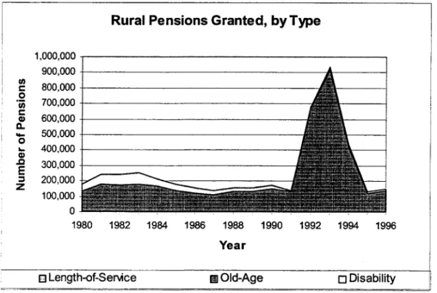
The reform described above provides exogenous variation in social security benefits, which will be used to estimate the effect of those benefits on labor supply. Figure 1 shows the time series of the flow of new pension benefits. Although the change in the law happened in July 1991, there does not seem be any increase in the flow of granted benefits per year before 1992. The spike in the number of granted old-age benefits lasted until 1994 (Anuário Estatístico da Previdência (1998)). The yearly amount of new disability benefits shrinks after the reform implementation, suggesting that disability and old-age benefits are substitutes for the age group affected by the reformo The number of granted rural length-of-service benefits is only about 0.5% of all rural benefits and is hardly visible in the picture. Therefore, the impact ofthe extension of access to length-of-service pensions is likely to be small or negligible.

(8)

wage. Therefore, rural workers had no incentive to postpone their application to benefits. Since the reform, the same formula for calculation of urban workers' benefits applies, which is a function of documented past eamings. However, because the vast majority of rural workers do not have a long history of documented eamings, nearly 100% of rural beneficiaries are at the comer, receiving exactly the minimum benefit equal to 100% of the minimum wage. (Appendix Table 2 shows that the average old-age benefit in 1997 was R$121.37, while the minimum wage was R$120).

It is worthwhile noting that aposentadorias rurais (rural pensions) contain no incentives for total withdrawal from the labor force. There is no eamings test and, unlike their urban counterparts, rural workers do not have to quit their jobs to become eligible for benefits5. Therefore, examining only discrete measures oflabor supply (as is common for studies of retirement in the United States) might miss the adjustment in the intensity margin, captured by total hours.

(9)

The labor supply measures that 1 use should capture different features ofthe retirement decision in the population of interest. The basic binary indicator of retirement decision is the variable "did not work in the week ofreference". To explore the intensity ofwork, 1 use total hours per week.

Unfortunately, the data do not allow me to determine the type of social security benefits paid to each beneficiary. The PNAD classifies social security benefits into somewhat broad categories. It only differentiates between aposentadorias (disability, old age and length of service benefits) and pensões (military and survivors' income maintenance benefits). Pensões are mostly received by widows whose husbands were covered by social security benefits.

In my baseline specification, 1 identified rural and urban workers based on their occupations. I observe every worker's current occupation and 1 observe past occupation up to a four years recall.6 IndividuaIs who do not report their occupation or who have not worked in the last 4 years are classified as having ''undefined'' occupation. My results are not sensitive to the use of location of residence as a proxy for occupation for those workers whose occupation is undefined, or to the assignrnent of urban occupation for all workers with undefined occupation.7

(10)

restrict both the rural and urban samples to workers who had less than 12 years of schooling.

2. Identification

Strategy

I identify the effects of the refonn on labor supply by exploring a legislated exogenous variation over time in benefits availability, take-up rates and benefit values. The refonn of social security in question, passed in 1991, made male rural workers age 60-64 eligible to old-age benefits, while benefits paid out to alI eligible male rural workers - including the already eligible 65 years old or older - doubled.

Eligibility to rural benefits is based on age, occupational history and whether the observation pertains to the period before or after the refonn. I can therefore use this infonnation to infer benefit eligibility for each observation in the sample, fonned by a time series of cross-sections of a representative annual household survey.

The results in this paper will be presented first as triple differences estimates, without controlling for characteristics other than age, occupation and year of observation; then regression estimates with controls; then IV estimates where functions of age, occupation and year of observation are used as instruments for benefit receipt or benefit amount received.

2.1. Triple Differences Strategy

The comparison between changes in outcomes for a group affected by the refonn (treated group) and a group unaffected (control group) is at the heart of

(11)

labor force participation. Let the change in the outcomes of the treated group be LlLT or (LT,post - LT,pre). This change may be due to the changes in the social security rules those workers are facing, but also for other time specific factors that affect also the control group. If those time specific factors are additive, they can be "differenced away" with the subtraction of the change in outcomes for the control group, LlLc, from LlLT. The differences-in-differences estimate for the impact ofthe reform is DD = (L1Lr -L1Lc) =

(Luosl - LT.pre) - (LC,Posl - LC,pre). For instance, for the group aged 60-64, rural workers

were affected by the reform, whereas urban workers were noto Hence, comparing the outcome of interest changed differently across rural and urban workers would provide a differences-in-differences estimate.

The idea is to use the trend for the 'control group to construct a counterfactual to the reform for the treated group. The identification condition is that there is no shock to the relative labor market outcomes of the treatment and control groups contemporaneous to the reformo That may be a strong identification assumption, after alI, there are observable and unobservable differences between the treated and the control group that may account for relative shifts in the outcomes of interest.

Dne can control for different relative shocks that might have affected rural and urban

(12)

variables, but not due to the intervention. Hence, if subscripts A and U denote "affected"

and "unaffected", the triple-differences estimates are obtained from the subtraction ofthe

differences-in-differences estimates based on the "non-affected" pair from the

differences-in-differences estimates based on the "affected" pair, i.e.,

DDD = _{DDA -DDu}= (L1LT -L1Lc)A - (L1LT -L1Lc)u (1)

For instance, the age groups 55-59 and 65-69 were, if anything, less affected by the

refonn than the age group 60-64. The difference in changes in outcomes across rural and

urban workers aged 60-64 is the differences-in-differences for the "affected" group or

DDA• The difference in changes in outcomes across rural and urban workers aged 55-59

or 65-69 is the differences-in-differences for the "unaffected" group or DDu.

2.2. Regression Interpretation

Triple-differences estimates have a regression interpretation: triple differences

estimates can also be obtained as the coefficient on the interaction between AFTER,

RURAL and a durnmy for the affected age group, TREAT, afier controlling for the effects

of alI combinations between any two ofthe variables above.

For example:

Z = ag + _{a 1}z AFTER + a; RURAL + a; TREAT + f31Z (TREAT x RURAL) (2)

+ f3; (AFTERx TREAT) + f3; (RURAL x AFTER)

+ f3z (AFTER x RURAL x TREAT) + v

Y=ao +a1AFTER+a2RURAL+a3TREAT + f31 (TREATx RURAL) (3)

+ f32(AFTERxTREAT)+ f33 (RURAL x AFTER)

+ f3r(AFTER x RURAL x TREAT) + v

In equation (2), Z is the receipt of social security benefits. In (3), Y is the labor supply

(13)

fixed year effect, and TREAT is a dummy for the age group that was treated by the

program change (1 iftreatment group, O if control group). The coefficient 131 controls for secular differences between rural and urban male workers in the treated age group. The

coefficient 132 controls for the time trend specific to the age group (aged 60-64) affected

by the reformo The coefficient 133 controls for the time trend specific to alI rural workers.

The coefficient

I3z

(l3y) on the interaction of age, location, and year is the triple difference

estimate and identifies the impact of the reform on benefit receipt (labor supply). The

triple difference estimator has the interpretation of a reduced form estimate, capturing the

effect of the mIe change on the group means of the outcome variable. Moreover, the ratio

l3y/l3z is numerically equal to the instrumental variables estimate of the effect of benefit

receipt on labor supply when I use the triple interaction term as the instrument for the

benefit variable.

2.3. Instrumental Variables Strategy

The triple-differences estimates described in the previous sections are reduced form

estimates and do not control for other determinants beyond occupation, age and year

effects. The structural model I want to estimate is:

y =

l30wn

OwnBenefits + <\>J(age, occupation, time) + X Õ + '\) (4)

In the equation above, <1>1 denotes a full set of age, occupation, time, age-occupation, age-time and occupation-time effects and X is a set of other control variables.

The existence of correlation between v and the benefit variables, i.e., between the

heterogeneity in preferences towards labor force participation and the benefit variables,

(14)

One source for this bias may be differences in the actual access to benefits across workers with different leveIs of ability. To receive benefits, a worker has to establish his eligibility through a bureaucratic process that requires proofs of age, occupation and in some cases past contributions to the Social Security system. More able or more educated workers may have an advantage because they are more likely to work in the formal sector or more able to understand the roles of the game. In this case, if ability is positively correlated with preferences for work, then OLS estimates of the effect of benefits on labor supply will be biased downwards. If workers with less attachment to their labor force participation are the ones more involved in gathering information about benefits entitlements (or preemptively organizing the necessary documents), then it will be the case they will be the first ones in the queue for receiving newly granted benefits. In this case, the OLS bias will go in the opposite direction: it would generate an upward bias (in absolute terms) in the parameter that measures the effect of the benefit.

Measurement errors in benefit values are another source of bias in the OLS estimates. The Brazilian economy suffered from very high inflation rates during the period studied in this paper and this could have created confusion about the nominal values of benefits (readjusted monthly through part of this period) in a survey where respondents self-report the leveI and composition of their income.

(15)

of observed variables like occupation and age and variables not observed by the econometrician such as health status.

I constructed instruments for benefit values, which incorporate variation in age, time and occupation. The interaction between rural workers, age 60-64 and after-period will instrument for the increases in benefits accruing to the 60-64 rural males who became eligible to old-age benefits with the reformo To take into account the gradual character of the changes caused by the reform, this instrument can be interacted with an indicator for both years after the reform: 1992 and 1993. The interaction between rural workers, age 65 and up and after period will instrument for the increases in the value of old-age benefits from 50% to 100% of the minimum wage occurred in 1991 affecting old-age beneficiaries already in the benefit payroll.

3. Triple Differences: Results

3.1. Benefit Take-Up Rates

(16)

represented in the axes, along with standard errors of the means. The point estimates in Table 3 show that the change in aposentadorias benefit take-up rates for rural workers aged 60-64 ("affected" group) was 23.59 percentage points larger than that oftheir urban counterparts during the period immediately before and after the reformo The same statistic for the "unaffected" groups was only -0.91 percentage points for the 55-59 years old and 6.27 percentage points for the 65-69 years old, both statistically insignificant. Therefore, the triple differences in the aposentadorias benefit take-up rates of by the targeted group increased 24.50 (17.32) percentage points, when I use 55-59 (65-69) year-olds as the "unaffected" groUp.9

Table 4 presents similar estimates for average benefit receipts. Rural males aged 60-64 became eligible for old-age benefits with the reformo Between 1990 and 1993, their average benefits increased from R$12.72 to R$101.57 (in Reais of September of 1997). For the same age group, but with urban occupations, average benefits increased from R$91.00 to R$ 151.98, yielding average benefits for rural workers increased R$27.87 more than for urban workers during the period of study, not statistically different from zero. In the central panel ofTable 4, there are the estimates for the "unaffected" group of 55-59 years old, whose eligibility status did not change, showing a difference-in-differences of negative R$25.I3, statistically not different from zero. This ''unaffected'' 55-59 age group allows me to control for trends over time in benefits differentials between rural and urban areas. The difference between the two difference-in-differences estimates is the triple differences estimate equal to R$53.60, with a t-statistic of 1.59. In

(17)

Remember that the eligibility status of males age 65-69 did not change with the reform, but their old-age benefits, originally set equal to Yz minimum wage, increased to one minimum wage. This result suggests that despite the doubling of rural benefits measured in terms of the minimum wage, rural workers seem to have lagged behind urban workers in terms of changes in the leveI of their benefits. The implied triple difference estimates by comparing the 60-64 and 65-69 age groups is negative R$31.53, not statistically distinguishable from zero.

The triple differences estimates of the effect of the reform on the outcomes of interest can be made more precise with the inclusion of additional controls in a regression framework. Table 6 presents the coefficients on the interaction between rural occupation, post-reform dummies and affected age group in a regressiQn with controls age, rural/urban and year effects, and all second leveI interactions between those variables. I also present results for two sub-samples related to educationallevels: some schooling and no schooling. The estimates on column (l) of Table 6 imply that as a consequence of the reform, benefit take-up rates for rural males aged 60-64 rose gradually by 12.1 and 34.0 percentage points, respectively in 1992 and 1993, compared to a counterfactual with no reformo The estimates in columns (2)-(3) show that benefit take-up rates increased significantly faster and by a larger amount for elderly males with some schooling than for the ones with no schooling. The estimates of the effects of the reform on monthly benefits, reported on columns (4)-(6), show a qualitatively similar pattem of larger increases in monthly benefits for rural workers with some schooling.

(18)

information, are more likely to understand their rights and entitlements, and are more likely to have the necessary documentation.

3.2. Labor Force Effects

Table 5 presents the triple differences estimates for the variable "did not work week 01 relerence n. Those results are typical of all other labor supply outcomes we analyzed and will not report for brevity. The proportion of rural workers aged 60-64 who did not work in the week of reference increased statistically and economically significant 9.48 percentage points more than the figures for urban workers of the same age, during the period immediately before and after the reformo

This finding is likely caused by the reform in question, because for the ''unaffected'' groups, no such differential in behavior between rural and urban workers was found. The differences-in-differences estimates were statistically insignificant -1.28 and 2.88 percentage points respectively for the ''unaffected'' groups aged 55-59 and 65-69 years.

Therefore, triple-differences estimates imply that there was a statistically significant 10.76 or 6.60 percentage points increase in the proportion of rural workers aged 60-64 who "did not work in the week of reference", depending on the choice of the "unaffected" group.

The ratio of the triple difference estimates for the effect of the reform on "did not work in the week of reference" and the "benefit take-up rates" is consistent with an IV estimate of the marginal effect of benefit take-up rates on labor participation in the 30-40% range, depending on the "unaffected" group of choice.

3.3. Visual Interpretation

(19)

1984, long before the refonn was thought of; 1987, right before the Constitutional change; 1990, right before the passing of the ordinary law implementing the changes; 1992, right after the program starts; and 1993, when the refonn is likely to have full effects.

For rural area males, there is a remarkable increase in benefit take-up in 1992 and 1993 for the cohorts age 61 to 64, which can be observed in the top left graph of Figure 2. The age benefit take-up profiles for ali years before 1992 have a similar shape: there is a steep increase by age 65, the pre-refonn eligibility age for rural old-age benefits, and take-up rates approach 100% for the older old. The implementation of the refonns shifted the age at which a 50% male benefit take-up rate is achieved in the rural area from 65-66 to 61. For urban area males, age benefit up profiles show a smooth increase in take-up rates with age. which can be explained by a large proportion of urban workers receiving "length-of-service" benefits. The absence of a noticeable spike in the distribution of ages at which urban workers take up benefits can be explained by the accumulation of years of documented work at different rates, due to different unemployment and infonnal work spells and different ages of first entry at the labor force. More importantly for the identification strategy, there does not seem to be any remarkable change in the age benefit take-up profiles ofurban workers.

(20)

4. IV: Results

Table 7 reports the OLS and IV estimates of the coefficient of "benefit receiver" durnmy and "monthly benefits" leveIs on three labor outcomes: "did not work in the reference week", "total hours per week" and "monthly eamings".

I find that OLS estimates are in general smalIer in absolute value than IVestimates for alI dependent variables, and more so for monthly benefits. The difference between IV and OLS estimates in this case may be due to measurement error in the benefit variables and correlation between benefit values and preferences for work - but because this difference is wider for likely poorly measured monthly benefits, measurement error seems to play a central role.

Instrumental variables estimates imply that receipt of an "aposentadoria" benefit causes an increase in the probability of not working in the reference week of 45.2 percentage points, a reduction in the hours worked per week of 25.2 hours and a reduction of monthly eamings of -R$632. Workers with some schooling reduce their labor supply less than the ones with no schooling - e.g. their reduction in labor participation was 12.8 percentage points smalIer than for workers with no schooling. However the effects on monthly eamings are greater for workers with some schooling -after alI, workers with some schooling eam more per hour than the ones with no schooling.

Instrumental variables estimates confirm a similar pattem for the effects of monthly benefits: R$100 of benefits are found to increase the probability of not working in the reference week by 15.0 percentage points, to reduce hours worked per week by 8.5 hours,

(21)

and to reduce monthly eamings by -R$317. Differences across workers of different educationallevels show a larger participation and hours response among workers with no schooling and a larger monthly eamings reduction among the ones with some schooling.

Different labor responses to benefits across educational groups may have arisen for a variety of reasons: more educated workers may have access to more capital - which can make their tasks at work less physically demanding; also, for a given flat benefit, more educated workers will have lower replacement rates because they have greater eaming potential.

5. Conclusions

The reform in the Brazilian social security system in 1991 provides an opportunity to leam about labor supply responses to: reductions in the minimum eligibility age for old-age benefits, increases in benefit leveIs, and about how social programs reach groups with different education leveIs in developing countries.

This paper estimates apure income effect - the vast majority of the existing literature has estimated total effects that are the sum of an income and a substitution effect, the latter due to means, income, eamings or retirement tests. In the standard case of leisure as a normal good, the income and substitution effects of means tested uneamed income point to the same direction. All else being equal, one should expect smaller total effects in the program analyzed in this paper than if means testing were in place.

(22)

by the reform (elderly age 60-64) with the soon-to-be-eligible (elderly age 55-59), its estimates are likely an underestimate ofthe actual responses.

The results show that elderly rural workers in Brazil are more strongly responsive to benefit income than elderly workers in developed countries. Instrumental variables estimates suggest that each unit of monthly benefits displaces 3.1 units of earned income - despite the fact that that is apure income effect. The large estimate for the effect of current benefits on eamings can be explained by substitution of non-remunerated activities, such as subsistence agriculture, unpaid work and leisure, for wage earning and remunerated activities.11 Another factor explaining this remarkable sensitivity to benefit income might well be the smaller riskiness of benefit income relative to the typical income volatility of a rural worker in a developing country.

The main policy lesson from this paper is that govemments should proceed with caution in the implementation of social security programs or other distributive policies, taking into account the possibility of substantial output losses. Of course, this recommendation includes neither efficiency nor equity judgments, but on1y an observation about the costs likely to be incurred with the implementation of such programs. Furthermore, if labor markets are characterized by high unemployment or non-participation rates of the youths and those non-employed fill the vacancies open by the retired elderly, output losses due to retirement may be minimized. Evaluating the effect of this reform on the employment rates of youths is an interesting undertaking for future research.

(23)

understand the formal roles of the game or because they are better informed in general. Given that this program of rural pensions is widely viewed as a program very successful in targeting the poor (Filgueiras 1998), this result suggests that goverrunents in developing countries should put more effort into making their social programs as universal as possible. Otherwise, scarce resources will be spent, without really achieving the most basic equity goal: reaching for the ones that need the most.

BIBLIOGRAPHY

Barroso Leite, Celso, 1978. Social Security in Brazil, Intemational Social Security Review, 31,318-329.

Cardoso de Oliveira, M.V., 1961. Social Security in Brazil, Intemational Labor Review, 84, 376-393.

Carvalho, Irineu, 2000. Old-Age Benefits and the Labor Supply ofRural Elderly in Brazil - mimeo.

Case, Anne and Angus Deaton, 1998. Large Cash Transfers to the Elderly in South Africa, Economic Joumal; vol. 108 n450, pp. 1330-61.

Chiarelli, Carlos, 1976. Social Security for Rural Workers in Brazil, Intemational Labour Review; vl13 n2 March-ApriI1976, pp. 159-69.

Cook, T. D. and Campbell, D. T., 1979. Quasi-Experimentation: Design and Analysis Issues for Field Settings, Chicago: Rand McNally.

Delgado, Guilherme Costa et alli, 1999. A valiacao Socioeconômica e Regional da Previdência Social Rural- Fase 11, Relatório Parcial dos Primeiros Resultados para a Região Sul do Brasil, IPEA, Brasília.

Filgueiras, Otto, 1998. Os Credores do Brasil, Teoria e Debate n039 (nov/dec/jan 1998). Hausman, Jerry, 1985. Taxes and Labor Supply, Handbook ofPublic Economics, vol. 1,

ed. Alan Auerbach and Martin F eldstein.

(24)

Johnson, Richard, 1999. The Effect of Social Security on Male Retirement: Evidence from Historical Cross-Country Data, mimeo Harvard.

Krueger, Alan and Jõrn-Steffen Pischke, 1992. The Effect of Social Security on Labor Supply: A Cohort Analysis ofthe Notch Generation, Journal ofLabor Economics 10, no.4:412-37.

Levine, Ross, 1997. FinanciaI Development and Economic Growth: Views and Agenda, Journal ofEconomic Literature; v35 n2 June 1997, pp. 688-726.

Malloy, James M., 1979. The Politics of Social Security in Brazil, The University of Pittsburgh Press.

Mesa-Lago, Carmelo, 1989. Social Security in Latin America and the Caribbean: a Comparative Assessment, in Ahmad, Dreze, Hills and Sen, Social Security in Developing Countries, Clarendon Press.

Meyer, Bruce, 1995. Natural and Quasi-Experiments in Economics, Journal ofBusiness and Economics Statistics, April 1995, VoI. 13, No. 2.

Stock, James and David A. Wise, 1990. Pensions, the Option Value of Work, and Retirement, Econometrica 58(5): 1151-1180.

(25)

Table 1

Occupation Programs

Rural Workers Urban Workers Old-Age Length-of-Service Disability Old-Age Length-of-Service Disability

Characteristics of the Brazilian Social Security System Before and After the Reform

The System Defore the Reform

Eligibility at age 65+, rural work documented for I ofpast 3 years. Only I person per household is eligible.

Benefit is flat and equal to 50% ofthe minimum wage. No restriction on gainful work.

No bonus for deferment ofpension receipt. No need to quit the current job to apply for benefits. No eamings/retirement test after that

Not available for rural workers.

Available at any age. Needs to stop working altogether. Benefit is flat and equal to 50% ofthe minimum wage

Eligibility at age 70. Benefit is 90% ofminimum wage. Needs to quit the current job to apply for benefits. No eamings/retirement test after that

Eligibility after 30 years of dec\ared documented work. Full benefits after 35 years of documented work. Fewer years for some types ofwork.

No minimum age requirement.

Benefits determined by years of documented work and recent labor eamings. Generous benefits for public sector work.

Minimum benefit is 90% ofthe minimum wage

Bonus for continued work beyond maximum eligibility period. Needs to quit the current job to apply for benefits. No eamings/retirement test after that.

Available at any age. Needs to stop working altogether. Benefit is 90% ofminimum wage.

Changes with the Reform

Minimum age for eligibility reduced to 60 for males and 55 for females.

No restriction in the number ofreceivers in a household. Benefit is 70% of eamings-based benefit plus I % for each 12 past payment of the payroll tax, up to 100%. Minimum benefit is increased to 100% of the minimum wage.

Same rules as urban workers.

Benefit is 80% of eamings-based benefit plus I % for each 12 past payment ofthe payroll tax, up to 100%. Minimum benefit is increased to 100% of the minimum wage.

Benefit is 70% of eamings-based benefit plus I % for each 12 past payment ofthe payroll tax, up to 100%.

Minimum benefit increased to 100% ofthe minimum wage.

Minimum eligibility for females reduced to 25 years of service. Benefit is 70% of eamings-based benefit at the minimum eligibility age plus 6% for each additional year of service beyond it, up to 100%.

Minimum benefit increased to 100% ofthe minimum wage.

Benefit is 80% of eamings-based benefit plus I % for each 12 past payment ofthe payroll tax, up to 100%. Benefits are no less than 100% of the minimum wage.

(26)

TABLE2

TABLE OF MEANS, ALL MALES AGED 55-64

Age 55-59 60-64 65-69

Occupation URBAN RURAL UNDEF URBAN RURAL UNDEF URBAN RURAL UNDEF 1989

Benefit Take-up 0.250 0.078 0.900 0.326 0.139 0.928 0.639 0.653 0.947

Benefit Values 199.97 27.93 606.15 290.58 35.83 744.24 396.50 78.22 608.91

Worked Week of reference 0.843 0.949 0.000 0.789 0.925 0.000 0.683 0.810 0.000

Total Hours / Week 41.51 47.94 0.00 38.54 44.40 0.00 31.44 37.24 0.00

Monthly Earnings 1027.21 492.84 0.00 915.64 562.64 0.00 692.61 522.11 0.00

Rural Location 0.092 0.712 0.081 0.091 0.708 0.078 0.096 0.689 0.144

1990

Benefit Take-up 0.250 0.075 0.919 0.332 0.104 0.918 0.670 0.722 0.946

Benefit Values 175.84 12.40 533.04 220.72 32.22 474.87 298.57 59.40 474.12

Worked Week ofreference 0.837 0.941 0.000 0.792 0.918 0.000 0.707 0.779 0.000

Total Hours / Week 40.61 47.77 0.00 38.22 46.17 0.00 32.90 36.24 0.00

Rural Location 0.098 0.706 0.069 0.100 0.691 0.077 0.125 0.704 0.133

1992

Benefit Take-up 0.247 0.111 0.901 0.345 0.307 0.909 0.677 0.749 0.957

Benefit Values 132.00 30.59 446.91 160.46 64.55 371.33 205.93 114.66 397.76

Worked Week ofreference 0.837 0.907 0.000 0.809 0.835 0.000 0.723 0.739 0.000

Total Hours / Week 40.36 46.64 0.00 39.49 42.84 0.00 34.05 34.58 0.00

Rural Location 0.060 0.628 0.050 0.063 0.614 0.056 0.066 0.587 0.084

1993

Benefit Take-up 0.275 0.145 0.899 0.354 0.543 0.914 0.686 0.824 0.944

Benefit Values 236.37 53.64 652.19 251.36 120.87 635.27 363.85 185.45 566.98

Worked Week of reference 0.809 0.895 0.000 0.821 0.830 0.000 0.665 0.742 0.000

Total Hours / Week 38.98 45.41 0.00 39.00 39.97 0.00 30.95 34.09 0.00

Rural Location 0.061 0.633 0.055 0.062 0.579 0.065 0.060 0.601 0.074

(27)

TABLE3

TRIPLE DIFFERENCES ESTIMATES: Benefits Take-Up Rates

Location/year Before law Afier law Time difference

chan~e: 1990 chan~e: 1993 for occu:eation

A. Treatment Individuais: Males, 60-64 Years Old:

Rural Occupation 0.1130 0.4213 0.3083

(0.0189) (0.0260) (0.0321)

Urhan Occupation 0.2163 0.2887 0.0724

(0.0192) (0.0206) (0.0282)

Occupation difference at a point in time: -0.1033 0.1326

(0.0270) (0.0332)

Difference-in-difference: _0.2359

(0.0428)

B: Control Group: Males, 55-59 Years Old:

(0.0128) (0.0128) (0.0181)

Urhan Occupation 0.1963 0.2157 0.0194

(0.0137) (0.0134) (0.0192)

Occupation difference at a point in time: -0.1135 -0.1227

(0.0187) (0.0185)

Difference-in-difference: _-0.0091

(0.0264)

DDD 0.2450

(0.0503)

C: Control Group: Males, 65-69 Years Old:

(0.0349) (0.0279) (0.0447)

Urban Occupation 0.5898 0.5864 -0.0034

(0.0354) (0.0325) (0.0481)

Occupation difference at a point in time: 0.0757 0.1383

(0.0498) (0.0429)

Difference-in-difference: _0.0627

(0.0657)

DDD 0.1732

(0.0783)

Notes: Cells contain the aposentadoria (disability. old-age and length-of-service benefitsl benefit take-up rates

(28)

TABLE4

TRIPLE DIFFERENCES ESTIMATES: Average Benefit Receipts

LocationJyear Before law Afterlaw Time difference

chanse: 1990 chanse: 1993 for occuEation

(3.58) (11.42) (11.97)

Urban Occupation 91.00 151.98 60.98

(18.01) (17.16) (24.88)

(18.36) (20.62)

Difference-in-difference: 27.87

(27.61)

(4.76) (4.57) (6.60)

(13.49) (12.33) (18.28)

(14.31) (13-.15)

Difference-in-difference: -25.73

(19.43)

DDD 53.60

(33.77)

(3.58) (11.23) (11.79)

(28.93) (19.54) (34.91)

(29.15) (22.54)

(36.85)

DDD -31.53

(46.03)

(29)

TABLE5

TRIPLE DIFFERENCES ESTIMATES: Did not Work in the Week ofReference

Occupation/year Before law Afier law Time difference

chan~e: 1990 chan~e: 1993 for occu,eation

(0.0172) (0.0203) (0.0266)

Urban Occupation 0.1751 0.1686 -0.0065

(0.0179) (0.0172) (0.0249)

Occupation difference at a point in time: -0.0853 0.0095

(0.0249) (0.0266)

(0.0364)

(0.0133) (0.0138) (0.0192)

(0.0114) (0.0120) (0.0165)

(0.0175) (0.0183)

Difference-in-difference:

-0.0128 (0.0253)

DDD _0.1076

(0.0443)

(0.0310) (0.0278) (0.0416)

(0.0324) (0.0302) (0.0443)

(0.0448) (0.0411)

(0.0608)

DDD _0.0660

(0.0709)

Notes: Cells contain the share of respondents who did not work in the week of reference for the group identified.

(30)

TABLE6

FIRST-STAGE REDUCED FORM ESTIMATES OF MONTHLY BENEFIT V ALUES

Benefits = ~ treati

l3i

+

X Ô

+

<1>1 (age, occupation, time) + u

Dependent Variables BENEFITS TAKE-UP RATES MONTHLY BENEFITS(JC4l

(1) (2) (3) (4) (5) (6)

Independent Variables All Some No All Some No

Schooling Schooling Schooling Schooling

RURAL X AGE 60-64 X YEAR 92 0.121 0.153 0.068 0.558 0.812 0.015

(0.021)** (0.032)** (0.031)* (0.271)* (0.468) (0.075)

RURAL X AGE 60-64 X YEAR 93 0.340 0.390 0.244 0.934 1.112 0.224

(0.021)** (0.031)** (0.031)** (0.268)** (0.460)* (0.074)**

RURAL X AGE 65-69 X AFTER 0.025 -0.002 0.061 1.214 1.691 0.379

(0.020) (0.031) (0.028)* (0.258)** (0.459)** (0.068)**

R

2 ₅₃₁₃₁ ₃₅₂₅₈ ₁₇₈₇₃ ₅₃₁₃₁ ₃₅₂₅₈ ₁₇₈₇₃

N:

0.24 0.19 0.36 0.07 0.06 0.20

Controls: <1>1 contains ali year. age. occupation, year-age, year-occupation and age-occupation effects.

Additional Controls: X contains dummy for literacy, number ofpeople in the household, and its square, dummy for head ofhousehold, rurallocation. education dummies, region durnrnies and the interaction between region and year dummies. Sample: Years 89, 90, 92, 93. Sample ofmales, either single or married to a spouse younger than 50, aged 50 to 70, with less than 12 years of schooling and who are currently working or have been working for the last 4 years.

Notes: Social security benefits are measured in Reais of September of 1997. I measure the permanent portion of social security benefits using informalion on their adjustments to inflation and the levei of inflation in a 12 months window around the month ofreference as discussed in the Data Appendix.

(31)

TABLE7

STRUCTURAL ESTIMATES OF THE EFFECT OF BENEFITS ON RETlREMENT DECISIONS

Y =

!30'MI

Benefits

+

9>1 (age, occupation, time)

+

X Õ

+

u

Panel!: DEPENDENT V ARIABLE: DID NOT WORK IN REFERENCE WEEK

(1) (2) (3) (4) (5) (6)

OLS IV IV OLS IV IV

Benefit receiver 0.303 0.452 0.499 (0.006) (0.126) (0.126) Some Schooling X Benefit Receiver -0.128

Monthly benefits, in R$1 00 of 1997

Some Schooling X Monthly Benefits, in R$100 of 1997

(0.046)

0.027 (0.001)

0.150 (0.059)

Panel2: DEPENDENT V ARIABLE: TOTAL HOURS OF WORK IN ALL JOBS

0.198 (0.055)

-0.109 (0.033)

(1) (2) (3) (4) (5) (6)

OLS IV IV OLS IV IV

Benefit receiver -16.97 -25.23 -26.71 (0.31) (6.95) (6.94) Some Schooling X Benefit Receiver 5.58

Some Schooling X Monthly Benefits, in R$100 of 1997

(2.52) -1.48 (0.04) -8.49 (3.30) -10.84 (3.20) 5.18 (1.94)

Panel3: DEPENDENT V ARIABLE: MONTHLY EARNINGS IN REAIS OF SEPT 1997

(1) (2) (3) (4) (5) (6)

OLS IV IV OLS IV IV

Benefit receiver -251.08 -632.34 -509.92 (22.72) (514.60) (516.51) Some Schooling X Benefit Receiver -293.52

Some Schooling X Monthly Benefits, in R$100 of1997

(187.31)

-16.76 (2.69)

Controls: CPl contains alI year, age, occupation, year-age" year-occupation and age-occupation effects. -317.26 (190.43) -222.42 (228.31) -86.01 (137.87)

Additional Controls: X contains dummy for literacy, number of people in the household, and its square, dummy for head of household, rurallocation, education dummies, region dummies and the interaction between region and year dummies. Instruments used: For columns (2) and (5), instrurnents are the triple interactions rural*age6064*year92,

rural*age6064*year93 and rural*age65up*after. For columns (3) and (6), I add the interactions between a dummy for some schooling and the triple interactions instruments used mentioned above.

(32)

Appeodix A: Backgrouod ioformatioo 00 the Braziliao Social Security system

As in other Latin American countries, the development of social security in Brazil occurred in piecemeal fashion (Mesa-Lago (1989), Malloy (1979», with the more powerful and organized urhan occupational groups12 rewarded with earlier social security coverage than the typically less politically active rural workers. By the mid-sixties, practically all Brazilian urban workers were eligible to social security entitlements based on length-of-service, old age or disabilitv.

The first nationwide introduction of the welfare state to Brazilian rural workers - defmed as workers in occupations directly related to agriculture, ranching, forestry, fishing or small-scale mining - happened in 1967 with the establishment of the FUNRURAL (Rural Workers' Assistance Fund). The FUNRURAL was set to work drawing up contracts with hospitaIs all over the country in order to obtain free medicaI care for rural workers, with the local peasant organizations responsible for the local management ofthe funds. 13 In 1971, the institution ofthe PRORURAL (Rural Worker's Assistance Program) made rural workers eligible for social security benefits. Under that program, rural workers were entitled to disability and old age benefits for workers 65 or older (unlike urban workers who also had access to length-of-service benefits). Despite the difficult access to many parts ofthe Brazilian hinterland, the PRORURAL program achieved high rates of benefit take-up, especially due to the pre-existent organizational structure laid out by the FUNRURAL (Chiarelli 1976).14

For the purposes of gaining access to rural old age benefits, the burden of proving the engagement in rural activities was not toa heavy. The law provided for several valid sufficient proofs for past rural activity, namely: individual labor contract or the Carteira de Trabalho e Previdência Social;15 sharecropping or another tenancy agreement; statement by the local rural workers union co-signed by relevant authorities of the Judiciary Power; statement by the Judiciary; a proof of enrollment at the INCRA16 (Agrarian Reform and Colonization National Institute); documents produced by Social Security itself; and other means at the discretion of the social security administration.17

In the month of December of 1995, R$ 430 millions were paid out in rural benefits to 4,264,000 beneficiaries, with an average benefit value of R$100.76 (R$0.96=US$1.00). In this same month, R$I,329 millions were paid out in urban benefits to 5,159,000 beneficiaries, with an average benefit value ofR$257.37.

(33)

workers do not receive any benefit due to failure to produce the necessary documentation. This problem plagues especial1y the so-called bóias-frias, daily workers in seasonal jobs, usually with informal labor relations. In this same region, there were then 2,680,000 beneficiaries, which suggests a rough estimate of benefit take-up rates on the order of 5 out of 6 age-eligible elderly.

In 1995, there were 822,322 rural beneficiaries in the 60-64 age group, for a rural population of 862,613 at the same age. A naive comparison yields take-up rates in the order of95%. However, rural residence is not a perfect measure of rural occupation, much less of past rural occupation.

In that same year, there were 888,729 rural beneficiaries in the 65-69 age group, for a rural population of 733,993 at the same age, yielding a take-up rate of 121 %. Those numbers can be explained by either rural workers leaving the rural are as upon retirement or outright fraud in the benefit granting processo Anecdotal evidence emphasizes the incidence of excessive leniency in the process of granting rural pensions in the early nineties.

Delgado et alli (1999 l. in a survey of rural pension receivers in the Southem region, find that 51 % of them live in urban areas. The decision of moving to the urban areas may be rationalized by, among other reasons: cities offering lower costs of goods consumed by the elderly (health care); better provision of public goods; savings in housing costs if the elderly move to houses of relatives or their children.

Adding up the information above, one can infer that take-up rates are high, probably greater than 3 out of 4 for the 60-64 age group and probably more than 90% for the oldest old.

(34)

2

o

2

o

NE Urban NE Rural

__

~

....

v---~

__ _

S Urban

88 91

S Rural

/V"'---...""

97 88 91

by Region and Rural/Urban Occupations

Replacement Rates

97

(35)

Appendix B: Data Description

The PNAD asks alI respondents over age 10 whether they "worked"J8 in the reference week. From this question I generate the labor supply measure did not work in the reference week.

Respondents who did not work in the reference week are asked if they dedicated themselves to activities in agriculture, fishing or animal creation for the subsistence of the persons living in the household. Respondents who asked this question negatively as welI are asked if they dedicated themselves to activities of home or well building for their own household. Those who answer this question negatively as welI are asked if they had any paid work they did not do because ofvacation, strike, disease, bad weather or other reason.

The respondents who answered yes to any of the four sequential questions above are then asked how many trabalhos (jobs or activities, meaning both employment, self-employment or even home production activities) they had in the week of reference. The "number of trabalhos" question is top-coded at three. For the "main", "secondary" and "other" jobs, the respondents are asked about their total hours ofwork and monthly earnings, in both money and produce.

Another labor supply measure I analyze is the monthly earnings. Elderly males in Brazilian rural areas may work in unpaid activities whether in family agriculture or household production as an altemative to paid labor. I expect the differences between the results on "did not work in reference week?" and monthly earnings to be due to the nature of work in rural occupations, where self-employment and unpaid work at establishments owned by relatives are common occurrences.

(36)

Appendix Tables

Appendix Table 1

QUANTITY OF RURAL BENEFITS OUTSTANDING BY AGE GROUPS

Age Years OldAge Length-of-Service

Total Males Females Ignored Total Males Females Ignored

1992 77,737 77,651 86 35 32 3

Up to 59 1993 321,969 321,907 62 161 139 22

1994 390,590 390,545 45 316 290 26

1995 329,434 329,395 39 715 681 34

1996 269,323 269,295 28 1,311 1,241 70

1997 247,767 247,739 28 2,101 1,992 109

1992 207,739 129,953 77,560 226 21 20

60-64 1993 635,750 326,158 309,403 189 86 84 2

1994 759,958 358,761 401,050 147 167 165 2

1995 726,863 303,424 423,327 112 304 299 5

1996 732,491 273,095 459,313 83 541 530 11

1997 723,857 251,349 472,444 64 738 723 15

1992 481,086 43,160 42,671 395,255 10

65-69 1993 656,280 180,417 196,941 278,922 15

1994 717,319 277,086 274,982 165,251 47 2 2

1995 747,754 360,973 320,682 66,099 88 2 2

1996 763,566 414,121 346,437 3,008 151 4 4

1997 811,452 433,553 377,730 169 242 5 5

1992 2,134,767 2,604 14,951 2,117,212 15 3 3 2

70+ 1993 2,244,623 12,587 77,800 2,154,236 17 3 3

1994 2,336,111 23,038 127,397 2,185,676 15 3 3

1995 2,379,220 35,646 166,496 2,177,078 19 3 3

1996 2,409,301 63,268 213,878 2,132,155 24 4 4

1997 2,444,670 134,928 271,691 2,038,051 32 4 4

Notes: Before 1991, the sex ofthe rural benefit recipient was not recorded in the DATAPREV computers. Therefore, the sex information for beneficiaries who applied before the cited date is labeled as ignored. I could not get access to any

(37)

Appendix Table 2

RURAL PENSIONS OUTSTANDING, QUANTITIES AND V ALUES

QUANTITIES A VERAGE V ALVES

YEAR Total LOS OldAge Disability Total LOS OldAge

1995 4,263,917 1,128 3,787,195 475,594 R$116.48 R$226.24 R$114.40

1996 4,237,401 2,026 3,769,648 _{465,727 R$112.61 R$283.43 R$112.56}

1997 3,932,128 3,148 3,513,582 415,398 R$121.37 R$321.04 R$121.17

Notes: LOS = Length-of-Service; Source: Anuário Estatístico da Previdência (1998)

Appendix Table 3

SS Receiver? Worked RefWeek?

Monthly Earnings Own Benefits Va1ues Spouse' Benefit Va1ues

Proportion

Total Hours ofWork Per Week Single

Spouse's Age ifMarried

Monthly Earnings Own Benefits Values Spouse' Benefit Values

Proportion

Total Hours ofW ork Per Week Single

Spouse's Age ifMarried

TABLEOFMEANS

FOR RURAL WORKERS AGE 50-70:

Not SS Receiver DidNotWork 4.30 55.32 0.00 17.23 16.49 0.21 52.22

Not SS Receiver Worked 68.46 411.08 0.00 18.33 49.58 0.13 50.41

FOR ALL MALES AGE 50-70:

6.65 54.43

130.25 696.07

0.00 0.00

44.49 40.07

12.14 48.25

0.24 0.12

51.59 49.66

Source: PNAD 1989, 1990, 1992,1993

SS Receiver DidNotWork 8.17 11.31 201.73 51.41 7.58 0.19 57.69 14.32 5.24 547.93 102.34 1.16 0.17 55.95

Disability Min. Wage

R$133.09

R$1l2.19 R$1l2.00 R$121.55 R$120.00

(38)

Rural Pensions Granted,

by

Type

1,000,000 900,000

111

800,000

c

o

"Ui 700,000

c

600,000

CI)

~

-

500,000

o

...

400,000

CI)

.Q _300,000

E

::l 200,000

z

100,000

o

1980 1982 1984 1986 1988 1990 1992 1994 1996

Year

El Length-of-SeNce 1I0ld-Age oOisability

(39)

093 $$r

.5

o~======~========~======~ ~ 00 _ ~ ro

Rural Males: 84.87

o~======~========~======~ ~ 00 ~ ro

Rural Males:To.92.93

+92 ssr 093ssr

.5

o~======~=======;========r ~ 00 ~ ro

Urban Male~84.87

55 00 65

Urban MaleS~~O.92.93

70

Male Benefit Take-up, in Rural and Urban Areas

(40)

+92 ssr 093 asr

250

250 200

200

~

:li

'00

55 60 65 70 55 60 65 70

Ag_

Rural Males: 88.89 Rural Males:A~Õ.92.93

+92 ssr 093 Sst 600

600

400

400 iii

:li

200 ₂₀₀

55 60 65 70 55 60 65 70

Ag_

Urban Males: 88.89 Urban Males~?;'0.92.93

In Reais of 1997

Average Benefit Receipts, in Rural and Urban Areas

Figure 3. The above figure shows age-average benefit receipts profiles for rural and urban dwellers in the PNAD survey of 1988, 1989, 1990, 1992 and 1993 in Reais of 1997. To construct the series above I purged the data from observations greater than the 99th _{percentile of positive benefit receipts. In an attempt to}

(41)

1 As cited in Kinsella and Martin (1994)).

2 Meyer (1995), citing Cook and Campbell (1979), calls this problem "interaction ofsetting and

treatment".

3 Case and Deaton (1998) show how a means tested program achieves the redistributive goal in South

Africa.

4 Hausman (1985).

5 A beneficiary is required to stop working altogether only upon the receipt of disability benefits. Public

sector workers are required to quit their jobs in order to receive benefits, and that is likely to have a

stronger test than a private sector worker having to quit his job, for the specificity ofwork in the public

sector.

6 Unemployed and labor force non-participants are asked which occupation and at which industry they

worked in the last year. In case they have not worked in the last year, they are asked to recall up to the last

4 years. Eligibility for rural old-age benefits requires that the worker had had rural occupations in 2 out of

the last 3 years. Therefore, the questionnaire allows me to identify any worker potentially eligible to rural

old-age benefits.

7 Results based on those altemative specifications are available upon request.

8 I do not restrict it only to single males because it would reduce sample size too much.

9 I perforrned a pre-program test, as proposed by Heckman and Hotz (1989) and found strong evidence in

favor ofthe identification strategy: triple differences estimates assuming that the reform occurred in a

previous or later date show no effect on benefit take-up rates, monthly benefits or labor force variables.

Similar reaffirming evidence is found when assuming that the reform affected other age groups. Results

are available upon request.

10 Parallel movements are likely caused by imperfect indexation ofbenefit values in high inflation

(42)

Ii In a pre1iminary version of this paper, I reported a substantial shift from wage earning to

self-employment. However, it rnay have been due to changes in the survey questionnaire with the same timing

as the reform under study. Therefore, I do not emphasize those results.

12 Railroad workers were the first group whose pressures were rewarded, in 1923, with the Lei Elói

Chaves.

13 In this case, the means may justify the ends. Cynical observers place emphasis on the possibility of

govemment control of peasant organizations as a motivation for the FUNRURAL' s adopted

organizational designo

14 Other sources of historical information about Brazilian social security systems are Cardoso de Oliveira

(1961) and Barroso Leite (1978).

15 The Carteira de Trabalho e Previdência Social is an individual document where the holder's lifelong

labor history should be registered. Every worker in the formal sector is supposed to have one.

16 The Govemment institute responsible for agrarian reform and colonization of frontier lands.

17 I do not have information about the most common documentation used by rural workers to apply for

their old-age benefits, but anecdotal evidence suggests that rural workers unions supported the eligibility

for the most destitute elderly, some ofwhich did not even have birth certificates to prove their age.

18 In this sentence, a trabalho (work) means ajob or activity, comprising both employment and

(43)

BIBUOTECA

MARIO HENRIQUE StMQNSEN

FUNDAÇÃO GEI ÚllO VARG' S

000314899