New Strategies for multi-robot coordination in optimal deployment problems

(1)

Computer System and Robotic Laboratory (CORO) Electrical Engineering Department

Federal University of Minas Gerais (UFMG)

Av. Antônio Carlos, 6627, CEP 31270-901, Belo Horizonte, MG, Brasil Phone: +55 3499-3470

New Strategies for Multi-Robot

Coordination in Optimal Deployment

Problems

Reza Javanmard Alitappeh

PhD thesis submitted to the Graduate Program in Electrical Engineering of the Federal University of Minas Gerais in fulfillment of the requirements for the degree of Doctor of Electrical Engineering.

Advisor: Prof. Dr. Luciano Cunha de Araújo Pimenta Department of Electronic Engineering at UFMG

Co-advisor: Prof. Dr. Luiz Chaimowicz

Computer Science Department at UFMG

(2)

(3)

Dedication

I would like to dedicate this to my dear wifeKossar. Thank you very much for all of your support and encouragement while I wrote this document. It is also dedicated to my de-votedfather and mother, who taught me to be patient, and to have perseverance to accomplish the most challenging task of all my life.

(4)

(5)

Acknowledgment

First, I am merciful of God, for giving me strength to finish this work.

I would like to express my sincere gratitude to my advisor Prof. Luciano Pimenta

who has been the ideal thesis supervisor. His sage advice, motivation, insightful

criti-cisms, and patient encouragement aided the writing of this thesis in innumerable ways.

Also my co-advisor Prof. Luiz Chamowicz, who guides me to find the right line in my

PhD.

Besides my advisor and co-advisor, thanks to Prof. Guilherme Pereira who was

always available to answer my inquiries and oﬀ_{ered me devices and equipments of}

robotics lab (CORO). Moreover, many thanks for his help in development of the

the-ory that allows us to deploy multi-robot system in topological map (Chapter6). Also

one of his undergrad studentArthur Araujowho developed the robot control package

that was used in our simulation and real robot experiment in Chapter6.

My sincere thanks also goes to Prof. Frederico Guimaraesfor all his supports. As a

kind friend, he made me forget loneliness in my living time in Brazil.

Many thanks to the committee members in my defense: Prof. Alexandre Ramos,

again Prof. Guilherme Pereira, Prof. Bruno Adorno, and Prof. Vinicius Mariano.

We gratefully acknowledge support fromCNPq, CAPES, andFAPEMIG.

Last but not least, I thank my colleagues in CORO, VerLab and MACRO and friends

in Brazil for all their support.

(6)

(7)

Abstract

In recent years, multi-robot systems have played an increasing role in many real world applications thanks to its flexibility, robustness, and reduced cost when com-pared to single-robot solutions. One of the important challenges in this field is to eﬃ_{ciently distribute and coordinate a team of robots over the environment, so that}

de-sired tasks can be properly performed by this team. In this work we extend previous methods on multi-robot deployment in order to improve safety, convergence, applica-bility and computational time. In the first extension, we propose a new strategy based on the locational optimization framework. Our approach models the optimal deploy-ment problem as a constrained optimization problem with inequality and equality constraints. In order to consider the generation of safe paths during the deployment or in future excursions through the environment, this optimization model is built by incorporating: the classical Generalized Voronoi Diagram (GVD); and a new metric to compute distance in the environment. GVD is commonly used as a safe roadmap in the context of path planning, and the new metric induces a new Voronoi parti-tion of the environment. Furthermore, inspired by the classical Dijkstra algorithm, we present a novel eﬃ_{cient distributed algorithm to compute solutions in complicated}

en-vironments. A new distributed multi-robot deployment algorithm is proposed as the second extension. By relying on the novel strategy of continuous movement in a dis-crete approximation of the environment, the convergence of the algorithm is proven. Furthermore, as our third extension, we present a new implementation of the pro-posed deployment algorithm. When the number of robots is large or the region corre-sponding to each robot is large, the computational time of the locational optimization framework might be high. Thus, a new algorithm is proposed, which is able to run in parallel setup. CUDA is used as a platform for running the proposed algorithm. In our fourth extension, we propose a new discrete deployment strategy which prop-erly works on a topological framework. This framework represents environments as a topological map, which transforms the original two or three-dimensional problem into a one-dimensional, simplified problem, thus reducing the computational cost of the solution. It also makes the new deployment model suitable for the environments that can be represented by a topological map, such as block-shape cities or corridor based buildings i.e. departments in universities, hospitals, governmental oﬃ_{ces, etc.}

It is important to mention that this combination of our discrete deployment with the

(12)

(13)

List of Figures

1.1 Comparison of centralized and decentralized system.. . . 2

1.2 Deployment problem in a real application. . . 3

2.1 Example of GVD (green line). . . 9

2.2 A set of sites (pi) with corresponding Voronoi regions(Vi). . . 11

2.3 Euclidean and geodesic metric. . . 12

2.4 Example of density function in a 2D environment. . . 13

2.5 Example of CVT with 10 points as sites or seeds. . . 14

2.6 An example ofp-median problem . . . 15

2.7 Threads in memory (NVIDIA, 2007). . . 17

2.8 CUDA architecture. . . 18

2.9 CUDA Hardware Model, (NVIDIA, 2007). . . 20

2.10 New architecture in CUDA 6, NVIDIA (2014). . . 22

3.1 Deployment of four robots . . . 25

4.1 New metric. . . 35

4.2 Diﬀ_{erence between geodesic and new metric.} _{. . . .} ₃₆

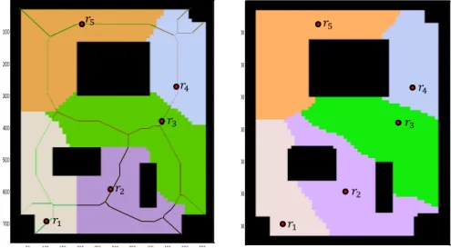
4.3 Diﬀ_{erence between geodesic and new metric Voronoi tessellation.} _{. . .} ₃₇

4.4 Equality and inequality constrains. . . 38

4.5 Discretization and graph representation. . . 39

4.6 Graph representation. . . 40

4.7 Robots motion. . . 42

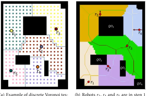
4.8 Discrete Voronoi tessellation and robots movement. . . 45

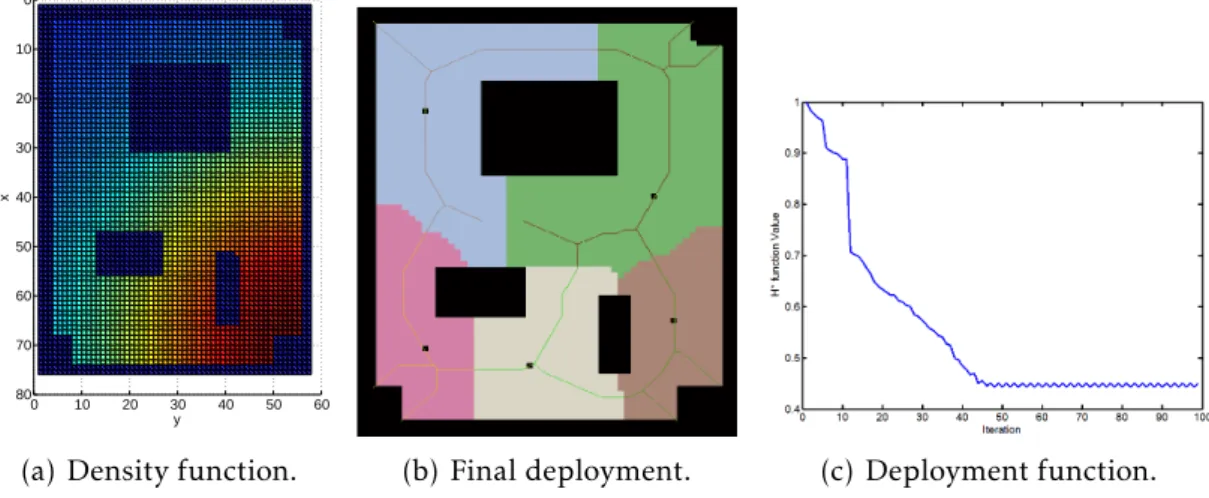
4.9 Input map and density function.. . . 47

4.10 Running the proposed algorithm for five robots. . . 47

4.11 H∗function for the first example. . . 47

4.12 Simulation with a diﬀ_{erent density function.}_{. . . .} ₄₈

4.13 Oﬃ_{ce-like map with GVD} _{. . . .} ₄₈

4.14 Density function. . . 49

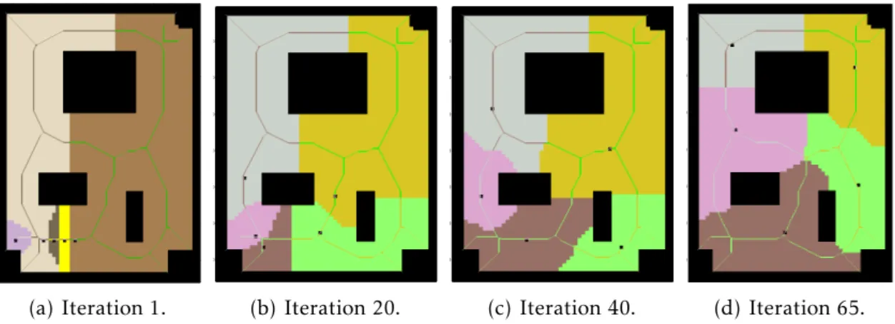
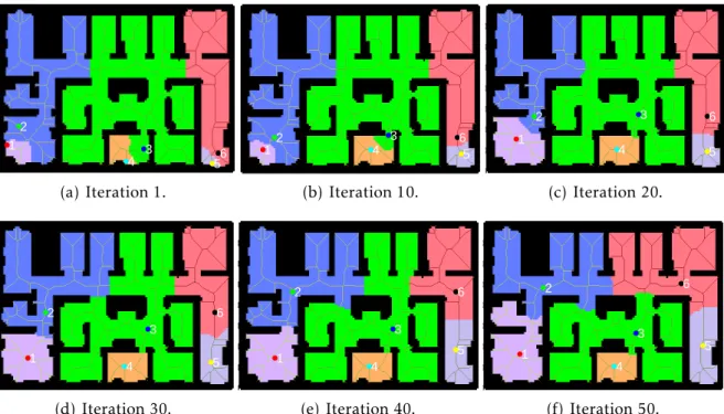
4.15 Snapshots of running the algorithm . . . 49

4.16 Result of running the algorithm on oﬃ_{ce-like map.} _{. . . .} ₅₀

(14)

5.1 Discrete approximation of the environment. . . 55

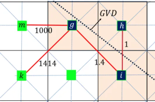
5.2 Edge modification in neighbor cell. . . 56

5.3 Assumption on obstacles. . . 57

5.4 Computing Voronoi region on a dynamic graph. . . 58

5.5 Graph neighbor nodes of cellsi. . . 59

5.6 Neighboring in the new strategy. . . 59

5.7 Projecting gradient vector. . . 62

5.8 Thread pool. . . 67

5.9 Compact adjacency list and the pattern. . . 69

5.10 Customized compact adjacency list. . . 70

5.11 Mask array. . . 72

5.12 Conflict in parallel implementation. . . 74

5.13 Running parallel wavefront algorithm. . . 75

5.14 Input descretized map. . . 78

5.15 Snapshot of a simulation run. . . 80

5.16 Final trajectory and cost function. . . 81

5.17 Input map and corresponding density function. . . 81

5.18 Iterations of running the new deployment method. . . 82

5.19 Final trajectory and cost function in Oﬃ_{ce-like Map.} _{. . . .} ₈₂

5.20 E-puck robot and robot model.. . . 83

5.21 Initial location of robots in the map. . . 84

5.22 Robots motion during the experiment. . . 85

6.1 A sketched map . . . 89

6.2 Discretizated map and directions. . . 91

6.3 Corresponding graph of the map in Fig. 6.2. . . 92

6.4 Moving between nodes. . . 92

6.5 Density function represented in graph. . . 93

6.6 Voronoi subgraph. . . 98

6.7 Robot model. . . 103

6.8 Robot system in high-level. . . 106

6.9 The map of a neighborhood in New York . . . 106

6.10 The density function. . . 107

6.11 Result of partitioning the input map by the proposed method. . . 108

6.12 Simulation result. . . 108

6.13 The map used in real robot experiment. . . 110

(15)

List of Tables

3.1 Diﬀ_{erent classes of deployment approach.} _{. . . .} ₂₄

5.1 Notations. . . 54

5.2 Result of first test. . . 76

5.3 Result of second test on two graphs.. . . 77

5.4 Result of running Dijkstra algorithm on grid graph. . . 77

6.1 Set of commands and costs in the simulation. . . 107

6.2 Comparison ofHin diﬀ_{erent methods.} _{. . . 107}

6.3 Commands applied on robots in the real experiment. . . 111

(16)

(17)

List of Algorithms

1 Dijkstra algorithm. . . 8

2 Distributed algorithm of roboti . . . 41

3 Modified Dijkstra . . . 44

4 Deployment algorithm . . . 61

5 MSSP() . . . 65

6 MSSP_CUDA . . . 71

7 KERNEL1 . . . 73

8 KERNEL2 . . . 75

9 Distributed controller . . . 95

10 FunctionFind_next_best_node(). . . 97

(18)

(19)

List of Symbols

Π_i_{(GV D)} _{Projection of the point}_p_i _{onto the GVD}

η First vertex neighbor nodes of robot

∇H Gradient ofHfunction

Ω _{Representing the environment}

ω Angular velocity

∂Ω _{Boundary of the environment}

∂Vi Boundary of the Voronoi regioni

φ Distribution density function

ai Radius of disk roboti

Co The cost map between robots and all nodes in a graph

C andC Cost/weight matrix or cost function in a graph

C_s Cost/weight of static nodes

C_d Cost/weight of dynamic nodes

c(i,j) andcij Cost between the centers of the cellsi andj or an edge

d(i,j) Distance between two nodei andj

d∗(i,j) Minimum distance between two nodei andj

E Set of edges in a graph

E_s Set of static edges

E_d Set of dynamic edges

F_V_i Free Voronoi regioni

(20)

G Graph

GGV D_i∗ Corresponds to the set of grid cells so thatd∗(P(q),P(pi))

is less thand∗(P(q),P(pj)),∀j,i

g(q,pi,G) Geodesic distance between nodesqandpi in the graphG

gi Voronoi subgraph

h Equality constraint

H,H∗,H0 Deployment function (cost function)

I Set of robot commands that links two edges

L_i,j Bisector between two Voronoi regioni andj

M Number of source (robot)

Ma A mask array for controlling wavefront algorithm

np Number of Search Points

N and|V | Number of node in graph

N_G A set of graph neighbor nodes

N_G(pi) Graph neighbor nodes of nodepi

nid Index of the neighbor of a node

o Voronoi tessellation map

P={p₁,· · ·,p_M} Configuration ofM robots

pi Configuration of roboti (vector)

pi Nodei of graph or robot position in graph

p∗_i Centroid of a Voronoi cell

˙

p_i Velocity

p_i∗ Next best node to go for roboti PathInit_T o_GV D Path from the initial point to GVD

PathGV D_T o_GV D Path from a point on GVD to another point on GVD

PathGV D_T o_Goal Path from GVD to the goal point

QO Set of obstacle

Q_{f ree} Free configuration space

(21)

xxi

q Configuration of a point in space

q_c Center of distribution function

R={r₁,r₂,· · ·,rM} Index ofMrobots

R={r1,r2,· · ·,rk} A subset ofR(R ⊆R), in which robots are neighbors

R_i A set of neighbor robots with shared Voronoi boundariesVi

Ri_V_{GV D} Position of neighbor robots which already lye onVGV D

ri Index of roboti

s Starting vertex in a path

Uc Temporary memory for cost updating

u_i Control input

V Set of nodes in a graph

V_s Static nodes

V_d Dynamic nodes

Vi Voronoi regioni

v Linear velocity

vs Source node

VGV D Set of grid cells that contain GVD curves

V Set of vertices (nodes)

Wi Tessellation regioni

W₁ andW₂ Coeﬃ_{cient of the new metric}

¯

w A constant related to the integral element of area

x0andy0 Center of Gaussian function

Xij Binary variable for edge [ij] in MILP model

[xy] The edge between nodesxandy

y Inequality constraint

(22)

(23)

List of Abbreviations

APSP All-Pair Shortest Path

AUV Autonomous Underwater Vehicle

CUDA Compute Unified Device Architecture

CVT Centroidal Voronoi Tessellation

GPU Graphics Processing Unit

GPGPU General Purpose Graphic Processing Unit

GVD Generalized Voronoi Diagram

GGVD Geodesic Generalized Voronoi Diagram

MSSP Multi Source Shortest Path

MILP Mixed Integer Linear Programming

MW Multiplicative Weighted

SSSP Single Source Shortest Path

tid Thread ID

TSP Traveling Salesman Problem

UAV Unmanned Aerial Vehicle

VD Voronoi Diagram

VMW Visibility-aware Multiplicative Weighted

WSN Wireless Sensor Network

(24)

(25)

Chapter 1

Introduction

A set of autonomous sensors, which is a networked system that can communicate

and use sensing data gathered mutually by each spatially distributed sensor node, is

known as a Wireless Sensor Network (WSN) (Suzuki and Kawabata,2008). Moreover,

according to (Bullo et al.,2009), a system composed of a group of robots that sense

their own positions, exchange messages following a communication topology, process

information, and control their motion is called a robotic network. One can find several

applications for this type of system such as surveillance, sensing coverage,

environ-ment monitoring, search and rescue, etc. In a multi-robot system, agents might

co-operate to accomplish a single task much more eﬃ_{ciently than a single-robot system.}

Also, in the case of a complex task, usually a group of robots can reach the result much

faster. Furthermore, when robots are able to sense the environment independently,

after fusing the captured data the eﬀ_{ect of a failure in some data from any}

individ-ual will not have a big impact due to the probability of having redundant information

provided by other agents.

There are two common types of strategies to coordinate a group of robots. First,

when a leading robot or central computer collects the state information of all the other

robots, the tasks and the environment to determine the appropriate motion of each

individual robot, this is called centralized strategy. In this case, the diﬃ_{culty is in}

adapting to the dynamic environment and to accommodate a large number of robots.

The second strategy is called distributed or decentralized in which each robot can

com-pute its own decision according to its states, its local environment and its interactions

with nearby robots and other entities. One benefit of this distributed system is the

possibility of reduction of the complexity of the involved algorithms such as in the

(26)

1.1indicates the communication of robots in both strategies.

(a) A centralized robotic system. All robots are contacting the server robot.

(b) A decentralized robotic system. Robots are contacting some neighbor robots in the network.

Figure 1.1: Comparison of centralized and decentralized system.

In some applications of robotic networks, an important question to be answered is:

where should each robot be placed in the environment? In the present work we show

distributed solutions to this problem which is referred as the deployment problem

byBullo et al.(2009).

In this topic, the solution is distributed in the sense that each agent depends only on

information from a small set of other agents, called neighbors, to compute its actions.

Besides, this set of neighbors is dynamic since it might change as the system evolves.

As pointed byCortes et al.(2004), this allows for scalability and robustness.

1.1 Motivation and Contributions

Due to the vast number of applications of multi-robot systems and particularly

the usage of autonomous deployment strategies, in this thesis we investigate diﬀ_erent

aspects of this research topic.

We are interested in finding optimal deployment configurations for a group of

robots. A configuration can be considered as optimal if it is a minimizer of a

func-tional encoding the quality of the deployment. The quality of deployment is usually

related to the time of response of the network after an event that needs servicing

(27)

1.1 Motivation and Contributions 3

event and the agent capabilities (speed, sensor field of view, etc). In order to minimize

the distance between agents and events, our approach applies the idea of partitioning

the environment into subregions which are then assigned to specific agents. Therefore,

each agent is responsible for attending the events in its corresponding subregion.

Figure 1.2: In this example three firefighter cars must be located over the map in such a way that in case of fire in their dedicated region, they respond in minimum time.

An example in Fig. 1.2 considers an application of determining the best station

for rescue cars in a city such that they reach the intended area in minimum time. In

locational problems, we usually have the objective of finding the best positions to place

entities such as: cars, robots or any kind of facility. Given the importance of

multi-robot deployment problem and also the fact that it is a new research topic, several

researchers are currently interested in developing new eﬃ_{cient strategies which are}

amenable to real world implementation. In this thesis we tried to address shortages

found in previous methods and also extend some works in the literature.

Contribution

In this work, our contributions are divided into 3 main parts which are listed below:

• First, we extend the previous works on multi-robot deployment by considering

safety in robots motion. In the new technique GVD is employed as a roadmap,

so that robots are forced to keep moving over the GVD. To apply this constraint

in robots path planning, we develop a new metric, which computes the shortest

(28)

the robots during deployment. Moreover, in order to compute next actions of the

robots, we developed a new eﬃ_{cient algorithm. Simulation results validates the}

applicability of the proposed method.

• A new method for deploying a team of robots by considering a continuous

move-ment of robots in a discrete representation of the environmove-ment is proposed. This

work defines a new strategy to choose the next action, such that the cost

func-tion never increases. It makes possible to address the problem of convergence

of previously proposed methods such as (Bhattacharya et al., 2013c). We also

propose a new eﬃ_{cient parallel implementation of our algorithms. In particular,}

CUDA based discrete implementation is applied to speed up the graph search

algorithm. Simulation and real robot experiments testify the performance of this

extension in Chapter5.

• While the cited deployment techniques focused on environments with two or

three dimensions represented by geometric maps, we derived a discrete setup for

deployment on a one-dimensional topological map. The topological map

repre-sents the robot’s workspace as a graph, in our case a direct graph. The idea of

this topological map on how to move a single robot in this space is developed

by Araujo et al. (2015), where a robot uses human-like commands to move in

structured environments. In fact, humans do not need to have a precise

met-ric localization to reach a destination. A simple sequence of directions such as

"turn right", "turn left", and "go straight" may be enough for a person to reach its

destination in an urban environments or oﬃ_{ce building. This methodology uses}

graph search strategies to generate such sequences of commands and deploy the

robot team in the environment. The main advantage of topological

representa-tion is to eliminate the need for precise localizarepresenta-tion of the robots. According to

these advantages, our new multi-robot deployment setup upon this framework

can be considered as a milestone in the literature of deployment. In such a way,

we do not need a specific metric for the computation (as for the humans, metric

localization is also not necessary). Given a robot that is able to move without the

(29)

1.2 Document Organization 5

motion and fast response can be achievable. Arguably, this method is suitable

for emergency responses like chasing an evader or responding to accidents. It is

important to remark that this topological based framework does not need a

com-plete and precise map as input. Thus our method will work in scenarios in which

the input map is partially known or just an image (without metric information)

is available.

Our simulation results compare our proposed method with the global solution

obtained by solving thep-median problem on the same input map. We also

exe-cuted the algorithm on a team of real robots.

1.2 Document Organization

The document is organized as follows: in the next chapter, we explain some

defi-nitions and tools that will be used in the rest of the document; In Chapter3, a review

of related papers in continuous and discrete deployment is presented; The proposed

decentralized multi-robot safe deployment is discussed in Chapter 4. In Chapter 5,

our proposed deployment algorithm with convergence proof and new implementation

will be presented;

Chapter6is dedicated to deploying robots in topological maps. This chapter also

contains: discrete topological map representation, optimal deployment in this

repre-sentation, the proof of convergence and implementation results; Chapter 7concludes

this text with a summary, list of limitations, and future directions to be pursued. We

also show the list of publications derived during the development of this work in this

(30)

(31)

Chapter 2

Background

In this chapter we present some of the tools that will be useful in the techniques

proposed in this work.

2.1 Graph (Dijkstra Algorithm)

Searchingin a graph to find a path between two locations is one of the useful

oper-ations in a routing problem. In this section, we define the Single Source Shortest Path

(SSSP) problem and review the Dijkstra algorithm (Dijkstra,1959) as its solution.

LetG={V,E,C}be a weighted graph, whereV is the set of nodes/vertices,Eis the set

of edges and finallyC is the set of non-negative weights of edges between nodes. The

SSSP problem is the one of finding the path between a source vertexsand a destination

vertextwhich has minimum total weight. An eﬃ_{cient algorithm to solve this problem}

is the so-called Dijkstra algorithm. This algorithm receives the graphGand the source

vertex s as inputs and returns the distance map, d, and array pre which contains the

pointers to the "next-hop" nodes in the shortest routes to the source (s). Algorithm 1

shows the original Dijkstra algorithm.

In this algorithm, vertices are classified into two main categories: visited nodes and

unvisited nodes. Thus, in each iteration, the closest node (q) from the unvisited nodes,

in the priority queue (Q), is removed and added to the visited part. In this way, q’s

neighbors are investigated to see whether the new path from q is closer to them or

not. Such that in lines 13 and 14 the distance map d and array pre will be updated

to the new values (this is also called “relaxation”). The evolution of this process is

(32)

Algorithm 1:Dijkstra algorithm.

Input: G, s

Output: d, pre

1 d(s)←0// Distance from source to source 2 foreachv∈V do// Initialization of distance 3 ifv,sthen

4 d(v)← ∞

5 pre(v)←undef ined // Previous node in optimal path from source

6 Q←v // Add allvin the listQ

7 while(Q ,∅)do

8 q←arg min q′_∈Q d(q

′₎_{// return vertex in}_Q_{with minimum distance to source}

9 Q←Q\q// RemoveqfromQ

10 foreachw∈ N_G(q)do // For each graph neighbor node ofq 11 d′←d(w) +C(w,q)

12 ifd′ < d(q)then// Relaxation

13 d(q)←d′ // Update the cost of neighbor nodes ofq 14 pre(q)←w// by considering new cost from source toq

of a naive implementation is O(|V |2_{), where}_{|V |} _{is the number of nodes, but other}

im-plementations using a fibonachi heap(Cormen et al.,2001), have a much better result

O(|E|+|V |log|V |), where|E|is the number of edges.

2.2 Generalized Voronoi Diagram (GVD)

Consider the set of obstaclesQO={QO₁,· · ·,QO_n}defined in a planar configuration space. This set induces a structure called Generalized Voronoi Diagram (GVD). A set

of points in the free configuration space (Q_{f ree}) is defined as the Voronoi region (V_i) of

the obstacle QO_i, if these points are closer toQO_i than to all the other sites, where a

site is the same as an obstacle in this case (Choset et al.,2005).

Vi={q∈ Qf ree|d(q,QOi)≤d(q,QOj),∀j,i}, (2.1)

(33)

2.2 Generalized Voronoi Diagram (GVD) 9

with distinct gradient vectors:

L_i,j={q∈ Q|d(q,QO_i) =d(q,QO_j) and∇d(q,QO_i),∇d(q,QO_j),j ,i}. (2.2)

The points in L_i,j (that are part of the GVD) are those in which QO_i and QO_j are

the closest obstacles. Therefore we can define the set:

Vi,j ={q∈ Li,j| ∀h, d(q,QOi)≤d(q,QOh)}. (2.3)

This last definition allows us to formally define the GVD:

GV D=[

i

[

j

Vi,j. (2.4)

In Fig.2.1an example of definition given by Eq. (2.4) is shown.

d(q,𝒬𝒪) q

𝒬𝒪

ℒ,

𝑉,

d(q,𝒬𝒪)

𝒒a

𝒒goal

𝒒goal′

𝒒′a

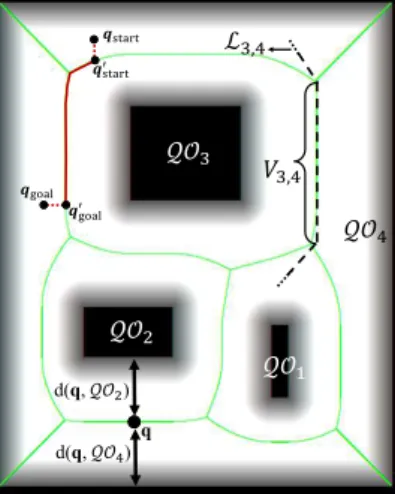
Figure 2.1: Example of GVD (green line).QO₁,QO₂,QO₃ andQO₄ are the obstacles or sites. q is an equidistant point between sitesQO₂ andQO₄ that belongs to the GVD. The lineL₃_,₄is a bisector between sitesQO₃andQO₄. V3,4is the part of lineL3,4which

is a portion of the GVD.

An interesting feature of the GVD is that it can be used as a roadmap for path

planning. This means that it is always possible to plan a path from a pointqstart∈ Qf ree

(34)

2005) (see Fig. 2.1). Given the fact that the GVD is formed by points equidistant from

the closest obstacles, in general it provides a safe route for the motion. Therefore, if

several excursions in the environment are demanded from robots and a map of this

environment is given, it is worth computing the GVD and then use it as a roadmap for

such excursions. Given a GVD, planning a path is a matter of running a simple graph

search. In the present work we use GVDs to incorporate safety in a multi-robot motion

and simplify the workspace.

2.3 Voronoi Tessellation

In this section, to explain Voronoi tessellation we use the same definitions in the

context of GVD (Section2.2). In the free configuration space (Q_{f ree}) of an environment,

Voronoi tessellation is defined as regions associated to a set of points. If we consider

to P ={p₁, . . . ,p_M}be the sites or points distributed over Q_{f ree}, instead of obstacles in GVD, where pi ∈ Qf ree indicates the position of point i, the setV ={V1,· · ·,VM}is the

corresponding Voronoi tessellation given by:

Vi={q∈ Qf ree|d(q,pi)≤d(q,pj),∀j ,i}, (2.5)

where, d is the distance function, so that if we considerd as Euclidean distance it can

be written: d(q,p_i) =||q−p_i||. Moreover, the boundary between two Voronoi regionsVi

andVj is:

L_ij ={q∈ Q_{f ree}|d(q,pi) =d(q,pj), j ,i}. (2.6)

If we denote the boundary of a Voronoi regionVi by∂Vi, a neighbor site ofpi can

be defined as:

R_i ={pj ∈P |∂Vi∩∂Vj ,∅, i,j}. (2.7)

An example of environment with four sites and their corresponding Voronoi cells

(35)

2.4 Locational Optimization Based Deployment 11

cells which are associated to each point pi (based on Euclidean distance). Also the

boundaries between regions are shown by lines. It should be noticed that in a Voronoi

tessellation we have: SM

i=1

Vi =Qf ree, and alsoI(Vi)TI(Vj) =∅,∀i,j, whereI(Vi) returns

the interior of Voronoi regioni.

Figure 2.2: A set of sites (pi) with corresponding Voronoi regions(Vi).

2.4 Locational Optimization Based Deployment

In this section we present the general problem of deployment considering the

loca-tional optimization framework proposed by Cortes et al.(2004), which is the basis to

our work.

2.4.1 Problem Definition

Consider a team ofM robots has to be distributed on a bounded environmentΩ _∈

R2_{. The configuration of robots is defined by} _P ₌_{p₁_{, . . . ,}_p_M_}_{, where} _p_i _∈ Ω_{. In this}

setup, robots must cover the whole environment, so that each of them is responsible to

a Voronoi cellVi, whereV ={V1,· · ·,VM}, and M

S

i=1

Vi =Ω. The quality of this deployment

(36)

H(P,V) =

M

X

i=1

H(pi,Vi), (2.8)

and,

H(p_i,Vi) =

Z

Vi

d(q,p_i)2φ(q)dq, (2.9)

whered denotes the distance function between the robots and points. Diﬀ_erent

met-rics can be used to compute the distance in an environment. For instance, in Fig 2.3

a comparison between Euclidean and geodesic distance in a non-convex environment

is shown. While Euclidean distance between pand qis shorter and suitable for con-vex environment, geodesic distance is more realistic in a non-concon-vex scenario (dashed

line), in the sense of considering obstacles.

𝓠𝓞

Figure 2.3: Euclidean and geodesic (dashed line) distance in a non-convex environ-ment.

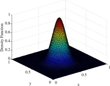
In Eq. (2.9), for each point q ∈ Ω_{, the function} _φ(_q_{) denotes the importance of}

the point. We call this functionφ :Ω _→R+_{, a distribution density function. In other}

words, φ shows the priority of servicing events in the environment by robots, hence

the regions with higher priority have higher weights. In Fig. 2.4, an example of

Gaus-sian function, as a density function, in a planar environment is shown, in which the

center of environment (corresponding to the center of function) needs more priority to

be covered by robots. Throughout our text we assume that robots have access to the

in-formation of density function before starting the deployment process. However, when

the robots do not know this function, it can be learned online by techniques developed

in (Schwager et al.,2009) based on sensor data.

(37)

deploy-2.4 Locational Optimization Based Deployment 13

0

0.5

1

0 0.5

1 0 0.2 0.4 0.6 0.8 1

x y

Density Function

Figure 2.4: Example of density function in a 2D environment. The center of Gaussian function is placed at the pointqc = [0.5,0.5]T and its support (spread of the blob inx

andy) is equal tokq−q_ck<0.3.

ment, a team of robots cover an area to optimize the cost function (H), which directly

depends on the distance between robots and points. Therefore, the better is the

dis-tribution of robots over the environment, the lower is the value ofH. In this way, our

deployment problem is translated to a minimization problem.

According to the work byCortes et al.(2004), if we consider a convex environment

with Euclidean distance function d, it is easy to show that if robots are located on

centroidof Voronoi partitions, the minimum value ofHfunction will be obtained. The

centroid can be defined by:

p∗_i =

R

Viqφ(q)dq

R

Viφ(q)dq

. (2.10)

Therefore, to minimize the function in Eq. (2.8), robots must be driven to the

cen-troid of their Voronoi tessellation. In such a way, the result partitions are known as

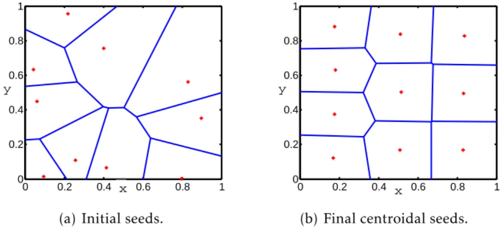
Centroidal Voronoi Tessellation (CVT). Lloyd’s algorithm is a well-known iterative and

discrete approach for CVT which is proposed byLloyd(1982). By having an

environ-ment with some points as sites, in each iteration of this algorithm the Voronoi

(38)

0 0.2 0.4 0.6 0.8 1 0

0.2 0.4 0.6 0.8 1

y

x

(a) Initial seeds.

0 0.2 0.4 0.6 0.8 1

y

x

(b) Final centroidal seeds.

Figure 2.5: Example of CVT with 10 points as sites or seeds.

This process will stop when the current sites (points) corresponding to the centroids

of the next iteration. An example of this method is shown in Fig. 2.5. In this thesis,

the most part of our works is based on the continuous version of this algorithm which

is proposed by Cortes et al. (2004). In their work, the kinematic model of a robot is

defined as:

˙

pi=ui, (2.11)

whereui is the robot control input. Also in a continuous setup, the following control

law guarantees that the system converges to a CVT:

ui=−k(pi−p∗i), (2.12)

where k is a positive weight. According to Eqs. (2.8) and (2.9), finally, the

gradient-descent control law that leads the robots to CVT, in Euclidean distance (d) andf(x) =

x2, can be computed as (Cortes et al.,2004):

∂H

∂pi

= 2

Z

Vi

φ(q)(p_i−p∗_i)dq. (2.13)

It is important to notice that H is a non-convex function, which implies that the

(39)

2.4 Locational Optimization Based Deployment 15

2.4.2 p

-Median Problem

The locational optimization problem in Section2.4.1was defined in a continuous

setup, but if we discretize the input map into cells and represent it as a graph, then the

deployment problem can be considered as ap-median problem. Inp-median problem

the main objective is to find location ofpfacilities (or medians) relative to a set of users

or customers, in which the sum of the shortest demanded distance from customers

to facilities is minimized. The p-median problem was initially proposed by Hakimi

(1964). This problem is classified as NP-hard, therefore many heuristic and

meta-heuristic methods have been proposed to solve it (Mladenovic et al., 2007; Rolland

et al.,1996). The mathematical model of this problem can be defined as follows.

Consider a set of possible locations for facilitiesS={1,. . . ,M}, and a set of customers

Y ={1,. . . ,N}. d is a distance function, in whichd(i,j) indicates the shortest distance

from customer i to facility j (i ∈ Y and j ∈ J, where J is a subset of S). Thus, the

objective is to minimize the given function:

F= X

i∈Y

min

j∈J d(i,j), (2.14)

whereJ ⊆S and|J|=p. An example of this problem with 7 customers and 2 facilities

is shown in Fig. 2.6.

𝑝

Figure 2.6: A solution ofp-median problem with 2 facilities and 7 customers.

According to the above explanation, in this thesis, to validate the eﬃ_{ciency of our}

(40)

the optimum result achieved by solving its corresponding p-median problem. Such

that, in p-median problem, N points (vertices or customers) are assigned toM robots

(facilities).

2.5 GPU (Graphics Processing Unit) and Compute

Uni-fied Device Architecture (CUDA)

GPGPU (General Purpose Computing on Graphics Processing Unit) has become a

hot topic nowadays in several fields that demand high performance hardware. This is

a method of using the GPU (Graphics Processing Unit) to perform computations for

tasks other than graphics, such as astrophysical modeling, signal/image processing,

electromagnetic field computation, etc. The great advantage of this strategy is the

parallel nature of graphics processing.

Compute Unified Device Architecture (CUDA) was developed by NVIDIA as a

par-allel computing solution which covers both parpar-allel software and hardware

architec-ture. It can execute thousands of threads at the same time, thus CPU sees a CUDA

device as a multi-core co-processor.

2.5.1 Software Model:

The execution in CUDA is based on threads. Hence programmers must define

the number of threads for their usage. A group of threads creates a block. Inside a

block, threads can cooperate together by eﬃ_{ciently sharing data through some fast}

shared memory and synchronizing their execution to coordinate memory accesses.

Each thread is identified by itsthread ID, which is the thread number within the block.

A block can be defined as a 2 or 3 dimension array to simplify complex addressing.

For example, in the case of 2-D block with size (Sx,Sy), the thread ID of a thread with

index (x,y) isx+y∗Sx.

The maximum number of threads within a block is limited, but blocks with the

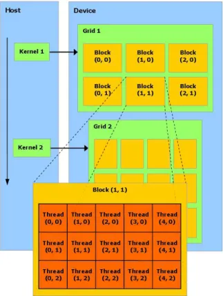
same size and dimension can be joined into a grid (See Fig. 2.7). A grid can be

(41)

2.5 GPU and CUDA 17

Figure 2.7: Threads in memory (NVIDIA,2007).

launched at the same time is very large. However, it must be noticed that threads in

diﬀ_{erent thread blocks from the same grid cannot communicate and synchronize with}

each other.

As illustrated in Fig. 2.8, the software architecture is composed of several layers.

Developers use the CUDA API (Application Programming Interface) in their

applica-tions and also CUDA runtime and CUDA driver to run and launch their application

on GPU.

CUDA as a programming interface provides the ability to contact and use GPU for

users familiar with programming language. In fact, CUDA runtime library contains

functions to control and accesshost(GPU) andguest(CPU) space.

Kernels

An important step in CUDA programming is defining a C function, which is called

(42)

Figure 2.8: Compute Unified Device Architecture Software Stack (NVIDIA,2007).

N times in parallel byN diﬀ_{erent CUDA threads. The user can define a kernel by}

writ-ing the keyword __global__ at the beginnwrit-ing of the function declaration. Furthermore,

when calling it, the number of blocks and threads, which will be used in the GPU, is

set between " < < <· · ·> > > " after the name of the function. A simple program for

adding two vectors is defined in the code below (Sanders and Kandrot,2010). In the

first code, the function for summing two vectors in CPU and storing the result into

vector C is shown. Inside the code, a loop is applied to repeat the sum operator N

times, whereN is the size of the input vectors.

1 void _VecAdd₍ int _*_a_, int _*_b_, int _*_c ₎

2 {

3 for ₍_i_=0; _i _< _N_; _i₊₊₎

4 {

5 c[i] = a[i] + b[i];

6 }

7 }

In the case of CUDA, the same function, for adding two vectors, will be defined as

the following code (Sanders and Kandrot,2010):

1 void _VecAdd₍ int _*_a_, int _*_b_, int _*_c ₎

2 {

(43)

2.5 GPU and CUDA 19

4 if ₍_tid _< _N₎

5 c[tid] = a[tid] + b[tid];

6 }

Diﬀ_{erently from the function which was defined in CPU, here there is no loop.}

This means the line inside the function runs N times in N threads in a parallel way.

Each thread that executes the kernel is given a unique thread ID that is accessible

within the kernel through the built-inthreadIdx variable. The Code below shows how

the number of threads and other input parameters are passed (Sanders and Kandrot,

2010):

1 # include _{<iostream >}

2 # define _{N 10}

3 int _main₍ void ₎

4 {

5 int _a_[_N_], _b_[_N_], _c_[_N_]; // Input array from CPU

6 int _*dev_a_{, *}dev_b_{, *}dev_c; // variables for GPU

7 Initit(a,b,c);// Initialize a,b and c

8 // allocate the memory on the GPU

9 cudaMalloc( (void_**)&_{dev_a}_, _N _* sizeof₍int_{) ) ;}

10 cudaMalloc( (void_**)&_{dev_b}_, _N _* sizeof₍int_{) ) ;}

11 cudaMalloc( (void_**)&_{dev_c}_, _N _* sizeof₍int_{) ) ;}

12 // fill the arrays ’a’ and ’b’ on the CPU

13 cudaMemcpy( dev_a, a, N_* sizeof₍int_), _{cudaMemcpyHostToDevice}_);

14 cudaMemcpy( dev_b, b, N_* sizeof₍int_), _{cudaMemcpyHostToDevice}_);

15 VecAdd<<<1,N>>>(dev_a, dev_b, dev_c);

16 cudaMemcpy( c, dev_c, N_* sizeof(int), cudaMemcpyDeviceToHost );

17 for (int i=0; i<N; i++)

18 printf("\%d+\%d=\%d \n",a[i],b[i],c[i]);

19 cudaFree(dev_a);

20 cudaFree(dev_b);

21 cudaFree(dev_c);

22 return _0;

23 }

The number of threads is directly related to the problem which is defined by the

(44)

block is equal to the size of the input vector or N = 10. On current GPUs, a thread

block may contain up to 1024 threads.

It can be seen in the code that before using the variables in GPU they should be

allocated bycudaMalloc(). This function behaves very similarly to the standard C call

malloc(), but it tells the CUDA runtime to allocate the memory in the device.

An-other useful function is cudaMemcpy, similarly to the standard C function memcpy.

This function copies data from host to guest and the other way around (Sanders and

Kandrot,2010).

(45)

2.5 GPU and CUDA 21

2.5.2 Hardware Model:

CUDA has two main taxonomies: the GPU is called thedeviceand the CPU is called

thehost. It also consists of a set of multiprocessors (See Fig. 2.9). Each multiprocessor

has access to the four following memory types (NVIDIA,2011):

• shared memory, which is common to all thenprocessors,

• A set of 32-bit registers per processor,

• A read-onlyConstant cache that is shared between all processors,

• A read-onlyT exture cachethat is also shared by all processors.

The two last types of cache memory speed up reading from constant and texture

memory space. The device memory is accessible from all multiprocessors, hence they

can communicate to each other via this memory.

Atomic operators:

In multi-threading applications, a common problem which must be avoided is race

condition. It happens when two or more threads want to operate on the same shared

memory concurrently. Atomic operations are often used to prevent race conditions. An

atomic operation is capable of reading, modifying, and writing a value back to memory

without the interference of any other threads, which guarantees that a race condition

would not occur. Atomic operations in CUDA generally work for both shared memory

and global memory. For example:

int atomicAdd(int_* address, int val);

ThisatomicAddfunction can be called within a kernel. When a thread executes this

operation, a memory address is read, has the value of "val" added to it, and the result

is written back to memory. There are other operators for the main mathematical and

(46)

2.5.3 New CUDA Hardware Model

Because of the complexity of managing these diﬀ_{erent kinds of memories, NVIDIA}

proposed a new version of CUDA (NVIDIA, 2014). In CUDA 6, they introduced

unif orm memory to have a shared data between CPU and GPU. Therefore, this

mem-ory can be accessed by using a single pointer. Fig. 2.10illustrates this new architecture.

Figure 2.10: New architecture in CUDA 6,NVIDIA(2014).

In Chapter5, we are going to show a version of the proposed distributed algorithm

(47)

Chapter 3

Related Work

3.1 Multi-Robot Deployment

Multi-robot deployment problems have attracted attention of several groups due

to the great applicability of robotic networks. A major category in multi-robot

de-ployment control schemes is the one based on artificial potential fields or force fields:

Parker (2002) developed a distributed algorithm to coordinate a group of robots to

monitor multiple moving targets. This strategy was based on the use of attractive and

repulsive force fields. Reif and Wang (1999) proposed artificial force laws between

pairs of robots or robot groups to control Very Large Scale Robotic (VLSR) systems.

Since the force laws may reflect the "social relations" among robots, this method was

namedSocial Potential Field. Similarly,Howard et al.(2002) presented a potential field

based method in which the final force for each robot is achieved by summing both

the repulsive forces from obstacles and the repulsive forces from other robots. The

objective in this case is to maximize the environment coverage. Poduri and Sukhatme

(2004);Popa et al.(2004);Ji and Egerstedt(2007) also used potential field based

con-trollers for coverage, formation control and preservation the connectivity of agents in

an ad hoc network.

Another important category is the one built upon theLocational Optimization

Frame-work (Okabe et al., 1992). This was initially proposed by Cortes et al. (2004). The

authors in (Cortes et al., 2004) present a distributed and asynchronous approach for

optimally deploying a uniform robotic network in a domain based on a framework for

optimized quantization derived byLloyd(1982). Each agent (robot) follows a control

law, which is a gradient descent algorithm that minimizes the functional encoding the

(48)

infor-Table 3.1: Diﬀ_{erent classes of deployment approach.}

Methodology NC1 NE2 Con3 Het4 GB5 CP6 Dec7

Cortes et al.(2004) - - X _- _- X X

Pimenta et al.(2008) X X X X _- X X

Schwager et al.(2009) - - X _- _- X X

Breitenmoser(2010) X X X _- _- X X

Stergiopoulos and Tzes(2011) - - X X _- _- X

Schwager et al.(2011) X _- X _- _- X X

Mahboubi and Sharifi(2012) - - X _- _- _- X

Durham and Carli(2012) X X _- X X X X

Yun and Rus(2013) X X _- _- X X X

Bhattacharya et al.(2013b) X X X _- X X X

Sharifi et al.(2014) - - X _- _- X X

Sharifi et al. (2015), Pierson et al.

(2015) - - X X - X X

1 _{NC: Non-Convex} 2 _{NE: non-Euclidean} 3 _{Con: Continuous}

4 _{Het: Heterogeneous} 5 _{GB: Grid-Based} 6 _{CP: Convergence-Proof} 7_{Dec: Decentralized}

mation about the position of the robot and of its immediate neighbors. Neighbors are

defined to be those robots that are located in neighboring Voronoi cells. Besides, these

control laws are computed without the requirement of global synchronization. As we

explained in Section 2.4, the functional also use adistribution density function which

weighs points or areas in the environment that are more important than others. Thus,

it is possible to specify areas where a higher density of agents is required. This is

im-portant if events happen in the environment with diﬀ_{erent probabilities in di}ﬀ_erent

points. Furthermore, this technique is adaptive due to its ability to address changing

environments, tasks, and network topology.

Coverage in the sense of (Cortes et al., 2004) is illustrated in Fig.3.1. In this

fig-ure four robots are deployed in a convex environment. The density function used is

uniform, so all points of the environment have identical priority. At the beginning,

the environment is divided in four Voronoi regions, one for each robot. The technique

proposed inCortes et al. (2004) generates velocity vectors for each robot so that they

continuously move towards the centroids of their respective Voronoi regions, which, as

(49)

3.1 Multi-Robot Deployment 25

be proved that the multi-robot system converges to a configuration where the

environ-ment is equally distributed among the robots or, in the case of non-uniform density

functions, is distributed according to this function. It is important to notice that, even

in convex workspaces, real world implementations of this methodology require global

and precise metric localization for the robots and non-linear control strategies to

fol-low the velocity vectors.

(a) Time 1. (b) Time 4. (c) Final.

Figure 3.1: Deployment of 4 robots in a convex environment using the approach pro-posed by Cortes et al. (2004). In (a) and (b) the “*" sign indicates the center of the Voronoi regions, which represent the current goal position for each robot. Voronoi regions are highlighted with diﬀ_{erent colors.}

Diﬀ_{erent extensions of the framework devised by} _{Cortes et al.} ₍₂₀₀₄_{) have been}

proposed in the literature. Table 3.1 lists some of the articles with their properties:

convex or non-convex, Euclidean or non-Euclidean, continuous or discrete,

hetero-geneous or homohetero-geneous teams, grid-based or geometric, with convergence-proof or

without, and decentralized or centralized. In this work we focus on two main schemes:

continuous anddiscrete. Hence, in the following we are going to review the literature

of both schemes separately.

3.1.1 Multi-Robot Deployment in Continuous Space

After the initial work by Cortes et al. (2004), which can only be applied to

con-vex and static environments, Pimenta et al. (2008) applied geodesic distance for

de-ploying a team of heterogeneous robots in non-convex environments. The problem

(50)

et al. (2010) to solve a task of simultaneous coverage and intruders tracking. For a

similar problem, Schwager et al. (2009) developed an adaptive controller, such that

robots learn the distribution of sensory information (density function) during the

de-ployment. Another approach for deploying multiple robot in non-convex environment

was presented byBreitenmoser (2010). In order to avoid collision with obstacles, the

authors combined the deployment control law with a local planner (Tangent Bug).

Most of the previously cited works can be classified as Voronoi-based coverage

strategies since they use the centroid of the current Voronoi region in their controller.

However, there are other papers that provide alternative partitioning techniques.

Ster-giopoulos and Tzes(2011) propose a method for area-coverage in the case where the

sensors are heterogeneously range-varied. In this method, diﬀ_{erently from what we}

call CVT (Centroidal Voronoi Tessellation (Cortes et al.,2004)), as a standard method

for tessellation, they performed a diﬀ_{erent space-partitioning scheme, which was}

pro-posed previously by Tzes and Stergiopoulos (2010). In this work, they developed a

coverage-oriented modified Voronoi, based on diﬀ_{erent sensing areas from the set of}

heterogeneous nodes (agents) and preserved the convexity of the Voronoi regions. In

their simulation result, they claim that the proposed method, in the case of

heteroge-neous networks, can increase the total sensed area in the same time as the standard

tessellation method.

Multi-robot deployment with the use of multiplicative weighted Voronoi

(MW-Voronoi) diagram in an obstacle free environment is discussed byMahboubi and

Shar-ifi (2012). In this work, the authors consider diﬀ_{erent weights for each robot in the}

process of constructing the Voronoi tessellation. Moreover, in the presence of

obsta-cles, the tessellation is done by applying a visibility-aware multiplicatively weighted

Voronoi (VMW-Voronoi) diagram. Therefore, it is possible to have an uncovered

re-gion, where it is not only invisible from the robots viewpoint, but also will not be

considered in the Voronoi tessellation.

A deployment strategy for multi-agent system that considered communication

de-lay and sensors eﬀ_{ectiveness variation is presented by}_{Sharifi et al.}₍₂₀₁₄_{). In this work}

(51)

be-3.1 Multi-Robot Deployment 27

havior, which is called Guaranteed Multiplicative Weighted (GMW) Voronoi. Agents

with diﬀ_{erent types of dynamics are taken into account by the same authors in (}_Sharifi

et al.,2015). They used MV-Voronoi partitioning approach to find the corresponding

region for each robot based on their dynamics.

Caicedo-Nunez and Zefran (2008a) and Caicedo-Nunez and Zefran (2008b)

con-sidered non-convex environments by constructing a diﬀ_{eomorphism to convex regions}

with isolated obstacles in its interior, in which regular Voronoi coverage can be applied.

As they mentioned besides significant computational challenges, the generated

solu-tion may diﬀ_{er from the corresponding optimal coverage solution in the original space.}

They addressed these shortages in the work byCaicedo-Nunez and Zefran(2008a) by

characterizing a set of stationary points for the Lloydś_{algorithm in general regions.}

The DisCoverage1 algorithm in a convex environment for multi-robot exploration,

based on the work ofCortes et al.(2004), is proposed byHaumann et al.(2010).

More-over, an extension of this algorithm for non-convex environments in the specific

con-text of exploration, by including the idea of using geodesic distance as the work of

Pimenta et al.(2008), is done byHaumann et al.(2011). This method transforms

non-convex environments into star-shaped domains and use these new domains to apply

the DisCoverage algorithm.

Ny and Pappas(2013) consider three related classes of problems: coverage control,

spatial partitioning, and dynamic vehicle routing. They proposed an adaptive

algo-rithm which was based on stochastic gradient algoalgo-rithms that optimize utility

func-tions in the absence of a priori knowledge of event location distribution.

The present work further extends the works by Pimenta et al. (2008) and

Bhat-tacharya et al.(2013c). In the first part of our work, we incorporate safety as a

param-eter into the deployment problem. By merging diﬀ_{erent Voronoi diagrams,}

includ-ing the well known Generalized Voronoi Diagram (GVD) (Choset et al.,2005) and by

considering a constrained optimization problem in the context of the Locational

Op-timization Framework, we generate safe routes for the robots during deployment and

also after deployment when servicing a given point of the environment. We propose

1_{In (}_{Haumann et al.}_,₂₀₁₀_{), using Voronoi partition-based coverage algorithm in multi-robot}

(52)

a new Voronoi Diagram which is built according to a new metric that takes into

ac-count shortest paths that traverse the GVD. Moreover, in order to consider real world

environments, we devise a new eﬃ_{cient algorithm to compute the next actions of the}

robots in the same spirit of the one proposed byBhattacharya et al.(2013c).

In the second part, we will develop a new algorithm to address the problem of

convergence of previously proposed methods such as (Bhattacharya et al.,2013c) and

(Bhattacharya et al.,2013b). This work defines a new strategy to choose the next action,

such that the cost function never increases.

We also contribute in the proposition of new eﬃ_{cient implementation methods of}

our algorithms. We propose a GPU (Graphics Processing Unit) based implementation.

3.1.2 Multi-Robot Deployment in Discrete Space

While our contributions are mostly based on the continuous setup ofPimenta et al.

(2008) and Bhattacharya et al.(2013c), in the implementation part we applied a

dis-crete scheme, graph representation, to present the map and robots motion. Thus we

will briefly survey some of the discrete techniques in the literature of multi-robot

de-ployment. For a chronological order and characteristic of each method presented,

please refer to Table3.1.

Yun and Rus(2013) describes a decentralized algorithm for locational optimization

on graphs. The technique creates an undirected graph from the map and computes

a Voronoi tessellation on the graph. Finally, based on the optimization framework,

robots move to the desired nodes.

Some works also inspired by the locational optimization framework considered the

discretization of the environment by grid cells to facilitate computation in complex

environments. Durham and Carli(2012) considers a discrete partitioning and

cover-age optimization algorithm for robots with short-range communication. In this case

a discrete setup was presented, in which a discrete deployment functional is defined.

The authors proved that their algorithm converges to a subset of the set of centroidal

(53)

parti-3.2 GPU Based Graph Search and CVT 29

tion. Gossip communication2 was used to allow information exchange among the

agents. In the work by Bhattacharya et al. (2013c), the environment was also

dis-cretized to allow the numerical computation of the environment partition (geodesic

Voronoi diagram), but in that case the context was the one of generating an

approxi-mation to the continuous setup. In the same spirit of approximating the continuous

setup,Bhattacharya et al.(2013b) discretized the environment and used a graph-based

approach inspired by Dijkstra algorithm (Dijkstra,1959) to directly compute the

pro-posed control law in an eﬃ_{cient manner in general Riemannian manifolds with}

bound-aries.

Among all previous approaches surveyed, the most similar to the one presented in

this work is Yun and Rus(2013). The authors computed the Voronoi partitions upon

an undirected graph that topologically encodes the environment. However, the

au-thors still use the original 2D metric map to control the robots, what, similarly to all

other previous strategies, makes the method dependent on precise localization. The

approach proposed in the present work improves on that point since all steps of the

method execute on the topological map. This highly simplifies the actual robot

imple-mentation, as will be shown in Chapter6.

3.2 GPU Based Graph Search and CVT

Graph is one of the most useful approaches in representing topology of a system in

diﬀ_{erent fields. Finding the shortest path between nodes in a graph is a fundamental}

problem. The problem is called Single Source Shortest Path (SSSP) when the distance

between one node (vertex) to all the other nodes is considered in a weighted graph.

The most popular sequential algorithm for solving this problem is Dijkstra (Dijkstra,

1959) which can run on non-negative edge weight graphs. The simplest version of the

Dijkstra algorithm uses an array structure to maintain the graph, thus the complexity

of it isO(|V |2_{), where}_{|V |}_{indicates the number of nodes in the graph. Di}ﬀ_{erent versions}

of the data structure have been proposed in order to speed up the algorithm. By using

2_{A short-range communication with asynchronous and unreliable communication between nearby}

(54)

Fibonacci heap (Cormen et al.,2001) its running time is bounded byO(|V |log|V |+|E|),

where|E|is the number of edges. Meyer and Sanders(2013) introduced ∆_Step _which

ordered nodes by using bucket representation with size ∆_{, and each bucket may be}

processed in parallel. They also did a review in detail of another formulation of

par-allel SSSP. Madduri et al.(2007) do an eﬃ_{cient implementation of this algorithm for}

multi-thread parallel computer (Cray MTA-2). By improving hardware for parallel

processing, General Purpose Graphical Processing Unit (GPGPU) has become a

pop-ular topic being a solution not only in Graphics, but also in diﬀ_{erent applications in}

diﬀ_{erent areas. It has high power of parallel processing with lots of threads and low}

price. Moreover, it was introduced a SDK, which makes programming easy for

devel-opers. CUDA was one of the most famous parallel purpose hardware (graphic card)

in-troduced by NVIDIA (we explained the architecture in Section2.5). Some researchers

have been working on SSSP in order to implement it on CUDA.Harish and Narayanan

(2007) used compact adjacency list to represent the graph and presented a fast

imple-mentation of graph search algorithms such as breadth-first search, SSSP and All-Pairs

Shortest Path (APSP) in CUDA.Martin et al.(2009) proposed several solutions for SSSP

based on Dijkstra. They compared Dijkstra algorithm implemented on CUDA with

ad-jacency list and CPU, based on Fibonacci structure on diﬀ_{erent random graphs. Also,}

they claim that their algorithm overcomes the problem in (Harish and Narayanan,

2007) for not using the atomic function.

APSP (All Pairs Shortest Path) is another challenge in graph search, in which paths

between all pairs must be found. In general, parallel algorithms for solving this

prob-lem can be classified in two categories: methods that run SSSP iteratively and methods

based on Floyd-Warshall algorithm (Floyd,1962). An example of the first category is

the work ofHarish and Narayanan(2007). Usually, this type of approach requires

re-dundant computation and also large memory space. A good literature review of APSP

is discussed in (Katz and Kider,2008). Moreover, Katz and Kider(2008) adapted the

original Floyd-Warshall algorithm to become a hierarchically parallel method. They

run the proposed method on large graphs on a single GPU with multiple processors