Abstract—This paper presents a mixed integer linear programming model of scheduling parallel batch processing machines that minimizes total tardiness of jobs. The proposed model incorporates several practical issues such as unequal job ready times, arbitrary job sizes, and arbitrary job processing times. Due to the NP-hardness of problem under study, this paper proposes a hybrid differential evolution (HDE) algorithm to solve large-sized instances. To avoid the premature convergence, simulated annealing is incorporated in HDE to help the algorithm escape from local optima. The performance of presented model and proposed algorithm is verified by extensive experiments. The related results show the effectiveness of the proposed model and HDE for small and large-sized problems. In addition, some statistical tests are conducted to find the best performance of HDE due to its parameters.
Index Terms—Scheduling, Parallel batch processing machine, Differential evolution, Simulated annealing, Total tardiness
I. INTRODUCTION
HIS paper addresses the scheduling problem of batch processing machines. Batch processing machines (BPM) can process several jobs simultaneously. These machines are commonly used in manufacturing industries such as wafer fabrication, metal working, burn-in ovens and testing electrical circuits. In recent years, there have been many studies of the BPM scheduling problem. Mathirajan and Sivakumar [1] and Potts and Kovalyov [2] provide an extensive review on scheduling with batching.
The problem under study considers a set of BPM in parallel which commonly used to test printed circuit boards. The BPM can process a batch of jobs as long as the total size of all the jobs in the batch does not exceed the machine capacity. The processing time of the jobs, the ready time of the jobs and their size are different and are given in advance. Consequently, the processing time of the batch is equal to
Manuscript received June 17, 2012; revised August 07, 2012.
A. Jafari is the assistant professor in the Department of Industrial Engineering, University of Science and Culture, Tehran, Iran, (e-mail:
S. Hassani is with Department of Industrial Engineering, University of Science and Culture, Tehran, Iran, (e-mail: [email protected]).
P. Chiniforooshan is with the Department of Industrial Engineering, Science and Research Branch, Islamic Azad University, Tehran, Iran (corresponding author to provide phone: +989125104151, fax: +982155634107, e-mail: [email protected];
the longest processing job in the batch and a batch can be processed only when all the jobs in a batch are ready.
A mixed-integer linear programming (MILP) model is proposed to formulate the problem under study. The objective is to minimize the total tardiness in order to maximize on-time delivery performance. A special case of the problem, when the processing times of all the jobs are identical, the batch formation problem is equivalent to the bin packing problem which is known as a NP-hard problem [3]. Consequently, the under study problem is NP-hard. Therefore, meta-heuristic algorithms, such as genetic algorithm [4], simulated annealing [5, 6] are used to find a good solution for this problem.
Differential evolution (DE) is a novel evolutionary algorithm recently introduced by Storn and Price [7] for optimization problems over continuous spaces. Due to its ease of use, fast convergence and robustness, DE has successfully been applied to diverse domain of science and engineering [8]. Besides other applications, all of the DE implementations in scheduling literature focused on the single machine scheduling [9], flow shop scheduling [10], hybrid flow shop [11], job shop scheduling problem [12] and project scheduling [13].
In this paper a hybrid differential evolution algorithm (HDE) is proposed to solve the proposed model. In order to enhance the exploitation ability of the proposed algorithm and to avoid premature convergence, simulated annealing (SA) algorithm based local search is incorporated into HDE. The standard differential evolution algorithm cannot be used to generate discrete job permutation since it is originally designed to solve continuous optimization problems. Therefore, smallest position value (SPV) rule based on random key representation [14] is used to enable the continuous DE to be applied to the scheduling problem.
Two computational experiments are conducted to evaluate the performance of the model and algorithm. The first one includes small-sized instances by which the performance of the HDE is verified with comparing its results with the best solution obtained by the CPLEX. In the second one, to test the applicability of proposed algorithm to solve large-sized instances, datasets are randomly generated and results are compared with the results obtained by random key genetic algorithm. The results show the effectiveness of the proposed model and algorithm. In addition, calibration of HDE is investigated so that it is ensured that the algorithm performs in a high efficiency.
The remaining sections of this paper are organized as follows. In Section 2, the problem formulation is described.
A Hybrid Differential Evolution Algorithm for
Scheduling Parallel Batch Processing Machine
with Unequal Job Ready Times
Azizollah Jafari, Somayeh Hassani, Payam Chiniforooshan
The solution approach for the problem is presented in detail in Section 3. The experiments carried out and the analysis conducted to compare the different solution approaches is presented in Section 4. Section 5 summarizes the research findings and contributions of this paper.
II. PROBLEM FORMULATION
Formally, the considered problem can be described as follows: The set J of jobs and a set M of non-identical batch processing machines are given. Each job j is described by the triplet representing, its processing time (pj), ready time
(rj), and size (sj), respectively. The objective is to find a set
B of batches and to schedule these batches such that the tardiness is minimized. The number of batches formed depends upon the number of jobs considered in an instance. Batch ready time is equal to the largest ready time of all the jobs in the batch.
The main assumptions made considered in this paper are: (1) job processing times, job ready times and sizes are deterministic and known in advance, (2) job splitting and preemption are not allowed, (3) machines are available and empty at time zero, (4) machine breakdowns are not considered. According to the standard classification notation of Graham et al. [15], the problem under study problem can be denoted as Pm|rj,batch|∑Tj.
The mathematical model describing the characteristic of the problem can be formulated based on following variables and parameters:
Sets:
J Set of jobs, j
∈
J M Set of machines, m∈
M B Set of batches, b∈
BParameters:
Pj Processing time of job j
rj Ready time of job j
sj Size of job j
S Maximum capacity of machine m
Variables:
Xjbm if job j is assigned to batch b and processed by
machine m
Pbm Start time of batch b on machine m
CTbm Completion time of batch b on machine m
Cj Completion time of job j
Tj Tardiness of job j
The mixed integer linear formulation for the considered problem is presented below:
Min Z=
∑
= n
j j
T
1
(1)
Subject to:
∑∑
∈ ∈
=
M
m b B
jmb
X
1
j∈
J (2)∑
∈
≤
J j
jmb
j
X
S
s
m∈
M, b∈
B (3)jmb j
mb
r
X
P
≥
j∈
J, m∈
M, b∈
B (4)1
1 −
−
+
≥
mb j jmbmb
P
P
X
P
j∈
J, m∈
M, b∈
B (5)jmb j mb
mb
P
P
X
CT
≥
+
j∈
J, m∈
M, b∈
B (6)jmb mb
j
CT
X
C
≥
j∈
J, m∈
M, b∈
B (7)j j
j
C
d
T
≥
−
j∈
J (8)}
1
,
0
{
∈
jmb
X
j∈
J, m∈
M, b∈
B (9)0
,
,
,
mb j j≥
mb
P
C
T
CT
j∈
J, m∈
M, b∈
B (10)The objective function (1) minimizes total tardiness of jobs. Constraint set (2) ensures that each job is assigned to exactly on batch on one machine. Constraint set (3) enforces machine capacity constraint. The sum of all job sizes in a batch cannot exceed the machine capacity. Constraint set (4) impose that the ready times of the jobs are not violated. Constraint set (5) ensures that there is no overlapping between batches scheduled on the same machine. The bth batch can start on machine m only after the machine completes processing the (b-1)st batch. Constraint set (6) determines the completion time of batches on each machine. Constraint set (7) determines the completion time of each job. Constraint set (8) measures the degree to which each job is tardy. Constraint sets (9) and (10) define the type of decision variables.
III. PROPOSED SOLUTION APPROACH
Differential Evolution (DE) algorithm, introduced by Storn and Price [7] is an extremely powerful optimization algorithm that solves real-valued problems based on the principles of natural evolution. As other evolutionary algorithms, DE starts with an initial population vector, which is randomly generated when no preliminary knowledge about the solution space is available (Storn, 1997). At every generation G, DE maintains a population
P(G) of NP (population size) vectors of solutions which evolve through the optimization process to find global solution:
[
G]
NP G
G
X
X
P
=
1,...,
(11)The population size, NP, is constant during the optimization process. The dimension of each vector of candidate solutions correspond to the number of the decision parameters, D, to be optimized. Therefore,
[
G]
i D G
i G
i
X
X
X
=
1,,...,
,i
= 1,2,…,
NP
(12)The optimization process is conducted by means of three main operations: mutation, crossover and selection. Comprehensive history and development of DE is presented in the [16].
The Proposed Hybrid Differential Evolution optimization procedure is conducted by means of the following operations:
A. Solution representation
solutions. According to SPV rule,
[
G]
i D G i Gi X X
X = 1,,..., , are firstly ranked by ascending order to get the sequence
[
G]
D i G i G
i ϕ,1,...,ϕ,
ϕ = . Then the job permutation πi is calculated by the following formula:
k
Gk i
i,ϕ,
=
π
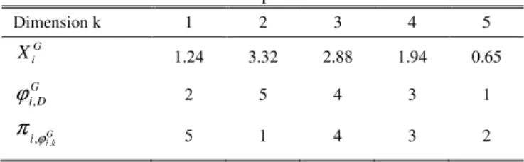
(13)Table 1 illustrates the solution representation of vector XiG for DE. According to the SPV rule, the smallest
dimension value is Xi,5G= 0.65, so ,5=1
G i
ϕ . Therefore dimension k= 5 assigned to be the first job in the permutation. After decoding each vector, the fitness of each vector is evaluated by equation (1).
TABLE I
Solution Representation
Dimension k 1 2 3 4 5
G i
X 1.24 3.32 2.88 1.94 0.65
G D i,
ϕ 2 5 4 3 1
G k i
i,ϕ,
π
5 1 4 3 2B. Initialization
In order to establish a starting point for the optimization process, each decision parameter in every vector of the initial population is assigned a randomly chosen value from within its corresponding feasible bounds:
),
(
0 , L j U j L j ij
X
rand
X
X
X
=
+
−
i= 1,2,…,NPj= 1,2,…,D (14) Where XjL and XjU is considered between [0,4], and rand
represent a uniformly distributed random value that ranges from 0 to 1.
C. Mutation
At every generation G, each vector in the population has to serve once a target vector. For each target vector, a mutant vector ViG is defined by:
)
(
cGG b G
a G
i
X
F
X
X
V
=
+
−
(15)With random indexes a,b,c
∈
NP [7], integer, mutually different, and different to the target vector. F is a user defined constant (also known mutation scaling factor), which is typically chosen from the range (0,2]. Larger values for F result in higher diversity in the generated population and lower values cause faster convergenceD. Crossover
DE utilizes the crossover operation to generate new solutions by shuffling competing vectors and also to increase the diversity of the population. To this end, the trial vector, i.e.,
U
iG=
[
U
1G,i,...,
U
GD]
is formed, where
≤
=
=
Otherwise
X
k
j
or
CR
rand
if
V
U
G i j j G i j G i j , , , (16)In (16), randj is the jth evaluation of a uniform random
number generator with outcome between 0 and 1. CR is the crossover rate constant and is a user-defined parameter within the range [0,1]. Large CR usually increases the convergence rate. K is a random parameter index chosen from the set, which is used to make sure that at least one parameter is always selected from a Vi
G
.
E. Improvement by simulated annealing
Simulated annealing (SA) is a effective optimization algorithm motivated from an analogy between the simulation of the annealing of solid and the strategy of solving combinatorial optimization [17]. In this paper, in order to enhance the exploitation ability of the proposed algorithm, DE is hybridized with a simulated annealing (SA) algorithm. All current solution vectors are improved by using SA.
The applied SA could be briefly introduced as follows: It starts with an initial solution, each solution vector of the current generation, and for each vector a neighbor solution is generated. In the proposed SA, a neighbor vector
[
i Di]
i
N
N
N
=
1,,...,
, for each solution vector Xi isgenerated according to Equation 17.
ρ
×
−
+
=
i j(
Uj Lj)
i
X
rand
X
X
N
(17)
where ρ is used to ensure that parameter values lies inside their allowed ranges in neighbor vector. Let F(X) and F(N) denote the objective function values of the current solution and the neighbor solution, respectively and define ∆ as the
difference between these objectives; that is ∆= F(X) - F(N).
If
∆
≤
0
the neighbor solution is accepted; otherwise it is accepted with probability equal toe
−∆T. Where T is thetemperature parameter such that T > 0. At the beginning, the temperature is set at the initial temperature T0. Then T is
decreased after generations according to the formula T=α×T,
where α is the coefficient controlling the cooling schedule
(0<α<1).
In this study, the T0 is determined by the following
empirical equation:
)
15
.
0
ln(
min max 0F
F
T
=
−
−
(18)Where Fmax and Fmin are the maximum and minimum
objective function values of the initial solution vectors, respectively. Besides, it was found during experiments that the α= 0.8 produce best results. Therefore, it is selected for
the α value.
F. Termination Condition
Termination strategy can be defined differently based on the problem nature, application, or the purpose of the experiment. In this paper, the execution time is used as termination criterion. The pseudo code for the proposed HDE algorithm is given in Fig 1.
IV. COMPUTATIONAL EXPERIMENTS
In this section, extensive experiments are illustrated to evaluate the performance of the HDE to solve the proposed model. The performance of HDE for small-sized instances is compared with optimal solution obtained by the CPLEX software. In order to test the effectiveness and applicability of proposed algorithm to solve large size problems, since the CPLEX requires long computational times, its results are compared with random key genetic algorithm (RKGA) introduced by Bean [14] and the proposed SA explained in section III.
value. Then, crossover operator is applied to each job’s value. In this algorithm, the migration operator replaces the traditional mutation operator. In the migration phase, new individuals are randomly generated and added to the new population. The migration is used to ensure diversity. RKGA is developed for a more highly constrained problem and does not use of a local search. Bean shows the robustness of RKGA by using it to evaluate machines scheduling, vehicle routing, and quadratic assignment problems. This algorithm is implemented according to its description in the literature [14].
Moreover, in order to evaluate the performance of hybridizing SA into the algorithm, the proposed differential evolution (DE) algorithm without local search engine is also considered in the experiments. All these algorithms are coded in MATLAB 7.12.0 and executed on an Intel® Core 2 DuoE4500 at 2.20 GHz with 2.0GB of RAM.
In order to provide a fair comparison between meta-heuristic algorithms, the stopping criteria is set to a maximum elapsed time of (m+n)×Ω, where m is a number of machines, n is a number of jobs, and Ω is a constant coefficient. While different limits could be obtained by different values of Ω, the preliminary tests showed its proper amount as 0.6. Therefore, the computational effort increases as the number of jobs and machines increases.
Data for a set of random instances are randomly generated in small and large sizes. To generate model’s data, such as processing times, Job’s ready times and job’s sizes, the methods presented in [18] is used.
A. Parameter setting
In this section, an experimental study is conducted to determine the best values for the proposed algorithm parameters (i.e., NP, CR, F). The different values considered for each parameter are shown in Table II. Experiment instances are randomly generated by varying the total number of jobs (i.e. n= 20, 40, 60, 80, and 100 jobs) and total number of machines (i.e. m= 2, 4, and 8 machines). For each combination of n×m ten instances are generated for a total of 150.
Statistical experiments are carried out by means of a design of experiments (DOE) [19]. Confidence level is selected as %95 in this study. Table III demonstrates the P -values of these experiments. The performance measure of interest is the total tardiness.
TABLE II
Experimental parameters of HDE
Parameters Level 1 Level 2 Level 3
CR o.5 0.7 0.9
F 0.3 0.5 0.9
NP 100 150 200
Table III shows the HDE algorithm performs better with crossover rate 0.9 than 0.7. In mutation scaling factor (F), it is observed that HDE performs better with mutation rate 0.5 than 0.3. In addition increasing this rate to 0.9 has no significant influence on HDE performance. Increasing population size from 100 to 150 can improve the results significantly, although there is not a significant difference in quality of solution by increasing it from 150 to 200. According to the obtained results, with NP= 100, CR= 0.9, and F= 0.5, proposed HDE yield better solutions.
TABLE III Experimental test results
Parameters Level of experiment P-value
CR 2×1 0.3016
2×3 0.0197
F 2×1 0.0078
2×3 0.3841
NP 2×1 0.0271
2×3 0.2697
B. Comparative evaluation for small-sized instances Experiments with small-sizes instances consist of 15 different size instances, and each size contains 20 randomly generated instances. Therefore, 300 instances are considered in experiments. To evaluate the performance of the proposed algorithm, generated instances are solved, and related results are compared with SA and optimum solutions obtained by the commercial solver CPLEX. The maximum CPU time for the MILP model is set to three hours, that is, if after three hours no optimal solution is obtained, the best current solution is returned.
Regarding the performance measure, the average Relative Percentage Deviation (RPD) is used according to the following equation:
100
×
−
=
sol sol sol
Best
Best
Method
RPD
(19)Where Bestsol is the best known solution obtained after all
experiments carried out through the paper, and Methodsol is
the solution obtained with a given algorithm.
In Table IV, results for small instances are shown for all evaluated methods including the MILP model, proposed HDE, proposed SA, and RKGA. As Table 2 shows, CPLEX is able to obtain the optimal solution of MILP model for all instances with 8, 10, and 12 jobs. For small instances the solutions from the HDE algorithm are also optimal; however, for larger instances (i.e., with 20 jobs) the solution from HDE is better than commercial software. Regarding the rest of the methods, according to Table IV, the best results are provided by proposed HDE, and the results of proposed SA and RKGA is very similar.
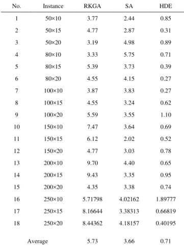
C. Comparative evaluation for large-sized instances In order to test the efficiency of proposed algorithm to solve large size problems, experiments with 18 different sizes jobs are considered. Each size of this problem contains 10 randomly generated instances, and a total of 180
Procedure of hybrid differential evolution
Set parameters: NP, F, CR; Initialize target population;
While stopping criterion is not satisfied Do
Obtain mutant population; Obtain trial population; Evaluation;
Selection;
Update new vectors;
Apply simulated annealing based local search;
End While End
TABLE IV
Comparison results for small-sized instances in terms of RPD
No. Instance MILP RKGA SA HDE
1 6×2 0.00 0.11 0.13 0.00
2 6×3 0.00 0.12 0.15 0.00
3 6×4 0.00 0.17 0.22 0.00
4 8×2 0.00 0.15 0.20 0.00
5 8×3 0.00 0.18 0.26 0.02
6 8×4 0.00 0.21 0.19 0.00
7 10×2 0.27 0.41 0.46 0.02
8 10×3 0.20 0.40 0.49 0.03
9 10×4 0.11 0.54 0.89 0.04
10 12×2 2.24 0.67 0.64 0.06
11 12×3 2.38 1.66 1.88 0.02
12 12×4 2.98 0.82 0.75 0.07
13 15×2 3.51 0.79 0.71 0.04
14 15×3 4.29 0.72 0.62 0.03
15 15×4 5.37 0.85 0.74 0.05
Average 1.42 0.52 0.56 0.03
instances are considered as large size problems. Regarding the performance measure, the RPD is used following Equation 19. In this case MILP model is not tested.
TABLE V
Comparison results for large-sized instances in terms of RPD
No. Instance RKGA SA HDE
1 50×10 3.77 2.44 0.85
2 50×15 4.77 2.87 0.31
3 50×20 3.19 4.98 0.89
4 80×10 3.33 5.75 0.71
5 80×15 5.39 3.73 0.39
6 80×20 4.55 4.15 0.27
7 100×10 3.87 3.83 0.27
8 100×15 4.55 3.24 0.62
9 100×20 5.59 3.55 1.10
10 150×10 7.47 3.64 0.69
11 150×15 6.12 2.02 0.52
12 150×20 4.77 3.03 0.78
13 200×10 9.70 4.40 0.65
14 200×15 9.43 3.35 0.95
15 200×20 4.35 3.38 0.74
16 250×10 5.71798 4.02162 1.89777
17 250×15 8.16644 3.38313 0.66819
18 250×20 8.44362 4.18157 0.40195
Average 5.73 3.66 0.71
In Table V the summary of results for large-sized instances are reported. From the table, it is seen that the HDE exhibits the best performance with the average RPD of 0.71%. As seen in Table V, while the average gap between
the best solution and the HDE is less than 1%, the average gap for the SA and RKGA are less than 4% and 6%, respectively. HDE show a very good performance and provide the best results in most cases.
TABLE VI
ANOVA for average RPD in large-sized instances
Source Degree of freedom
Sum of squares
Mean
square F P-value
Methods 2 2371.76 1185.88 112.53 0.000
Test
Problems 9 87.46 9.72 0.92 0.505
Interaction 18 475.73 26.43 2.51 0.001
Error 540 5690.5 10.54
Total 569 8625.45
To further precisely analysis the results, an analysis of variance (ANOVA) is applied. The ANOVA is shown in Table VI. Confidence level is selected as %95 in this study. It can be seen in Table VI that there are significant differences between the algorithms with p-value very close to zero. Figure 2 present average RPD obtained by these algorithms. From table VI and figure 2 it is obvious that HDE statistically supersedes the other algorithms; also SA is superior to RKGA.
SA RKGA
HDE 6
5
4
3
2
1
0
Methods
M
ea
n
95% CI for the Mean
Fig 2. Method effects plot for average RPD in large size V. CONCLUSION
This paper considered the scheduling batch processing machines in parallel to minimize total tardiness. Also, several practical issues such as unequal job ready times, arbitrary job sizes, and arbitrary job processing times was considered. A mixed integer linear programming (MILP) model was proposed and evaluated to optimally solve this problem using the CPLEX solver. However, the CPU time required by this procedure increases exponentially as the problem size increases and only small-sized instances can be solved optimally using CPLEX. Therefore, a hybrid algorithm based on differential evolution and simulated annealing algorithm (SA), namely HDE, proposed to find optimal or near optimal solution for large size problems. The proposed HDE approach uses smallest position value (SPV) rule based on random key representation to encode solutions, which can convert the job sequences to continuous position values. In addition, calibration of HDE was investigated so that it is ensured that the algorithm performs in a high efficiency.
genetic algorithm (RKGA). The results showed that the solutions from the HDE algorithm were also optimal for these problems. In order to test the applicability of proposed algorithm to solve large-sized instances, 180 instances were generated and the results of HDE were compared with the results obtained by SA algorithm as well as RKGA. The achieved results indicated the effectiveness of the proposed HDE algorithm.
As an interesting future research, a further interesting issue is the consideration of realistic assumption such as machine breakdown in the model. Improving proposed algorithm by combination of other meta-heuristic algorithm is also of interest.
REFERENCES
[1] M. Mathirajan and A. I. Sivakumar, "A literature review, classification and simple meta-analysis on scheduling of batch processors in semiconductor," The International Journal of Advanced
Manufacturing Technology, vol. 29, pp. 990-1001, 2006/07/01 2006.
[2] C. N. Potts and M. Y. Kovalyov, "Scheduling with batching: A review," European Journal of Operational Research, vol. 120, pp. 228-249, 2000.
[3] M. R. Garey and D. S. Johnson, Computers and Intractability; A
Guide to the Theory of NP-Completeness: W. H. Freeman \\&
Co., 1990.
[4] A. H. Kashan, B. Karimi, and M. Jenabi, "A hybrid genetic heuristic for scheduling parallel batch processing machines with arbitrary job sizes," Comput. Oper. Res., vol. 35, pp. 1084-1098, 2008.
[5] P. Y. Chang, P. Damodaran *, and S. Melouk, "Minimizing makespan on parallel batch processing machines," International Journal of
Production Research, vol. 42, pp. 4211-4220, 2004/10/01 2004.
[6] H.-M. Wang and F.-D. Chou, "Solving the parallel batch-processing machines with different release times, job sizes, and capacity limits by metaheuristics," Expert Syst. Appl., vol. 37, pp. 1510-1521, 2010. [7] R. Storn and K. Price, "Differential Evolution \– A Simple and
Efficient Heuristic for Global Optimization over Continuous Spaces,"
J. of Global Optimization, vol. 11, pp. 341-359, 1997.
[8] K. Price, R. M. Storn, and J. A. Lampinen, Differential Evolution: A Practical Approach to Global Optimization (Natural Computing
Series): Springer-Verlag New York, Inc., 2005.
[9] M. F. Tasgetiren, Q.-K. Pan, and Y.-C. Liang, "A discrete differential evolution algorithm for the single machine total weighted tardiness problem with sequence dependent setup times," Comput. Oper. Res., vol. 36, pp. 1900-1915, 2009.
[10] Q.-K. Pan, M. F. Tasgetiren, and Y.-C. Liang, "A discrete differential evolution algorithm for the permutation flowshop scheduling problem," Comput. Ind. Eng., vol. 55, pp. 795-816, 2008.
[11] Q. Niu, T. Zeng, and Z. Zhou, "A novel cultural algorithm based on differential evolution for hybrid flow shop scheduling problems with fuzzy processing time," presented at the Proceedings of the 2011 international conference on Integrated uncertainty in knowledge modelling and decision making, Hangzhou, China, 2011.
[12] F. Liu, Y. Qi, Z. Xia, and H. Hao, "Discrete differential evolution algorithm for the job shop scheduling problem," presented at the Proceedings of the first ACM/SIGEVO Summit on Genetic and Evolutionary Computation, Shanghai, China, 2009.
[13] N. Damak, B. Jarboui, P. Siarry, and T. Loukil, "Differential evolution for solving multi-mode resource-constrained project scheduling problems," Comput. Oper. Res., vol. 36, pp. 2653-2659, 2009.
[14] j. c. Bean, genetics and random keys for sequencing and optimization, 1993.
[15] R. L. Graham, E. L. Lawler, J. K. Lenstra, and R. Kan, "Optimization and approximation in deterministic sequencing and scheduling: a survey," Ann. Discrete Math., vol. 4, pp. 287-326, 1979.
[16] V. Feoktistov, Differential Evolution: In Search of Solutions
(Springer Optimization and Its Applications): Springer-Verlag New
York, Inc., 2006.
[17] S. Kirkpatrick, "Optimization by simulated annealing: Quantitative studies," Journal of Statistical Physics, vol. 34, pp. 975-986, 1984. [18] P. Damodaran, M. C. V, #233, lez-Gallego, and J. Maya, "A GRASP
approach for makespan minimization on parallel batch processing machines," J. Intell. Manuf., vol. 22, pp. 767-777, 2011.