Designing an advanced available-to-promise mechanism compatible with the make-to-forecast production systems through integrating inventory allocation and job shop scheduling with due dates and weighted earliness/tardiness cost

(1)

* Corresponding author.

International Journal of Industrial Engineering Computations 7 (2016) 451–462

Contents lists available at GrowingScience

International Journal of Industrial Engineering Computations

homepage: www.GrowingScience.com/ijiec

Designing an advanced available-to-promise mechanism compatible with the make-to-forecast production systems through integrating inventory allocation and job shop scheduling with due dates and weighted earliness/tardiness cost

Masoud Rabbania*_{, Mina Monshi}a_{, Neda Manavizadeh}b_{Moeen Sammak Jalali}c

a_{School of Industrial Engineering, College of Engineering, University of Tehran, Tehran, Iran} b_{Department of Industrial Engineering, Khatam University,Tehran, Iran}

c_{Faculty of Industrial Engineering & Management Systems, Amirkabir University of Technology- Tehran Polytechnic, Iran}

C H R O N I C L E A B S T R A C T

Article history: Received August 31 2015 Received in Revised Format Septmber 26 2015 Accepted December 8 2015 Available online

December 14 2015

In the competitive business world, applying a reliable and powerful mechanism to support decision makers in manufacturing companies and helping them save time by considering varieties of effective factors is an inevitable issue. Advanced Available-to-Promise is a perfect tool to design and perform such a mechanism. In this study, this mechanism which is compatible with the Make-to-Forecast production systems is presented. The ability to distinguish between batch mode and real-time mode advanced available-to-promise is one of the unique superiorities of the proposed model. We also try to strengthen this mechanism by integrating the inventory allocation and job shop scheduling by considering due dates and weighted earliness/tardiness cost that leads to more precise decisions. A mixed integer programming (MIP) model and a heuristic algorithm according to its disability to solve large size problems are presented. The designed experiments and the obtained results have proved the efficiency of the proposed heuristic method.

Keywords:

Advanced Available-to-Promise (AATP)

Make-to-Forecast (MTF) Batch /real-time mode ATP Jobshop scheduling

Weighted earliness/tardiness cost Inventory allocation

1. Introduction

1.1. Motivation and significance

(2)

1.2.Concepts and literature review

In the literature on operation management, the shortage of a production strategy is obvious for most manufacturing industries. A relatively new simple strategy, called Make-to-Forecast (MTF) has appeared for large engineered equipment which is better than common existing strategies. It can deal with some performance indicators such as fast delivery and customization without increasing costs. This hybrid strategy is a combination of Make-to-Stock (MTS) and Make-to-Order (MTO) strategies in which major product models are produced based on a demand forecast (the part that acts as MTS) by arriving actual orders, proper WIPs would be assigned and modified in order to match the orders’ required characteristics (the part that acts as MTO). MTF strategy is useful for manufacturers producing large and heavy engineered equipment or standalone productions, such as injection molding, pressure vessels, mainframe computers and construction equipment or for aircraft factories or shipyards. In such industries, different products need different operations from the beginning of their own production routes and face an especial challenge that MTF can help considerably from other existing strategies. Due to the importance and the enormous financial flows which exist in the business environment of such industries, any improvement in this manufacturing space can lead to an immense profit. Unfortunately, there are not substantial studies applied MTF strategy. The most prominent studies in this field belong to Akinc and Meredith (2006). They analyzed the appropriate capacity for a MTF production system by presenting a Markov model and investigating orphans, orders leading to a finished unit without a buyer, and rejected orders level. One year later they published another study in which MTF strategy has been thoroughly defined, characterized, structured and illustrated. In that study they also analyzed decision rules for matching partially completed units to incoming orders (Meredith and Akinc, 2007).

Obviously, in this competitive world, customization is one of the most important performance indicators in supply chain, in which suppliers, manufacturers, distributers and retailers try to provide raw materials, make products and finally deliver high quality products to customers by cooperating effectively and efficiently (Beamon, 1998). Therefore, the ability to respond quickly and efficiently in order to satisfy customer demands is considered as a competitive advantage (Weng, 1999). The first step in customization is to respond properly to the agreed order quantity and due date between the customer and the company. The amount of finished goods which is not assigned in a manufactory is called Available-to-Promise (ATP). Implementation of a proper ATP mechanism can enable a company to evaluate the exact production time of the orders. Moreover, it allows using its capacities more efficiently so that orders could be fulfilled on-time (Jeong et al., 2002). ATP's production plan remains in the master schedule in order to support its assignment to the customer orders. In Make-to-Stock (MTS) production systems, ATP can be calculated based on the total inventory of the previous period and total production of the current period (Chen et al., 2001). However, ATP calculation is much more complicated than in ATO, MTO or MTF production systems. Since they contain a higher variety of production, the order quantity is low and due dates are usually less than the required production time. The main purpose of ATP is to satisfy customer orders according to the available resources. Delivering on-time is a major concern of ATP to respond to the customer order. Therefore, an ATP system should have both order promising and order fulfilment abilities. An ATP system should also be able to update the resource consumption dynamically and prioritize customer orders to balance the supply and demand. In such a way, the profit would be maximized (Zhao et al., 2005).

(3)

et al./ International Journal of Industrial Engineering Computations 7 (2016)

commitments. These facts cause researchers to pay attention and investigate under different assumptions. Some authors have studied on ATP form management point of view without presenting quantitative models but some others have tried to define and explain the models in ATP (Schwendinger, 1979; Beamon, 1998; Weng, 1999; Chen et al., 2001; 2002). Fisher (2001) has presented a thorough overview of the studies which had investigated ATP concept. Some have tried to extend its concept and presented new models (Jeong et al., 2002; Xiong et al., 2003; Volling & Spengler, 2011; Cheng & Cheng, 2011). many studies have considered ATP concept with various assumptions to make it applicable in different production environments (Zhao & O.Ball, 2005; Tsai & Wang, 2008; Lin et al., 2010; Chen-Ritzo et al., 2011; Alemany et al., 2013).

Efforts to improve the common ATP model leads to emerge a new type of ATP model, called Advanced ATP which is more compatible with the existing competitive business environment. The exact definition of ATP and Advanced ATP, comparison between them and their applications are completely and comprehensively discussed in a study by Pibernik (2005). Moreover, in this study different classification of Advanced ATPs has been portrayed. One of the most important classifications is to classify Advanced ATP in two groups, batch mode and real-time mode. Each of these has different advantages and applications. In the real-time mode, orders are investigated immediately therefore responsiveness is high. While, in the batch mode, orders which are arrived in a determined interval time would be investigated, simultaneously. Therefore, responsiveness is lower but in this approach a company will not miss more profitable orders. There is no study in the literature which has presented an ATP model for MTF production systems. There is a large portion of industries that work with MTF production system and ATP mechanism can help them improve their production planning. On the other hand, all studies in the literature consider batch mode Advanced ATP (Zhao & O.Ball, 2005; Lin et al., 2010; Cheng & Cheng, 2011) or real-time mode (Volling & Spengler, 2011). Moreover, as the last found gap in ATP literature, most of the reviewed studies have not considered backlog costs. According to these research gaps, in this study we try to design an appropriate ATP model for MTF production systems while trying to combine batch mode and real-time mode and consider holding and tardiness costs. Another immense contribution of this study is to incorporate ATP with job shop scheduling.

In the rest of this paper, section 2 outlines the models and formulations. The proposed heuristic algorithm is explained in section 3. The numerical results are shown in section 4. Finally, concluding remarks are given in section 5.

2. Problem definition and formulation

The main purpose of designing ATP mechanism is to determine whether the firm is able to fulfil arriving orders. A customer order has two characteristics, quantity and delivery date. The role of ATP is to assess newly arrived orders’ characteristics and make decision to accept or reject each order based on the available required sources, materials and production capacity to maximize profit or to minimize costs. In this mechanism, if an order is accepted, its production schedule should be determined. It should be mentioned that in this study, various production routes with different numbers of operations are allowed for different orders and also different options are determined in each workstation to be used and customers should select one of the allowed options for different production processes of their orders.

2.1.Proper Time of Investigating Orders model – PTIO model

(4)

an order in the order basket which has a priority level greater than 0. In Eq. (2) T_Batch, t₀and t_nowrepresent the appropriate time to investigate orders in the order basket, the arrival time of the first order that enters the order basket and the present time respectively.

1

0

tnow

I

i i

OP







(1)

 

1 1

0

1 1

1

1 1

tnow tnow

I I

i i

Batch d _I now _I

i i

OP OP

k k

T t t t

OP OP

k k

 

  _ _  _ _

  _ _  _ _

      

  _ _ __ 

     

 __ _ _ __ _

 

 __ _ _ __ _

  

 ___ _ __ __ _ _

 



 

 

 _

 _

 

(2)

Through this procedure if an order is more profitable, it would get priority level K and be investigated immediately. Also if an order has low importance, it would get low priority level and wait for orders with high priority level to be investigated. Therefore, the company will not lose profitable cases against low profitable ones. On the other hand, each order with any priority level would be answered in t_d units of time to gain customers satisfaction.

2.2.Inventory Allocation and Order Scheduling model – IAOS model

In this model, all the orders entered the order basket will be investigated. The main outputs of this model areX_ijk , YP_ijrsp and YM_ijrsm that explained below as decision variables. Other important outputs derived from decision variables and used in decision makings are TC_i and Ct_ijS that represent total cost of order i and completion time of order i part j respectively.

Indices:

I Number of orders

J Number of units required in each order K Number of WIPs

R Number of operations in production route S Number of workstations

P Number of options in each workstation T Time units

M Number of machines

Decision variables

ijk

X Binary variable equals 1 if kth WIP is allocated to the jth unit of order i and 0 otherwise ijrsp

YP Binary variable equals 1 if the rth operation in production route of the jth unit of order i is done at sth workstation using pth option and 0 otherwise

ijrsm

YM Binary variable equals 1 if the rth operation in production route of the jth unit of order i is done at sth workstation using mth machine in that workstation and 0 otherwise

Parameters

ProCostk Total production cost of kthWIP in previous production steps till now i

Q Number of units required in order i s

ChCost Cost of exchanging an option with another one at sth workstation ijrst

C t Completion time of rth production step of jth unit of ith order at sth workstation at time t i

DueDate Agreed due date of order i

os i

(5)

os i

HoldC t Holding cost of order i per unit of time ijrst

St Starting time of rth production step of jth unit of ith order at sth workstation at time t ijrs

FlowT The period of time in which jth unit of ith order is at sth workstation so that its rth production step would be done

FTCost Holding cost of WIP in production line per unit of time ksr

PRI A binary number that equals 1 if the rth production step of inventory k has been done at sth workstation and 0 otherwise.

isr

PRO A binary number that equals 1 if the rth production step of order i should be done at sth workstation and 0 otherwise.

irp

OPO A binary number that equals 1 if order i require pth option at its rth production step and 0 otherwise

krp

OPI A binary number that equals 1 if pth option is used for rth production step of inventory k and 0 otherwise

ijrst

Z  _{A binary number that equals 1 if}_j_{th unit of}_i_{th order would be at}_s_{th workstation at time}t

to do its rth production step and 0 otherwise ijrs

CCoP Consumption coefficient of jth unit of ith order from option p at workstation s at its rth production step

spt

Opt The amount of material inventory of pth option type at stage s at time t s

M Number of available machines in workstation s s

P Number of available options in workstation s smt

FT  A binary number that equals 1 if mth machine at stage s would not be busy at time t and 0 otherwise

ijrs

PT Processing time of rth production step of jth unit of ith order at stage s The proposed model

1 1 1 1 1 1

1 1 1

( 1) P r os

m ax , 0 os

m in m ax , 0 os

i i i

i

Q K Q R S P

k ijk ijrsp s

j k j r s p

Q S T

ijR st i i

j s t

Q S T

i ijR st i

j s t

ij r s

oC t X Y P C hC ost

C t t D ueD ate T ardC t

D ueD ate C t t H oldC t

S t                   _{ }  _ _ _ _     _ _  _ _       

 

   

 



 



1 1 1 1 1

1 1 1

os t

i

i i O B

Q R S T T

t ijrst i

j r s t t

Q R S

ijrs j r s

t C t t H oldC t

Flow T FT C ost

                               _  _ _ _ _                       



   



  

(3) 1 1 , K ijk k

X i j

  



(4) 1 1 1 i Q I ijk i j X k    



(5)



PRI

_ksr



PRO

_isr





X

_ijk

 

0 i j k s r

, , , ,

(6)

( ) , , , , ,

ijrsp irp krp ijk

YP  OPO OPI X i j k r s p (7)

1 1

, , ,

i

Q I

ijrsp ijrst irs spt

t t i j t t

YP St CCoP Opt r s p t

   

   

(6)

1 1 , , , s s M P ijrsm ijrsp m p

YM YP i j r s

 

 



(9)

1 1 , , , s P T ijrst ijrsp t p

Ct YP i j r s

 

 



(10)

1 1 , , , s P T ijrst ijrsp t p

St YP i j r s

 

 



(11)

0 0

, , ,

T T

ijrst ijrst

t t

Ct t St t i j r s

 

   



(12)

0 0

1, , , ,

T T

ijrst ijrst ijrst

t t

Z  St t t Ct t i j r s

 







  



  (13)

1 1 1 1

1 ,

i

Q

I R S

ijrst ijrsm

i j r s

Z  YM t m

       



(14) 1 , , , T

ijrst smt ijrs t

Z  FT  PT i j r s

   



(15) 0 0 , , , T T

ijrs ijrst ijrst

t t

FlowT Ct t St t i j r s

 





Ct



(22)



0,1,...,



ijrs

FlowT



T

(23)

The objective function given in Eq. (3) minimizes costs including production cost, the cost of exchanging an option used in a WIP that is not suitable for the order matched to that WIP, lateness cost, earliness cost and holding cost of finished goods inventory and also WIPs. In this model none of the orders would be rejected. All orders would be investigated and a delivery date, even so late, will be determined for them. Then according to the information obtained from the model, causes of possible lateness can be recognized. If it can be obviated by out sourcing, partial delivery or other methods therefore order can still be accepted. Constraints (4) and (5) ensure that each order would be allocated to just one WIP and each WIP would be allocated at most to one order. Constraint (6) prevents allocating a WIP to an order while their production routes are not the same. In constraint (7) production steps of the order which should be reworked are determined. Constraint (8) checks that at any time, different orders consumption of different material types in different workstations does not exceed that available material type inventory. Constraints (9), (10) and (11) ensure that for every operation which is determined to be done in constraint (6) in order to complete the orders, a machine at proper workstation must be allocated and also start time and completion time of each operation should be determined. Constraint (12) checks this logical fact that the completion time for each order can’t be before its start time. Constraints (13), (14) and (15) determine the required period of time to complete every operation which is determined to be done in constraint (6) according to their processing time and free times of machines. Constraint (16) calculates period of time at which each order spent on different workstations. Constraints (17)-(23) show the allowed numeric range for binary variables.

3. Heuristic algorithm for inventory allocation and order scheduling (ASH)

(7)

Almeder & Hartl, 2013; Seker et al., 2013; Lamghari & Dimitrakopoulos, 2012; Wang & Zheng, 2013; Kazemi Zanjani et al., 2013; Han et al., 2012) or scheduling (Rudek & Rudek, 2013; Behnamian & Fatemi Ghomi, 2013; Lamghari et al., 2013; Eskandari & Hosseinzadeh, 2013 Wauters et al., 2012; Merdan et al., 2012), just a few studies in the ATP literature have taken advantage of them (Cheng & Cheng, 2011; C-Ritzo et al., 2011; Jeong et al., 2002).

Algoithm 1

Step 1. Find an initial solution

Input orders data (the number of orders=I, production route, processing times and preferred options at each workstation and their different costs per unit) Input WIPs data (Production route and used options at each workstation)

Input machines data (their free times)

Input material data (their availability in the investigated period of time)

Step 1.1. Find proper matches for i=1 to I

Ai= Total processing time×(earliness cost + lateness cost)

end

Ai* = Sort Ai in descending order

for i=1 to I

Find all WIPs with similar production route to Ai*

Calculate the remaining processing time if order Ai* is allocated to each of the found WIPs in previous part

Choose WIP with the least remaining processing time and allocate it to order Ai*

Omit the allocated WIP in previous part from the uncommitted WIPs list

end for

Step 1.2. Schedule the required operations

Z←Determine the proper production route for every WIP allocated to one of the orders to fulfill them X*_←_{Consider the ideal schedule according to Z}_{(it can be feasible or infeasible)}

FY ← According to Zselect one of the required operations of every order to be scheduled first Y← According to the obtained Z and FY organize a sequence of all operations

X← Generate a feasible solution that has the minimum deviation from X*_{according to Y}

Step 2. Improve initial solution

while termination condition does not meet its value do Step 2.0.  ← Generate a random number from 0 to 1

if α < 0.30

Go to step 2.1.

else if 0.3 < α < 0.6

Go to step 2.2.

else

Go to step 2.3.

end

Step 2.1. Local Search 1

a [ β × Number of orders ]

Choose “a” orders randomly

FY’ ← Change the FYvalue for the selected orders

Y’← Apply needed changes in Y

X’← Generate a feasible solution that has the minimum deviation from X*

according to Y’

if X’leads to a better (less) value for the objective function X← X’

FY← FY’ Y← Y’

end if

Go to step 2.0.

Step 2.2. Local Search 2

Y’← Generate a new sequence of operations according to FY

according to Y’

if X’leads to a better (less) value for the objective function X← X’

Y← Y’

end if

Go to step 2.0.

Step 2.3. Global Search

FY’← Change the FY value for all of the orders

Y’ ← Generate a new sequence of operations according to FY’

according to Y’

if X’leads to a better (less) value for the objective function X ← X’

FY← FY’ Y ← Y’

end if

(8)

In this section, in order to solve medium and large size problems we present a two-phase heuristic algorithm. The first phase is designed to generate an initial solution, which includes allocating the most proper WIP to every order to reduce the total weighted remaining processing time and make an initial feasible schedule. The second phase itself includes three steps. The first two steps search local space while the third one probes global space. All of these three steps try to find solutions with less total cost which includes production, earliness, lateness and holding costs. Algorithm 1 presents the procedure of the proposed study.

In this algorithm, orders are first ranked based on their weighted processing times while their weights equal the summation of earliness and lateness costs per unit of time. Then these orders are allocated to the most proper WIP according to their similarity in production route and options in which are used. In this section, all uncommitted WIPs to the investigated order, with similar production route, are collected and put in a list. Then a WIP should be selected from the list, which minimizes the remaining processing time. To select the most proper WIP, the remaining processing time is considered according to the not met workstations and the considered production environment (MTF), for workstations which need to rework – to change the used option – since the used options are not customer’s preferred ones. Finally, this algorithm determines which WIP should be allocated to each order and according to this assignment which operations should be accomplished on the allocated WIP to complete the order. Although considering different options can help algorithms become more realistic especially in assembly lines, it is not considered in previous studies. Finally, to reach an initial solution, the determined operations in the previous section would be scheduled.

The second phrase of this algorithm tries to improve the obtained solution in the first phrase by searching the solution space locally and globally. In the local search procedure, different operations of the same order exchange their positions in the initial solution while, in the global search, every pair of operations owed with different orders would change their positions. In the scheduling part of both phrases, the proposed algorithm, first by disregarding material and machine availability limitations, sets an operation scheduling in which different operations of every order will be done continuously and all of the orders will be finished exactly on time. If this ideal scheduling is possible, we have found the most cost-effective solution. Usually material and machine availability limitations make this obtained ideal solution infeasible. Therefore, this algorithm tries to find a feasible solution by making as less as possible modifications in ideal solution. Therefore, the algorithm needs a sequence of all the operations to determine which operation should be scheduled in the next attempt. However, the sequence of operations must have the feasible solution qualification. For every order, one of its operations would be chosen as the first scheduled operation; it means that the chosen operation appears before other operations of that order in the sequence of operations. If the operations of every order are numbered sequentially, the chosen operation for every order divides the operations of that order in to two categories, predecessor and successor operations. The requirement is that for every order first the successor operations should be appeared in an ascending order then the predecessor operations should be appeared in a descending order. Fig. 1 illustrates the above explanations and shows a possible sequence of operations for the orders.

5.2 3.3 4.3 1.1 2.2 3.2 1.2 5.1 5.3 4.2 2.1 2.3 4.1 5.4 1.3 4.4 3.1

(a)

5.2 3.3 4.3 1.1 2.2 3.2 1.2 5.1 5.3 4.2 2.1 2.3 4.1 5.4 1.3 4.4 3.1

(b)

Fig. 1. A possible sequence of operations

(9)

third operation of order 3 are selected as their first operations to be scheduled. The proposed heuristic method picks up operations based on their sequence and schedules them according to the machines’ free time. Continuous units of time should be allocated to each operation. It means that the pre-emption is not allowed. As the summarizing the results, the output of our heuristic algorithm includes the start time and finish time of every operation and the machine by which the operation would be done.

4. Numerical results

In this section first some sensitivity analysis has been done on the key parameters of the PTIO model, k andt_d. It is apparent that there is a strong relationship between the production capacity and the optimum

values of k andt_d. To prove this assumption, some experiments have been designed. The results are shown in the Table 1 and Table 2. In Table 1, t_dis considered as a fixed value while k varies from 1 to 10. While in table 2, k is assumed constant and the value of t_dvaries. Different capacities are applied according to the summation of machines’ work hours per unit of time (day).

Table 1

Sensitivity analysis on parameter k k value

(t_d 6 days )

Net Profit

Capacity A Capacity B Capacity C

1 6281 6170 2388

3 6541 6395 2654

4 6797 6504 2822*

6 7009 6625 2471

7 7265 6786* 2157

8 7759 6455 1986

9 8106* 6259 1775

10 7934 6086 1542

The quantities 12, 10 and 8 hours are considered respectively for the capacities A, B and C. Net profit is calculated according to the summation of the obtained revenue from all orders minus the total cost which are the cost of production, exchanging an option used in a WIP that is not suitable for the order matched to that WIP, lateness, earliness and goods holding.

Table 2

Sensitivity analysis on parameter t_d

d

t (day)

(k=7)

Net Profit

Capacity A Capacity B Capacity C

1 6895 6167 3354

3 7022 6497 3509*

6 7265 6786* 2157

10 7784 6243 1492

12 8245* 5867 1235

15 7654 5320 976

According to the achieved results it can be concluded that both k and t_dhave similar behaviors via different capacities. In each column of capacities, increasing the value of both variables k and t_dfirst leads to increase in the amount of profit then from one specific point, increasing in the value of k and t_d

(10)

investigate the performance measures in IAOS model and the proposed heuristic algorithm. In this section different performance measures are assessed for different number of orders, machines and WIPs. It is assumed that at least one WIP should exist at the beginning of the production line for every order. The type and the number of processes which are passed for the remaining WIPs are determined randomly with uniform probability. In this section an idle time index is defined to measure performance of the models. This index can take any values from interval [0,1], lower values of this index represent better results since it means the idle time of machines are less sporadic. Therefore, allocating the machines idle time to other orders or maintenance activities is easier.

2 Id

IdleTimeIndex ITC

T

 

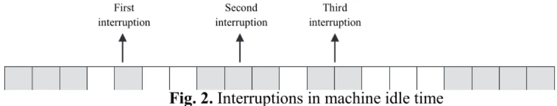
Where Id is the total idle time of machine and T is the investigated horizon time, IT C is a coefficient that equals the number of interruptions in machine idle time. Figure 2 can illustrate this calculation better. The white cell represents the idle time. Id and T equal 7 and 20 respectively and IT C is equal to 3. It should be mentioned that N-M-I represents the number of orders, machines and WIPs respectively. Also processing time in this table points to the remaining required operations which should be done on the allocated WIPs to fulfil the orders. As shown in the table 3, our proposed heuristic algorithm is able to solve even large size problems while GAMS can’t solve them in proper time (600 s). Our heuristic algorithm also can generate solutions with near optimal costs.

Fig. 2. Interruptions in machine idle time Table 3

Experimental results to investigate performance measures in IAOS model

N-M-I

No. of Solved/10

Mean Cost Mean

On-time Orders

Mean Delayed Orders

Mean (Flow Time/ Processing Time)

Mean Idle Time Index

Mean CPU Time (Sec.)

GAMS ASH GAMS ASH GAMS ASH GAMS ASH GAMS ASH GAMS ASH GAMS ASH

10×10×20 10 10 3921 3939 10 10 0 0 1.09 1.12 .152 .326 143 317

10×10×25 10 10 3880 3914 10 10 0 0 1.09 1.10 .157 .342 156 323

15×10×25 8 10 4657 4699 8 7 2 3 1.13 1.18 .096 .304 282 352

15×10×30 7 10 4479 4522 9 9 2 2 1.11 1.15 .118 .312 290 343

20×10×30 5 10 5204 5259 10 9 3 3 1.19 1.25 .068 .259 387 361

20×10×35 3 10 4976 5008 11 11 2 2 1.17 1.21 .076 .277 374 385

20×15×30 2 10 7780 7994 9 8 6 7 1.31 1.43 .099 .321 558 364

20×15×35 0 10 N/A 7851 N/A 10 N/A 7 N/A 1.41 N/A .327 >600 370

20×20×35 0 10 N/A 9546 N/A 8 N/A 8 N/A 1.64 N/A .349 >600 392

20×20×40 0 10 N/A 9266 N/A 8 N/A 7 N/A 1.57 N/A .356 >600 426

Generally, according to the obtained results, this heuristic leads to acceptable performance measures which are related to the orders such as total cost, the number of on-time orders, and the number of delayed orders or the flow time of orders but there is still an observable difference in the results of the defined idle time index. The randomization nature used in scheduling part of the proposed heuristic algorithm enables it to schedule the operations in such a way that more orders would be finished on-time and also overcome the impacts of other factors such as machine availability or bottlenecks. On the other hand, it seems that this characteristic causes sporadic idle time in machines.

Table 4

Comparison of applying randomization procedure in ASH with other scheduling rules

N-M-I Mean Cost Mean

(Flow Time/ Processing Time)

Mean Idle Time Index

SPT EDD CRSPT ASH SPT EDD CRSPT ASH SPT EDD CRSPT ASH

10×10×25 4809 4258 4395 3914 1.25 1.14 1.16 1.10 .073 .132 .069 .342

15×10×30 5369 4877 4980 4522 1.32 1.21 1.24 1.15 .064 .119 .056 .312

20×10×35 5997 5334 5506 5008 1.36 1.24 1.27 1.21 .057 .107 .044 .277

First interruption

Second interruption

(11)

To prove this assumption and also find a way to improve the idle time index, the randomization procedure of the proposed heuristic is replaced with other scheduling rules such as SPT, EDD and CRSPT. As shown in Table 4 both IAOS and ASH models can overcome other models according to the performance measures mean cost and mean (Flow Time/Processing Time). However, applying SPT, CRSPT and EDD leads to obtain better values for idle time index than our proposed models. These results are expected since in our proposed models focus is only on reducing earliness and tardiness costs but this analysis attracts attention to this matter that it can be possible to make a balance between these performance measures through hybrid models which take advantages from different scheduling rules.

5. Conclusion and future works

The main purpose of this study was to design an AATP mechanism compatible with the MTF production systems. According to the special characteristics of this type of production systems, we need detailed information about orders, WIPs, material and machines availability to present a proper AATP mechanism. First, proper WIPs are matched with the orders, then to fulfil the orders, their required remaining processes would be determined and finally the operations would be scheduled to reduce the total cost including the costs of production, holding, earliness and tardiness. The obtained results have proved that our proposed heuristic algorithm is capable to find near optimum solutions even for large size problems.

However, there are still some possible extensions to improve this research. As mentioned in the previous section our heuristic algorithm leads to acceptable values for performance measures such as number of on-time orders, delayed orders or flow time but its results are not good enough for idle time index. Therefore, designing a model which can improve idle time index along with previous performance measures could be valuable. On the other hand, considering other important assumptions such as partial delivery or several manufacturing locations can make the model more realistic.

References

Akinc, U., & Meredith, J. (2006). Choosing the appropriate capacity for a make-to-forecast production environment using a Markov analysis approach. IIE Transactions, 38(10), 847-858.

Meredith, J., & Akinc, U. (2007). Characterizing and structuring a new make-to-forecast production strategy. Journal of Operations Management, 25(3), 623-642.

Alemany, M. M. E., Lario, F. C., Ortiz, A., & Gómez, F. (2013). Available-To-Promise modeling for multi-plant manufacturing characterized by lack of homogeneity in the product: An illustration of a ceramic case. Applied Mathematical Modelling, 37(5), 3380-3398.

Almeder, C., & Hartl, R. F. (2013). A metaheuristic optimization approach for a real-world stochastic flexible flow shop problem with limited buffer. International Journal of Production Economics, 145(1), 88-95. Dictionary, A. P. I. C. S. (2004). Published by the American Production and Inventory Control

Society. Alexandria, VA.

Beamon, B. M. (1998). Supply chain design and analysis: Models and methods. International journal of production economics, 55(3), 281-294.

Behnamian, J., & Ghomi, S. F. (2013). The heterogeneous multi-factory production network scheduling with adaptive communication policy and parallel machine. Information Sciences, 219, 181-196.

Chen, C. Y., Zhao, Z. Y., & Ball, M. O. (2001). Quantity and due date quoting available to promise. Information Systems Frontiers, 3(4), 477-488.

Chien-Yu, C., Zhao, Z., & Ball, M. O. (2002). A model for batch advanced available-to-promise. Production and Operations Management, 11(4), 424.

Cheng, C. B., & Cheng, C. J. (2011). Available-to-promise based bidding decision by fuzzy mathematical programming and genetic algorithm.Computers & Industrial Engineering, 61(4), 993-1002.

(12)

Eskandari, H., & Hosseinzadeh, A. (2013). A variable neighbourhood search for hybrid flow-shop scheduling problem with rework and set-up times. Journal of the Operational Research Society, 65(8), 1221-1231. Figueira, G., Santos, M. O., & Almada-Lobo, B. (2013). A hybrid VNS approach for the short-term

production planning and scheduling: A case study in the pulp and paper industry. Computers & Operations Research, 40(7), 1804-1818.

Fischer, M. E. (2001). Available-to-promise: Aufgaben und Verfahren im Rahmen des Supply-Chain-Management. Roderer.

Han, S. H., Dong, M. Y., Lu, S. X., Leung, S. C., & Lim, M. K. (2012). Production planning for hybrid remanufacturing and manufacturing system with component recovery. Journal of the Operational Research Society, 64(10), 1447-1460.

Jeong, B., Sim, S. B., Jeong, H. S., & Kim, S. W. (2002). An available-to-promise system for TFT LCD manufacturing in supply chain. Computers & Industrial Engineering, 43(1), 191-212.

Zanjani, M. K., Nourelfath, M., & Ait-Kadi, D. (2013). A scenario decomposition approach for stochastic production planning in sawmills. Journal of the Operational Research Society, 64(1), 48-59.

Lamghari, A., & Dimitrakopoulos, R. (2012). A diversified Tabu search approach for the open-pit mine production scheduling problem with metal uncertainty. European Journal of Operational Research, 222(3), 642-652.

Lamghari, A., Dimitrakopoulos, R., & Ferland, J. A. (2013). A variable neighbourhood descent algorithm for the open-pit mine production scheduling problem with metal uncertainty. Journal of the Operational Research Society,65(9), 1305-1314.

Li, X., Baki, F., Tian, P., & Chaouch, B. A. (2014). A robust block-chain based tabu search algorithm for the dynamic lot sizing problem with product returns and remanufacturing. Omega, 42(1), 75-87.

Lin, J. T., Hong, I. H., Wu, C. H., & Wang, K. S. (2010). A model for batch available-to-promise in order fulfillment processes for TFT-LCD production chains. Computers & Industrial Engineering, 59(4), 720-729.

Merdan, M., Moser, T., Sunindyo, W., Biffl, S., & Vrba, P. (2013). Workflow scheduling using multi-agent systems in a dynamically changing environment.Journal of Simulation, 7(3), 144-158.

Toledo, C. F. M., da Silva Arantes, M., De Oliveira, R. R. R., & Almada-Lobo, B. (2013). Glass container production scheduling through hybrid multi-population based evolutionary algorithm. Applied Soft Computing, 13(3), 1352-1364.

Pibernik, R. (2005). Advanced available-to-promise: Classification, selected methods and requirements for operations and inventory management.International journal of production economics, 93, 239-252. Rudek, A., & Rudek, R. (2013). Makespan minimization flowshop with position dependent job processing

times—computational complexity and solution algorithms. Computers & Operations Research, 40(8), 2071-2082.

Schwendinger, J. (1979). Master production scheduling’s available-to-promise. In APICS conference proceedings (Vol. 316, p. 330).

Seker, A., Erol, S., & Botsali, R. (2013). A neuro-fuzzy model for a new hybrid integrated Process Planning and Scheduling system. Expert Systems with Applications, 40(13), 5341-5351.

Volling, T., & Spengler, T. S. (2011). Modeling and simulation of order-driven planning policies in build-to-order automobile production. International Journal of Production Economics, 131(1), 183-193.

Wang, H. F., & Zheng, K. W. (2013). Application of fuzzy linear programming to aggregate production plan of a refinery industry in Taiwan. Journal of the Operational Research Society, 64(2), 169-184.

Wauters, T., Verbeeck, K., Verstraete, P., Berghe, G. V., & De Causmaecker, P. (2012). Real-world production scheduling for the food industry: An integrated approach. Engineering Applications of Artificial Intelligence, 25(2), 222-228.

KEVIN WENG, Z. (1999). Strategies for integrating lead time and customer-order decisions. IIE transactions, 31(2), 161-171.

Xiong, M., Tor, S. B., Khoo, L. P., & Chen, C. H. (2003). A web-enhanced dynamic BOM-based available-to-promise system. International Journal of Production Economics, 84(2), 133-147.