A Memetic Algorithm for a Bi-objective Bus Driver Rostering Problem

A Memetic Algorithm for a Bi-objective Bus Driver

Rostering Problem

Ana Respício, Margarida Moz and Margarida Vaz Pato

A Memetic Algorithm for a Bi-objective Bus Driver Rostering Problem

Ana Respício1,3, Margarida Moz2,3, Margarida Vaz Pato2,3*

1

University of Lisbon, Faculty of Sciences, DI, Bloco C6, 1749-016 Lisboa, Portugal.

respicio@di.fc.ul.pt

2

Technical University of Lisbon, ISEG, 1200-781 Lisboa, Portugal. mmoz;mpato@iseg.utl.pt

3

University of Lisbon, Faculty of Sciences, Centro de Investigação Operacional.

Abstract

The Bus Driver Rostering Problem (DRP) consists of assigning bus drivers to daily duties

during a planning period. The problem considers hard constraints imposed by institutional

and legal requirements. Solutions should as much as possible satisfy soft constraints that

qualify rosters according to either the company’s or the drivers’ interests.

A bi-objective version of the DRP is considered and two models are presented. Due to the

high computational complexity of DRP, this paper proposes the Strength Pareto Utopic

Memetic Algorithm (SPUMA) a new heuristic algorithm specially devised to tackle the

problem. SPUMA genetic component combines utopic elitism with a strength Pareto fitness

evaluation and includes an improvement procedure. Computational results show that SPUMA

outperforms an adaptation of one of the state-of-the-art most competitive multi-objective

evolutionary algorithms, SPEA2.

Keywords: urban transit planning, bus rostering, multi-objective evolutionary algorithm,

memetic algorithm.

*

2

1. Introduction

The rostering problem arises in several operational contexts, such as transport and health care

systems. Ernst et al. extensively surveyed bibliographical references on personnel scheduling

and rostering (Ernst et al., 2004). Rostering of bus drivers, unlike bus crew scheduling, has

not attracted much attention of researchers. Nevertheless, the literature presents different

models for transit crew rostering, namely, network models. Multilevel assignment models

were proposed by Carraresi and Gallo (1984) and Bianco et al. (1992) for a particular bus

driver rostering problem, and by Caprara et al. (1998) focusing on airlines and railway crew

rostering. More recently, Cappanera and Gallo (2004) deal with rostering in an airline

company by using a multicommodity flow model. All these works consider single objective

models.

However, in the rostering context, both the company's and the workers' conflicting interests

must be taken into account which leads to problems with multiple objectives (Landa-Silva et

al., 2004). Consequently, solutions should encompass the trade-off between these two axes.

Multi-objective rostering has been considered in various rostering issues like airline crew

rostering (Lucic and Teodorovic, 1999) or nurse rostering (Moz and Pato, 2007). Catanas and

Paixão (1995) proposed a bi-objective bus driver rostering model based on a set covering

formulation. The model considers the maximum roster duration minimization and

minimization of the total roster cost and the first objective is taken into account implicitly by

introducing side constraints.

Hence, tackling multi-objective rostering problems still remains a challenging issue. On the

other hand, memetic algorithms have been successfully applied to scheduling and timetabling

(Burke and Landa-Silva, 2004). In this work, a bi-objective version of the Bus Driver

Rostering Problem (DRP) is addressed and a new memetic algorithm is proposed and

evaluated.

Section 2 describes a bi-objective optimization problem for a particular set of constraints of a

real problem occurring in a bus company. Two mathematical models are also presented: a

multicommodity multi-objective network flow model, and a preemptive binary goal

programming formulation. Section 3 introduces multi-objective evolutionary algorithms

(MOEAs) and briefly describes one of the most competing MOEA. Section 4 proposes the

3 Computational results are reported and discussed in section 5, where SPUMA is compared

with an adaptation of SPEA2. Finally, section 6 presents some final remarks.

2. The Bus Driver Rostering Problem

2.1 Problem Description

The Bus Driver Rostering Problem is here defined in accordance with the institutional

requirements and norms of a Portuguese urban bus company, besides the Portuguese Labor

Law and the drivers’ union contracts. In the particular situation analyzed, the company

enrolls a fixed set of drivers operating daily from 6:00 a.m. to 12:00 a.m. The DRP thus

consists of assigning a set of drivers to a previously determined set of daily work duties,

during a given period – the rostering period, here 28 days or 4 weeks. A work duty is a daily

working period to be carried out by a single driver on a specific day and it consists of a

sequence of pieces of work, including breaks and idle times. Two types of work duties are

considered: early duties starting between 6:00 a.m. and 3:30 p.m., and late duties starting

between 3:30 p.m. and 12:00 a.m. Every day, each driver is assigned to work in a particular

duty (work duty) or has a day-off (non-work duty). Hence, for each driver, one must produce

a line of work, that is, a sequence of work duties and days-off for the 28 days period. The

solution of the DRP is called a roster - a set of lines of work for all the bus drivers.

Rosters must comply with the conditions and rules imposed by labor union contracts,

institutional and legal requirements which are viewed as hard constraints. These requirements

concern the number of days-off per week, specific days-off per week, a minimum number of

Sundays/weekends-off in the rostering period, a minimum and a maximum number of days

for the length of a rest period, a minimum number of rest hours between two consecutive

work periods and a minimum and a maximum number of consecutive working days, among

others.

The DRP studied in this paper imposes the contracts and company rules through the

following hard constraints:

(h1) each duty must be assigned to one and only one driver;

4 (h3) some drivers must get specific days-off due to planned absences or get all weekends off

due to seniority;

(h4) drivers must rest a minimum of 11 hours between consecutive work duties, that is, early

duties must not be assigned to drivers that worked at a late duty the day before;

(h5) drivers must not work more than 6 consecutive days;

(h6) drivers must get at least 2 days-off each week;

(h7) drivers must get at least 1 Sunday off in each rostering period;

(h8) drivers must work at most 48 hours per week and 176 hours per rostering period.

With regard to company goals, good rosters generally present low cost assignments and small

gaps between each driver's overall scheduled hours and the respective contracted hours per

period. The company must also take into account the interests of the workers. It is well

known that providing satisfaction to workers increases the quality of their performance and

reduces the level of absences. Good rosters for the drivers are usually characterized by equity

in the distribution of Sundays/weekends-off among drivers, equity in the distribution of

overtime work, and equity in the distribution of late duties.

Here, the search for attractive rosters is tackled through soft constraints that rosters should

satisfy, as far as possible:

(s1) equitably distribute overwork among drivers;

(s2) keep the total cost of overwork as low as possible.

Therefore, within the DRP, feasibility of rosters is ensured by the hard constraints, while the

above soft constraints are considered as the two objectives: - objective 1 consists of

minimizing the overtime of the driver with the maximum overtime. Implicitly this also entails

distributing the work equitably among drivers; - objective 2 aims at minimizing the total

overwork cost. This objective favors increasing the workload of the cheaper drivers, while

5 To sum up, given a set of previously known duties, the aim of the DRP is to build a roster for

a 4-week period satisfying hard constraints (h1)-(h8) and optimizing the above mentioned

objectives.

2.2 Mathematical formulations

This problem can be modeled as a multicommodity and multi-objective network flow

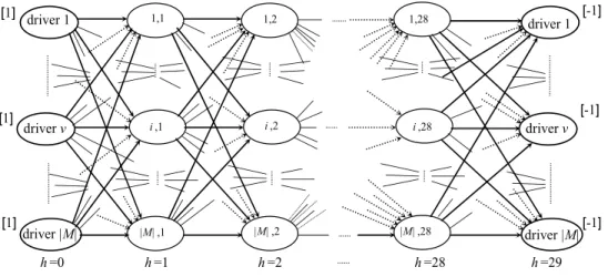
problem with additional constraints defined in a multilayer network.

Consider a network with 28 layers of nodes: one per day of the rostering period (the

day-layers from layer 1 to 28) and 2 additional day-layers of nodes to initialize and finish the rostering

process, layer 0 and layer 29. Taking M as the set of drivers of the company, each layer has

|M| nodes, one per each work duty demanded on that day or per day-off. Each arc in this

network links pairs of nodes of consecutive layers. Figure 1 displays the rostering network.

h=0 h=1 h=2 h=28 h=29

i,1

|M|,1 1,1

i,2

|M|,2 1,2

i,28

|M|,28 1,28

driver 1

driver v

driver |M|

[1]

[1] [1]

[-1]

[-1]

[-1]

driver 1

driver |M|

driver v

Figure 1. The rostering network

In the above multilayer network, a disjoint on the nodes |M|-commodity integer flow from

layer 0 to layer 29, corresponds to a roster for the rostering period. Such a flow must satisfy

all the hard constraints (h1) and (h8). Hard constraints (h1) and (h2) are imposed by the

design of the network and constraints (h5) to (h8) are additional restrictions to be satisfied by

the flow. Constraints (h3) and (h4) are imposed through the definition of costs associated

with the arcs, depending on the driver (commodity) who flows through each arc. In fact, to

avoid the assignment of unfeasible sequences of work duties, on consecutive days, the above

6 The DRP consists of determining a multicommodity integer flow disjoint on the nodes,

through the above defined multilayer network, satisfying additional hard constraints (h5) to

(h8), minimizing total cost and, simultaneously, minimizing the two objectives representing

the quality of the rosters, for drivers and for management.

Next, the second model, a preemptive goal programming approach will be presented in detail.

First the parameters and the sets of data are introduced:

M – set of drivers of the company;

Fv – set of obligatory days-off for driver v, defined by hard constraint (h3), all v∈M ;

cv – cost (in monetary units) of the overtime hour of driver v, all v∈M ;

h h

h T T

T₁ , ₂ , ₃ – sets of early duties, late duties and non-work duties, respectively, of day h,

h=1,…,28;

; 3 2

1h h h

h T T T

T

= ∪ ∪

   = 0 P

p_ihjv allv∈M , all i∈Th, all j∈Th+1, h=1,…27,

where p_ihjv is equal to P if driver v cannot perform on consecutive days, h and h+1, the pair

of duties i and j – due to the rest period of 11 hours imposed by constraint (h4) –, or if driver

v cannot work on either duties i or j because at least one of them is a work duty and h∈Fv,

constraint (h3); and is equal to 0, otherwise;

    = otherwise 0, period rostering previous the of day on worked had driver if , 1 h v ev

h , all v∈M , h=−5,…,0;

tih– length (in hours) of work duty i on day h, all i∈T1h∪T2h, h=1,…,28.

The following variables are used to formulate the DRP:

1 =

x

vihj if driver v performs duty i on day h and duty j on day (h+1)or not (=0);

1 =

y

v_ih if driver v performs duty i on day h or not (=0);

0

1≥

+

δ

– slack for the maximum overwork per driver (in hours);

0

2 ≥

+

δv

7 The preemptive binary goal programming formulation follows:

Min _{

43 42 1 4 4 4 3 4 4 4 2 1 f f f v h M v h v v ihj M

v iT jT h v

ihj

x

λ

λ

c

p

λ

h h 2 1 0 1 2 28 1 2 1 1 27 1

0

δ

δ

+ ∈ = + ∈ ∈ ∈ =

∑ ∑

∑ ∑ ∑ ∑

+ + + (1) subject to: 1 =

∑

∈M v v ih

y

, all i∈Th, h=1,…,28 (2)

1 =

∑

∈Th i

v ih

y

, all v∈M , h=1,…,28 (3)

6 6

0 _3, ,

≤

∑ ∑

= ∉ ₊ + l i v l h i

T hl

y

, all v∈M , h = 1,…,22 (4)

6 6 1 0 3 ≤ +

∑ ∑

∑

+ = ∉ = h l i v il h l v l T l

y

e

, all v∈M , h = −5, …, −1, 0 (5)

2 7 1 ) 1 ( 7 3 ≥

∑

∑

+ − = ∈ l l h i v ih T h

y

, all v∈M (6)

1 4

1 ,7

7 , 3 ≥

∑ ∑

= ∈ l i v l i T l

y

, all v∈M (7)

48 7 1 ) 1 (

7 _{1 2}

≤

∑

∑

+ −

= ∈ ∪

t

y

v ih l l h i ih T T h h

, all v∈M , l = 1,…,4 (8)

176

28

1 _{1 2}

≤

∑

∑

= ∈ ∪

t

y

v ih h i

ih

T Th h

, all v∈M (9)

∑

+ ∈ = 1 h T j v ihj v ih

x

y

, all v∈M , all i∈Th , h = 1,…,27 (10)

∑

− ∈ − = 1 , 1 , h T j v i h j v ih

x

y

, all v∈M , all i∈Th , h = 2,…,28 (11)

8 1 2 1 ≤ − ∑ + ∪

∈_{T T} t y δ

v ih

i _{h h} ih

, all v∈M , h = 1,…,28 (12)

8 2 2 1 ≤ − + ∪

∈

∑

δ

v h v ih i ih y T T t h h

, all v∈M , h = 1,…,28 (13)

0,1 =

x

vihj , allv∈M , all i∈Th , all j∈Th+1, h = 1,…,27 (14)

0,1 =

8 0

1+≥

δ (16)

0

2 ≥

+

δv

h , all v∈M , h = 1,…,28. (17)

At the highest priority level, the minimization of the objective function in (1), by taking λ₀

equal to a big penalty associated to the function f₀, imposes rostering hard constraints (h3)

and (h4). At the second level of goals, the coefficients λ1 and λ2∈ (λ1, λ2∈[0,1]) associated to

functions f₁ and f₂ are forcing the satisfaction of the two soft constraints, (s1) and (s2),

respectively.

The first two sets of equalities (2)-(3) impose the hard constraints (h1) and (h2) and the

following set, (4)-(5), hard constraints (h5). Inequalities (6)-(7) are related to the constraints

(h6) and (h7) and, finally, constraints (h8) are forced by (8)-(9).

The linking constraints (10)-(11) state the coherence of variables y and x and inequalities

(12)-(13) define the slack variables used to formulate the second level goals of the problem.

Finally, conditions (14)-(17) impose the domains of the variables.

The DRP above formulated is an NP-hard problem as proved in Moz and Pato (2007) for a

similar rostering problem regarding nurse rostering.

Moreover, the computational experience shows the difficulty in solving some real driver

rostering problems to reach optimality and even to obtain feasible solutions. In fact, using

software CPLEX 10.2 optimizer, for the goal programming model above described, exact

solutions were obtained only for some of the smallest test instances described in section 5.

This experience motivated the development of evolutionary heuristics that in general are well

equipped to deal with high complexity problems.

3 Multi-objective evolutionary algorithms

3.1 Context

Early approaches to multi-objective problems consist of combining the objectives under

consideration on a single objective function by assigning weights to the objectives and

optimizing that function. However, these approaches are not able to reach some of the

9 problems is that a single point in the objectives’ space usually corresponds to several

solutions in the space of variables. In practice, this multiplicity of equivalent solutions should

be taken under consideration, as decision-makers aim at analyzing other implicit criteria often

enclosed and hard to translate into mathematical models. In general, optimizing methods lose

this multiplicity of equivalent solutions. On the contrary, Multi-Objective Evolutionary

Algorithms (MOEAs) show ability for dealing with the combinatorial complexity providing,

at the same time, good approximations of the solution set as well as taking into account the

multiplicity of equivalent solutions.

In the last decades, diverse MOEAs have been proposed in the literature. Among the most

competing state of the art MOEAs are Strength Pareto Evolutionary Algorithm (SPEA2)

proposed by Zitzler et al. (2002) and Non-dominated Sorting Genetic Algorithm (NSGA-II)

proposed by Deb et al. (2000). In both cases, some common features are used: individuals are

evaluated under the concept of Pareto dominance, as defined in Goldberg (1989); and elitism

is implemented by keeping potentially non-dominated individuals, found so far during the

genetic search, in an external population (the archive).

3.2 SPEA2

In the following, a brief description of SPEA2 will be given to simplify reading of the MOEA

under proposal.

The most remarkable aspect of SPEA2 is its fine-grained fitness assignment scheme, which is

based on dominance counting. Let Pop denote the population set and Arc denote the archive.

Then, the strength of individual i, S(i), is given by the number of individuals, both in the

population and in the archive, that are dominated by i. Hence,

{

j j Pop Arc i j

}

i

S()= | ∈ ∪ , f , where if j means that individual i dominates j , i.e., i

performs better than j in at least one of the objectives and does not perform worst on the

remaining. The raw fitness of an individual i, R(i), is given by the total strength of

individuals dominating i, =

∑

_{∈ ∪}

i j Arc Pop

j S j

i R

f

, ( )

)

( . An individual with a null raw fitness

value is a potentially non-dominated solution for the multi-objective problem. For problems

with a large number of solutions in the Pareto front, especially where variables have

continuous domains, a diversity factor should be added to the raw fitness, as the latter alone

10 density factor D(i)=1

(

σ_ik +2

)

, where σ_ik is the distance of i to it k-th nearest neighbor and

Arc Pop

k= + penalizes individuals in the more crowded regions. Finally, the fitness of

individual i is given by F(i)=R(i)+D(i). Hence, potentially non-dominated individuals are

assigned fitness values in the interval [0,1], while the others have fitness value greater than 1.

SPEA2 includes a special truncation procedure to manage the introduction of potentially

non-dominated individuals in the archive.

In a first approach to DRP an adaptation of SPEA2 (ASPEA2) was developed (Moz et al.,

2007). It was compared with a utopic genetic heuristic and has shown ability to attain a better

coverage of the Pareto front, while the utopic genetic heuristic found more diversity. Taking

into account these two aspects, a new MOEA combining the best features of both algorithms

was developed and will be described in the following section.

4 Strength Pareto Utopic and Memetic Algorithm (SPUMA)

4. 1 SPUMA general features

As defined in section 2.1 the DRP under consideration is a bi-objective problem for which the

Strength Pareto Utopic and Memetic Algorithm (SPUMA) was specially devised.

Algorithm 1 describes the main steps of SPUMA.

The algorithm applies a local search heuristic within a genetic evolution scheme combining

utopic elitism with a strength Pareto fitness evaluation. The basic genetic components

include, in each generation, a fixed dimension population, and archive, where each individual

is characterized by a pair of chromosomes. In this pair, one of the chromosomes represents

the list of duties and the other the list of drivers, and both are coded by integer vectors.

SPUMA was developed on the basis of SPEA2 and additionally considers the insertion of a

utopic individual and the potentially lexicographic individuals in the mating pool of each

generation. The utopic individual is associated with a well fitted solution which is probably

unfeasible. In each generation, each lexicographic individual is related to a feasible solution

that is potentially the most adapted to optimize one of the objectives as it corresponds to one

of the outer approximate front points in the objectives’ space. Here, as the DRP under study

11 Algorithm 1 Strength Pareto Utopic and Memetic Algorithm (SPUMA)

Step 1. Initialization: Set the number of generations t=0. Create an initial population Pop ₀

with |Pop| randomly generated individuals. Create an empty archive Arc₀. Insert

individuals corresponding to the lexicographic points lex1 and lex2 and the utopic

individual into Arc₀.

Step 2. Fitness assignment: For each individual i∈Pop_t∪Arc_t compute fitness value F(i).

Step 3. Environmental selection: Update individuals corresponding to lexicographic points, if

needed, and insert them as well as the utopic individual in the archive of the next

generation, Arc_t+1. Sort the remaining individuals in Pop_t∪Arc_t by increasing order

of fitness. Fill Arc_t+1 with the first |Arc|-3 individuals in the obtained ordering.

Step 4. Termination: If the maximum number of generations has been reached, stop and set

the solution equal to the set of non-dominated individuals in Arc_t.

Step 5. Mating selection: Build a mating pool by selecting individuals in Pop_t∪Arc_t by

binary tournament with replacement.

Step 6. Variation: Perform crossover and mutation over the mating pool giving rise to the

population of the next generation Pop_t+1. Increment current generation t=t+1.

Return to step 2.

The initial population is randomly generated and a given number of warm-up generations are

performed to attain feasibility.

At each generation, a decoder procedure, described in Algorithm 2, transforms each pair of

chromosomes into a DRP solution, allowing for its evaluation.

Because the decoder does not ensure feasibility, rosters that do not satisfy all the hard

constraints get a penalization in both objectives’ values and, as a result, these individuals are

less prone to be chosen for reproduction. The penalization value – a big real non-negative

value – is the same for all the situations where unfeasibility occurs, without differentiating

12 Algorithm 2 Decoder procedure

Step 1.All work duties are set non-assigned. For each day of the rostering period, all drivers

are set free.

Step 2.Select the next non-assigned work duty and search for a driver free in the

corresponding day to assign it ensuring satisfaction of the hard constraints.

If such a driver exists, perform the assignment and mark both elements (work duty

and driver) as non-free.

Step 3.Repeat step 2 while it was possible to assign the current work duty and there are free

work duties.

Step 4.If all work duties were assigned (a feasible solution was found), compute the two

objective values of the solution.

Otherwise (the solution is unfeasible), assign a big value to both objective values,

penalizing the individual.

In previous experience with ASPEA2, it was observed that a single run of the algorithm was

quite ineffective in generating wide spread fronts. This can be explained by the fact that the

problem is discrete and instances have a small number of efficient solutions, leading to a poor

exploration of the SPEA2 diversity component. Consequently, in SPUMA, fitness is

computed without the density factor D, meaning that the fitness of individual i is given by its

raw fitnessF(i)=R(i).

A mating pool is built using binary tournament. Selection is performed considering the

individuals in the archive and those in the population. Note that, SPEA2 also use binary

tournament but only over the archive.

Recombination is done by applying the order crossover operator (OX) on each pair of

chromosomes. The mutation operator is the swapping operator which for each chromosome

in a pair swaps the position of two alleles chosen at random. Both genetic operators act in the

same way and independently on the two types of chromosomes of individuals selected from

13 As mentioned above, SPUMA considers elitism and utopia. Besides the elitism of SPEA2,

the utopic individual and the lexicographic individuals, previously determined, are included

in the archive and are considered for the reproduction process, at each generation. Whenever

a better approximation of an outer point of the true Pareto front is found, the corresponding

lexicographic individual is updated.

4.2 Computing the lexicographic and the utopic individuals

The lexicographic and utopic individuals are previously computed by a single objective

evolutionary algorithm that runs before SPUMA. Algorithm 3 describes the generic

procedure where the specificity of the individual under search is mainly oriented by the

fitness function. As in the main component of SPUMA, Algorithm 3 considers a fixed

dimension population of Pop individuals, coded in the same way. Elitism is implemented by

keeping record of the best individual found so far, which is inherited by the population of the

next generation.

Algorithm 3 Single objective evolutionary algorithm to obtain the lexicographic lexj

individual

Step 1. Initialization: Set the number of generations t=0. Create an initial population Pop ₀

with |Pop| randomly generated individuals. Initialize best individual with an

individual randomly chosen among the population.

Step 2. Fitness assignment: For each individual i∈Pop_t search for the corresponding DRP

solution using the decoder and compute the fitness value according to the objective

function f_j(i). Update best individual.

Step 3. Mating selection: Build a mating pool by selecting individuals in Pop_t by binary

tournament with replacement.

Step 4. Variation: Perform crossover and mutation over the mating pool giving rise to the

population of the next generation Pop_t+1.

Step 5. Termination: If the maximum number of generations has been reached, stop and set

the solution equal to the best individual.

14 At the end, the solution corresponding to the best individual is adopted for the purpose under

consideration. The above algorithm runs three times, in each one minimizing a given fitness

function.

Each of the lexicographic individuals is obtained by considering as fitness function the value

of the corresponding objective. In step 1, the best individual is initialized with a randomly

chosen one. Here, the decoder considers all the hard constraints of the DRP, forcing

feasibility of the corresponding solutions.

Algorithm 3 runs once again to obtain the utopic individual. However, in step 1, instead of

choosing at random an individual from the population, the best individual is initialized with

one of the lexicographic. In step 2, the decoder only considers the hard constraints (h1), (h2)

and (h4), all the other hard constraints being relaxed. This produces solutions that may be

unfeasible with respect to the original problem. Here, the fitness function is such that one

tries to bring the points as close as possible to the origin. As the objectives have different

scales, a standardization brings objective values to the interval [0,1]. Let lex1=(lex₁1,lex1₂)

and lex2 =(lex₁2,lex₂2) denote the lexicographic points. Hence, lex₁1 and lex₂2 approximate

the optimum values of (s1) and (s2), respectively. The individual i, associated with point

)) ( ), (

(f1 i f2 i in the objective space, is assigned a fitness value

(

) (

₁

)

2

2 2

2 2 1

1()/ ()/

)

(i f i lex f i lex

F = + that measures the Euclidean distance of

(

1

)

2 2

2 1

1(i)/lex , f (i)/lex

f to (0,0). The procedure minimizes F(i) searching for a point lying

inside the first quarter of the circle of radius one centered at the origin, as illustrated in Figure

2. It should be noticed that the utopic does not necessarily dominate the lexicographic.

Figure 2. Transformation of the objectives values into the region

[ ] [ ]

0,1 × 0,1 )

,

( 12

1 1 1 lex lex lex = ) ,

( 22

2 1 2 lex lex lex =

(ut1,ut2)

ut=

(

1

)

2 2 2 1 1/lex ,ut /lex

ut

1

f f₁

2

f f₂

) , (lex₁1 lex₁2 1

2 1 1 2 ) , 1

15 4.3 Local search

The local search component tries to find a feasible solution if at a given generation the only

individuals in the population(s) that correspond to feasible solutions are the lexicographic. In

that case, the improvement procedure presented in Algorithm 4 is applied to a randomly

selected individual. It is a constructive heuristic working alike the decoder, but ensuring

feasibility by searching for better local neighbors.

Algorithm 4 Improvement decoder procedure

Step 1.All work duties are randomly ordered and considered not assigned. For each day of

the rostering period, all drivers are set free.

Step 2.Select the next non-assigned work duty and search for a driver free in the

corresponding day to assign it ensuring satisfaction of the hard constraints.

If such a driver exists, perform the assignment and mark both elements (work duty

and driver) as non-free.

Step 3.Repeat step 2 while it was possible to assign the current work duty and there are free

work duties.

Step 4.If all work duties were assigned (a feasible solution was found), compute the two

objective values of the solution. Stop.

Step 5.It was not possible to assign the current duty, say A, to any driver.

If A is not in the first position, then

Backtrack to the last work duty already assigned, say B.

Set work duty B non-assigned and set the driver assigned to it free for that day.

Insert A in the position of B, pushing B and its successors one position forward.

Go to step 2.

16 The procedure stops when all the duties are assigned or when it reaches a duty that cannot be

assigned. In the latter case, the pair of chromosomes still represents an unfeasible solution,

and this leads to stopping SPUMA main cycle.

The next section describes the computational experiments and presents their respective

results. The experiments aim at comparing the performance of SPUMA against those

obtained with the adaptation of SPEA2 (ASPEA2).

5 Computational tests

5.1 Description of the instances

Each instance of DRP is defined by the following data:

• number of drivers;

• last day-off and last work duty for each driver in the previous roster;

• set of work duties per day (week days and weekend);

• for each work duty, the beginning time and the duration.

Computational tests with the evolutionary algorithms were performed over data obtained

from instances of the Integrated Multi-depot Vehicle and Crew Scheduling Problem (VCRP)

solved by Mesquita et al. (2006). The first set includes 10 DRP instances resulting from the

solution of 80 trips VCRP-instances. These DRP instances include 504 work duties for the

rostering period on average. The 11 DRP instances in the second set come from solutions of

100 trips VCRP-instances (DRP instances with 620 work duties on average). All the VCRP

instances are benchmark random instances provided by Huisman et al. (2005). Finally, the

third set includes 15 DRP instances based on real data from the Portuguese urban bus

company under study. In this set, the average number of work duties is 643 on average.

For all these problems the number of drivers considered is 70 and the other data came from

the files of the company.

5.2 Implementation details

Concerning the parameters’ values, for both genetic algorithms, the probability of

reproduction was set to 0.8, while the mutation probability was set to 0.2. As stopping

condition a maximum number of 2000 generations is considered. Feasibility is checked at

17 individuals is achieved by performing 500 generations of the Algorithm 3 described in

section 4. The utopic is obtained by performing 500 generations of the same algorithm.

In all the experiments Pop =40 and Arc =10.

Results for each algorithm were obtained by performing 10 runs and, at the end, computing

the final approximation of the Pareto front by merging the fronts obtained in all the single

runs and extracting the non-dominated individuals.

Both algorithms were coded in C language and the experiments were made on a Pentium 4

processor running at 3.2 GHz and using 1 GB of RAM.

5.3 Performance metrics

In the context of this application, rostering has been done manually by human planners that

will remain in charge of choosing the solution to implement. Furthermore, they are interested

in examining a variety of optimal solutions. Therefore, the cardinality of the Pareto front

approximation is one of the performance metrics used to evaluate SPUMA regarding

diversity. This metric, also known as front occupation was first used by Veldhuizen (1999).

The experiments evaluate the number of potentially non-dominated individuals obtained in

the populations (main population and archive) of the last generation. Its counterpart in the

design space will also be evaluated through the corresponding number of potentially efficient

solutions.

As mentioned above, in previous experience with ASPEA2, it was observed that a single run

of the algorithm was quite ineffective in generating wide spread fronts. Consequently, the

front spread, introduced by Zitzler (1999), will also be evaluated.

As the individuals under evolution may correspond to unfeasible DRP solutions, the number

of feasible solutions in the population of the last generation is measured. Additionally, the

ratio of potentially efficient solutions over the number of feasible solutions is also evaluated,

the feasibility rate. This metric is specially devised for the MOEAs under assessment as it

aims at evaluating the ability to produce feasible solutions.

For each set of instances the analysis of the results is reported and discussed through two

perspectives. Firstly, the above metrics will be computed to evaluate average results per run

18 (FAP) obtained by all the performed runs of each algorithm per instance of the problem.

This set is obtained by merging the potentially non-dominated points in all these runs and,

afterwards, eliminating all the dominated points. Again, the front occupation of FAP will be

analyzed as well as the front spread.

Finally, a measure of the relative strength of FAP is used for pair-wise comparing the two

algorithms. Consider FAP1 and FAP2 two approximations of the Pareto front. The relative

strength of FAP1 over FAP2 is given by

{

i∈FAP1:∃i'∈FAP2,ifi'

}

FAP1, that counts

the number of points in FAP1 that dominate at least one point in FAP2 over the total

number of points in FAP1. A similar metric within the solutions’ space was proposed in

Zitzler and Thiele (1999).

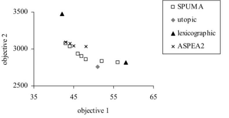
Figure 3 presents graphically an example of typical final Pareto front approximations for one

instance. The squares represent the SPUMA solution, the triangles are the two initial

lexicographic solutions, inserted in the population of generation zero, the diamond represents

the utopic solution, and, the solution obtained by ASPEA2 is represented by crosses.

2500 3000 3500

35 45 55 65

objective 1

o

b

jectiv

e 2

SPUM A

utopic

lexicographic

ASPEA2

Figure 3. Final approximations of the Pareto front obtained by SPUMA and ASPEA2

In this example, SPUMA was able to generate a wider spread (261 against 54) and diverse

front, as the lexicographic individuals work like attractors to the true Pareto front outer

solutions, while the utopic has provided genetic material to generate better solutions.

Additionally, SPUMA attained a better front occupation (8 against 4) and, in particular, the

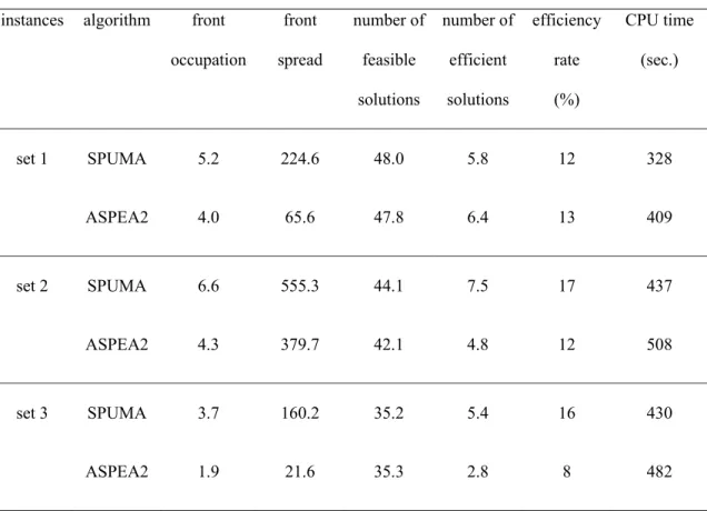
19 5.4 Numerical results

Table 1 reports the average results obtained per run. For each run with a specific instance, the

metric values were evaluated and averages per each set of instances were computed. The

table is divided into three sections, showing the results for both SPUMA and ASPEA2 over a

given set. The columns refer to: the average front occupation; the average front spread; the

average number of feasible solutions; the average number of potentially efficient solutions;

the average efficiency rate (in percentage); and the total CPU time in seconds, respectively.

Table 1 Average results per run

instances algorithm front

occupation

front

spread

number of

feasible

solutions

number of

efficient

solutions

efficiency

rate

(%)

CPU time

(sec.)

set 1 SPUMA 5.2 224.6 48.0 5.8 12 328

ASPEA2 4.0 65.6 47.8 6.4 13 409

set 2 SPUMA 6.6 555.3 44.1 7.5 17 437

ASPEA2 4.3 379.7 42.1 4.8 12 508

set 3 SPUMA 3.7 160.2 35.2 5.4 16 430

ASPEA2 1.9 21.6 35.3 2.8 8 482

The CPU time required to pre-compute the utopic and the lexicographic individuals within

SPUMA was averaged over the number of runs and added to the time value presented.

The front occupation and front spread values show that a single run of SPUMA, on average,

was able to reach more diverse front approximations for all sets of instances, than ASPEA2.

Regarding the front occupation, about 50% more solutions were found. In all cases, the

number of efficient solutions is higher than the front occupation confirming the capacity of

20 rate shows that SPUMA was always able to produce a larger number of equivalent solutions.

Both algorithms revealed a similar performance in their capacity to obtain feasible solutions.

Concerning differences between the sets, the real based instances (set 3) presented smaller

front occupation values for both algorithms. It is interesting to notice that in this case, the

number of feasible solutions was much smaller than that of the other sets. This happens

because in set 3 there are very difficult instances, where solutions show a larger occupancy of

the drivers.

Finally, SPUMA also presents lower CPU time, although it outperformed ASPEA2 in

solution quality. This is explained by the suppression of the density factor in the fitness

function, which was rather time consuming though useless for this particular application.

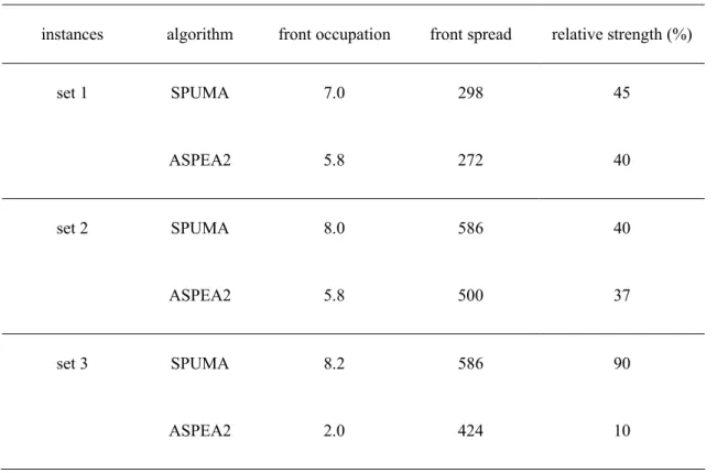
Table 2 displays the average results for the final approximations of the Pareto front. Again,

the table is divided into three sections, each of which reporting algorithms’ results over a

given set. The columns present, respectively, average values of the front occupation, the front

spread, and the relative strength of the two algorithms (in percentage).

Table 2 Average results from final approximations of the Pareto front

instances algorithm front occupation front spread relative strength (%)

set 1 SPUMA 7.0 298 45

ASPEA2 5.8 272 40

set 2 SPUMA 8.0 586 40

ASPEA2 5.8 500 37

set 3 SPUMA 8.2 586 90

21 The results in Table 2 show that SPUMA clearly outperforms ASPEA2. The values of front

occupation and front spread are always greater for SPUMA, revealing its superiority in

producing solutions with diversity. This difference is of particular evidence for the real based

instances, where the front occupation is four times greater than the one of ASPEA2.

Concerning the relative strength, SPUMA has presented greater values than ASPEA2,

meaning that, on average, it was able to achieve better final approximations to the Pareto

front. Although this superiority is not relevant for sets 1 and 2, for the real-based instances

SPUMA reached a relative strength of 90% over ASPEA2 against the relative strength of

10% of ASPEA2 over SPUMA.

Comparing the values for the front occupation and front spread in the two tables, it is evident

that the final approximations were much better than those obtained per run. This reveals that

a single run of the algorithm is not sufficient to produce an adequate approximation of the

true front, in terms of diversity and coverage. Again, the difficulty of instances in set 3

explains a larger difference between these values, as for SPUMA the final front occupation is

8.2 against 3.9 per run, and the final front spread is 586 against 160 per run.

6 Conclusions

This paper is devoted to a new memetic evolutionary heuristic for a Bus Driver Rostering

Problem. This specially devised algorithm, SPUMA, is compared with an adaptation of a

standard procedure, SPEA2, in three sets of instances obtained from real and randomly

generated data and taking into account Law and institutional rules for a Portuguese urban bus

company. The innovation of SPUMA consists of introducing in the mating pool of each

generation a utopic individual and two lexicographic individuals, one for each objective of

DRP, both previously computed by a single objective evolutionary algorithm.

The computational results revealed that the strategy adopted in SPUMA, though conceptually

simple, is quite effective at improving the approximation to the Pareto front as compared with

the most competitive MOEAs. Besides, it is inexpensive in terms of computational effort.

The proposed approach seems to be adequate for real-life applications as it provides planners

with a wide variety of potentially efficient rosters that are difficult to obtain manually and, in

22 Moreover, SPUMA may be easily adapted to other hard combinatorial optimization

problems, eventually with more than two objectives, occurring in scheduling or other

contexts. In fact, as the constraints are considered, in the algorithm, as rules to be imposed

through the decoder, additional constraints can be easily introduced.

References

Bianco, Lúcio, Maurizio Bielli, Aristide Mingozzi, Salvatore Ricciardelli, and Massimo

Spadoni. (1992). “A Heuristic Procedure for the Crew Rostering Problem,” European Journal

of Operational Research 58, 272:283.

Burke, Edmund and Dario Landa-Silva. (2004). “The Design of Memetic Algorithms for

Scheduling and Timetabling Problems,” Studies in Fuzziness and Soft Computing 166,

289-312.

Cappanera, Paola and Giorgio Gallo. (2004). “A Multicommodity Flow Approach to the

Crew Rostering Problem,” Operations Research 52, 583-596.

Caprara, Alberto, Paolo Toth, Daniele Vigo, and Fishetti Matteo. (1998). “Modeling and

Solving the Crew Rostering Problem,” Operations Research 46, 820:830.

Carraresi, Paolo and Giorgio Gallo. (1984). “A Multilevel Bottleneck Assignment Approach

to the Bus Driver’s Rostering Problem,” European Journal of Operational Research 16,

163-173.

Catanas, Fernando and José Paixão. (1995). “A New Approach for the Crew Rostering

Problem.” In Daduna, Joachim, Isabel Branco, and José Paixão (eds.), Computer Aided

Transit Scheduling. Lecture Notes in Economics Mathematical Systems 430. Springer.

267-277.

ILOG (2006). ILOG CPLEX 10.2, User's Manual. Incline Village, NV: ILOG CPLEX Div.

Deb, Kalyanmoy, Samir Agrawal, Amrit Pratap, and T. Meyarivan. (2000). “A Fast Elitist

Non-dominated Sorting Algorithm for Multi-objective Optimization: NSGA-II.” In

Schoenauer, Marc et al. (eds.), Parallel problem Solving from Nature – PPSN VI. Lecture

23 Ernst, Andreas, Houyuan Jiang, Mohan Krishnamoorthy, Bowie Owens, and David Sier.

(2004). “An Annotated Bibliography of Personnel Scheduling and Rostering,” Annals of

Operations Research 127, 21:144.

Goldberg, David E. (1989). “Genetic Algorithms in Search, Optimization and Machine

Learning.” Addison-Wesley, Reading.

Huisman, Dennis, Richard Freling, and Albert Wagelmans. (2005). “Multiple-Depot

Integrated Vehicle and Crew Scheduling,” Transportation Science 39, 491:502

Landa-Silva, Dario, Edmund Burke, and Sanja Petrovic. (2004). “An Introduction to

Multiobjective Metaheuristics for Scheduling and Timetabling.” In Gandibleux Xavier, Marc

Sevaux, Kenneth Sörensen, and Vincent T’Kindt (eds.), Metaheuristics for Multiobjective

Optimisation. Berlin: Springer. 91-129.

Lucic, Panta and Dusan Teodorovic. (1999). “Simulated Annealing for the Multi-objective

Aircrew Rostering Problem,” Transportation Research Part A 33, 19:45.

Mesquita, Marta, Ana Paias, and Ana Respício. (2006). “Branching approaches for the

integrated vehicle and crew scheduling,” Working paper 9/2006, CIO, University of Lisbon

(submitted) 18 pp.

Moz, Margarida and Margarida Pato. (2007). “A Genetic Algorithm Approach to a Nurse

Rerostering Problem,” Computers and Operations Research 34, 667-691.

Moz, Margarida, Ana Respício, and Margarida Pato. (2007). “Bi-objective Evolutionary

Heuristics for Bus Drivers Rostering,” Working paper 1/2007, CIO, University of Lisbon

(submitted) 15 pp.

Veldhuizen, Van. (1999). Multiobjective Evolutionary Algorithms: Classifications, Analyses,

and New Innovations. Ph. D. dissertation. Graduate School of Engineering, Air Force

Institute of Technology. Wright-Patterson AFB.

Zitzler, Eckart. (1999). Evolutionary Algorithms for Multiobjective Optimization: Methods

24 Zitzler, Eckart, Marco Laumanns, and Lothar Thiele. (2002). “SPEA2: Improving the

Strength Pareto Evolutionary Algorithm for Multiobjective Optimization.” In Giannakoglou

K et al. (eds.), Evolutionary Methods for Design, Optimisation and Control. CIMNE: 95-100.

Zitzler, Eckart, and Lothar Thiele (1999). “Multiobjective Evolutionary Algorithms: A

Comparative Case Study and the Strength Pareto Approach,” IEEE Transactions on