www.atmos-meas-tech.net/9/4615/2016/ doi:10.5194/amt-9-4615-2016
© Author(s) 2016. CC Attribution 3.0 License.
Ground-based imaging remote sensing of ice clouds: uncertainties
caused by sensor, method and atmosphere
Tobias Zinner1, Petra Hausmann2, Florian Ewald3, Luca Bugliaro3, Claudia Emde1, and Bernhard Mayer1
1Meteorologisches Institut, Ludwig-Maximilians-Universität, München, Germany 2Karlsruhe Institute of Technology, IMK-IFU, Garmisch-Partenkirchen, Germany 3Deutsches Zentrum für Luft- und Raumfahrt, Oberpfaffenhofen, Germany
Correspondence to:Tobias Zinner ([email protected])
Received: 11 April 2016 – Published in Atmos. Meas. Tech. Discuss.: 28 April 2016 Accepted: 8 August 2016 – Published: 20 September 2016
Abstract. In this study a method is introduced for the re-trieval of optical thickness and effective particle size of ice clouds over a wide range of optical thickness from ground-based transmitted radiance measurements. Low optical thick-ness of cirrus clouds and their complex microphysics present a challenge for cloud remote sensing. In transmittance, the relationship between optical depth and radiance is ambigu-ous. To resolve this ambiguity the retrieval utilizes the spec-tral slope of radiance between 485 and 560 nm in addition to the commonly employed combination of a visible and a short-wave infrared wavelength.
An extensive test of retrieval sensitivity was conducted us-ing synthetic test spectra in which all parameters introducus-ing uncertainty into the retrieval were varied systematically: ice crystal habit and aerosol properties, instrument noise, cali-bration uncertainty and the interpolation in the lookup table required by the retrieval process. The most important source of errors identified are uncertainties due to habit assumption: Averaged over all test spectra, systematic biases in the ef-fective radius retrieval of several micrometre can arise. The statistical uncertainties of any individual retrieval can easily exceed 10 µm. Optical thickness biases are mostly below 1, while statistical uncertainties are in the range of 1 to 2.5.
For demonstration and comparison to satellite data the retrieval is applied to observations by the Munich hyper-spectral imager specMACS (spectrometer of the Munich Aerosol and Cloud Scanner) at the Schneefernerhaus ob-servatory (2650 m a.s.l) during the ACRIDICON-Zugspitze campaign in September and October 2012. Results are com-pared to MODIS and SEVIRI satellite-based cirrus retrievals (ACRIDICON – Aerosol, Cloud, Precipitation, and
Radia-tion InteracRadia-tions and Dynamics of Convective Cloud Sys-tems; MODIS – Moderate Resolution Imaging Spectrora-diometer; SEVIRI – Spinning Enhanced Visible and In-frared Imager). Considering the identified uncertainties for our ground-based approach and for the satellite retrievals, the comparison shows good agreement within the range of natu-ral variability of the cloud situation in the direct surrounding.
1 Introduction
Clouds play an important role in Earth’s energy balance as they interact with solar and terrestrial radiation. Cloud feed-backs on climate change and aerosol–cloud interactions re-main the largest uncertainties in climate prediction (IPCC, 2013). The particular importance of ice clouds in the cli-mate system has been long recognized (Liou, 1986; Stephens et al., 1990), but their radiative effect is still poorly quantified (Baran, 2012).
Cloud properties required to quantify the cloud radiative impact are effective particle size, i.e. the area-weighted mean particle diameter and optical thickness as measure of extinc-tion in the cloud (Thomas and Stamnes, 2002). Several def-initions of effective size can be found for nonspherical par-ticles (e.g. McFarquhar et al., 1998). In this study we have chosen the one following Yang et al. (2005).
Cirrus clouds present a challenging task in cloud remote sensing due to their complex microphysics, their high spa-tial and temporal variability and their low optical thickness. Compared to optically thick clouds, detection of ice clouds from space is difficult as only a small amount of solar radi-ation is reflected and the influence on thermal radiradi-ation can also be weak. The detectability of optically thin cirrus often relies on information about the surface albedo and surface emission, especially for satellite-based methods (Bugliaro et al., 2012). Significant progress in spaceborne cirrus cloud observation has been achieved using active remote sensors (radar and lidar) on CloudSat and CALIPSO (Cloud-Aerosol Lidar and Infrared Pathfinder Satellite Observations) that provide detailed profiles of cloud optical properties, espe-cially for cirrus (Sassen et al., 2008). The combination with thermal-infrared satellite data shows promising results for the optical thickness range between 0.5 and 5 (Wang et al., 2011). Apart from the specific active method’s limitations (e.g. limited sensitivity of lidar methods to optical thickness larger than 3, limited radar sensitivity to small particles, lim-itations for larger and smaller optical thickness for thermal infrared), these methods are limited in spatial coverage and temporal resolution.
The common retrieval technique to derive cloud effective radius and optical thickness from passive space-borne and airborne multi-channel measurements uses reflected solar ra-diation at two wavelengths (Nakajima and King, 1990). This approach can be adapted for the retrieval of ice cloud proper-ties as shown by Baum et al. (2000) for the MODIS (Moder-ate Resolution Imaging Spectroradiometer) airborne simula-tor. Since reflected and transmitted radiance provide little or no information concerning particle shape, each ice cloud re-trieval is based on uncertain assumptions about particle shape (Comstock et al., 2007). These assumptions are known to in-troduce a major uncertainty in ice cloud property retrievals (e.g. Key et al., 2002; Eichler et al., 2009).
Satellite observations have many advantages, such as their global coverage, but they introduce additional uncertainties for cloud retrievals due to limited spatial resolution (hun-dreds of metres to kilometres). More detailed ground-based cloud remote sensing methods allow us to verify and improve space-based techniques and facilitate long-term monitoring of typical characteristics at certain locations. Several ground-based techniques exist for the retrieval of cirrus properties us-ing active (e.g. Wang and Sassen, 2002; Szyrmer et al., 2012) as well as passive remote sensing instruments (e.g. Barnard et al., 2008). An intercomparison of ice cloud retrieval algo-rithms is given in Comstock et al. (2007).
In recent years hyperspectral instruments have become available to atmospheric science and only a few approaches exist to exploit these novel possibilities in cloud remote sens-ing today. An example for such a sensor is the Spectral Mod-ular Airborne Radiation measurement sysTem (SMART). This non-imaging sensor was used by Eichler et al. (2009) to retrieve properties of cirrus clouds with an optical thick-ness range of 0.1–8 from an airborne perspective, i.e. from reflected radiances. For ground-based measurements, with the Solar Spectral Flux Radiometer (SSFR, non-imaging; Pilewskie et al., 2003), a method to derive optical thick-ness and effective radius of liquid water clouds with opti-cal thickness ranging from 5 to 100 is presented in McBride et al. (2011). Their lower optical thickness limit is caused by missing observation sensitivity for thin clouds. In con-trast to reflectance-based retrievals, there is no unambiguous mapping between transmittance (transmitted radiance) and optical thickness. Transmittance first increases with cloud optical thickness and then decreases if optical thickness ex-ceeds a critical value. Unfortunately, situations with low op-tical thickness around 5 are most important for ice clouds. Sassen and Comstock (2001) and Chang and Li (2005) show that most ice clouds have optical thickness in this range. Consequently, this ambiguity has to be solved for observa-tion of cirrus clouds. Schäfer et al. (2013) use an imaging spectrometer in the visible (VIS) wavelength region for mea-surements of optical thickness and solve the ambiguity prob-lem by adding additional observer and lidar information. Re-cently Brückner et al. (2014) as well as LeBlanc et al. (2015) presented similar solutions for unambiguous retrieval of opti-cal thickness and effective radius for pointing system without providing imagery. Both suggest the use of spectral slopes in the VIS to separate between the two optical thickness regimes.
We will present a combination of both a solution for the transmittance ambiguity using a similar spectral slope (fol-lowing ideas of Hausmann, 2012) and results for image mea-surements which provide context information on the distri-bution of optical thickness and effective radius over a large area.
transmittance-based ice cloud retrievals is evaluated in detail with respect to the unknown true cloud microphysical situa-tion (particle habit), uncertainties in necessary addisitua-tional in-formation (aerosol, albedo), instrument accuracy (noise, cali-bration) and accuracy of the applied retrieval technique itself (interpolation in lookup tables).
The performance of the new retrieval is tested system-atically in several sensitivity studies using a large set of synthetic observations. Selected ice cloud observations with specMACS at UFS are analysed with the developed cirrus cloud retrieval method and compared to results of simultane-ous satellite observations from Meteosat SEVIRI (Spinning Enhanced Visible and Infrared Imager) and MODIS.
2 Methods
2.1 Hyperspectral imaging spectrometer
The specMACS instrument (Ewald et al., 2016) is part of the Munich Aerosol Cloud Scanner (MACS) instrumentation which is used to investigate cloud–aerosol interactions in the atmosphere. Equipped with high spectral and spatial resolu-tion the instrument is designed to measure solar radiaresolu-tion that is reflected from, or transmitted through, clouds. It consists of two hyperspectral line cameras: the VNIR camera covers the VIS and near-infrared (NIR) wavelength spectrum between 400 and 1000 nm, while the short-wave infrared (SWIR) camera measures solar radiation from 1000 nm onwards to 2500 nm. Both systems were manufactured by Specim Ltd., Finland. At a given time the system measures the spectral distribution of solar radiation for a single spatial line. Over about 35◦field-of-view 1310 spatial pixels are collected for VNIR and 320 for SWIR. Spectral resolution is 2.5 to 4 nm in the visible region and about 7.5 to 12 nm in the NIR re-gion (see also Fig. 3). Characterization of all details and in-strument calibration can be found in Ewald et al. (2016). For the measurements at the UFS site specMACS was mounted pointing upwards, with the line of sight oriented either per-pendicular or parallel to the scattering principal plane, i.e. the solar azimuth angle. The central pixel of the spatial sensor di-mension is directed toward zenith, corresponding to a view-ing zenith angle of θv=0◦. An image is obtained through
cloud motion.
2.2 Radiative transfer simulation 2.2.1 Radiative transfer model
Radiative transfer was simulated using the radiative trans-fer code DISORT (discrete ordinate technique) (Stamnes et al., 1988, 2000; Buras et al., 2011) provided within li-bRadtran (library of radiative transfer; Mayer and Kylling, 2005; Emde et al., 2016). DISORT is applicable for one-dimensional plane-parallel radiative transfer simulations. Within this study, this is chosen as approximation valid for
horizontally homogeneous, thin cirrus clouds. We used the C-code version of DISORT (Buras et al., 2011) which is in-cluded in libRadtran. This version includes an intensity cor-rection method which is especially useful for the simulation of highly peaked phase functions which are typical for ice clouds. The method can handle phase functions stored on an arbitrary scattering angle grid (for our simulations this grid contained 498 angles). The number of streams for DISORT calculations was set to 16.
Absorption by atmospheric gas molecules is parameter-ized using the representative wavelength parameterization REPTRAN (Gasteiger et al., 2014) which is part of li-bRadtran. Spectra were calculated at high wavelength res-olution and convolved with the sensor’s spectral sensitivity (Ewald et al., 2016).
Ground-based measurements of transmission through ice clouds are simulated in terms of spectral transmittanceT, defined as
Tλ=
π Lλ
E0,λcosθ0
, (1)
whereLλis transmitted spectral radiance,θ0solar zenith
an-gle andE0,λcosθ0is the incident extraterrestrial irradiance
at top of atmosphere.
2.2.2 Optical properties of ice clouds
To perform realistic radiative transfer calculations in a cloudy atmosphere, models of cloud bulk microphysical and optical properties are essential.
For the simulations we have used the HEY parameteriza-tion which is available in libRadtran (Emde et al., 2016). This parameterization is based on single scattering properties of ice crystals (Yang et al., 2013). To generate bulk optical prop-erties the parameterization assumes gamma size distributions with parameters typical for ice clouds. The parameterization is available for six individual habits and for a general habit mixture modelled after the one defined by Baum et al. (2005). To quantify the retrieval sensitivity to habit mixture assump-tion (Sect. 3.5), radiative transfer is simulated for ice clouds consisting of particles of an individual of the six different habits and of the “Baum-like” mixture. Phase function ex-amples for six habits and the resulting habit mixture are il-lustrated in Fig. 1.
2.2.3 Surface albedo
Figure 1.Phase functions of individual habits (coloured lines), orig-inal Baum et al. (2005) and “Baum-like” reproduced habit mix-tures (black lines) forreff=50 µm andλ=550 nm. Crystal habits
shown are droxtals (dro), plates (pla), bullet rosettes (ros), aggre-gates (agg), solid (sol) and hollow (hol) hexagonal columns.
Figure 2.Interpolation of MODIS white-sky albedo (black points) with ASTER spectral albedo of grass (green line) and limestone (red line). Spectral surface albedo for the area around UFS (black line) resulting from the fit A=0.39·Agrass+0.05·Alimestone. In light
grey the spectral surface albedo for Munich is shown which is used in the sensitivity tests.
grass and limestone as shown in Fig. 2. MODIS white-sky albedo acquired between 5 and 21 September 2012 is aver-aged over an area of 20×20 km2surrounding the site. This area corresponds to more than 50 % of the radiance reaching cloud bottom from below at 9 km height, directly above the ground site after Lambertian reflection at the ground.
3 Retrieval of optical thickness and effective radius 3.1 Idea
According to the fundamental work of Nakajima and King (1990), water cloud properties can be derived from satellite-based measurement of cloud reflectance at two wavelength bands. We apply this approach to ground-based measure-ments of ice cloud transmittance. Remote sensing of radia-tive properties of ice clouds is complicated due to their low optical thickness (mostly smaller than 5), nonspherical parti-cle shape and possible partiparti-cle orientation. In the VIS spec-tral range, transmittance spectra are dominated by scattering of clouds, aerosols and gas molecules and by surface reflec-tion. At longer wavelengths, in the NIR, liquid water absorp-tion increases strongly. Consequently, transmittance is espe-cially sensitive to cloud optical thickness in the VIS spectrum (Fig. 3a) and to effective particle size in the NIR spectral range (Fig. 3b). This correlation is exploited to retrieve ice cloud properties from spectral measurements.
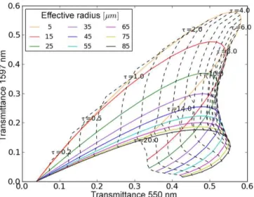
Analogous to the approach of Nakajima and King (1990), radiances at 550 and 1600 nm are stored in a lookup table as function of optical thickness and effective particle radius (Fig. 4) which can be compared to measurements. In contrast to reflectance, a wide range of this diagram shows an ambigu-ous relationship with optical thickness as transmittance first increases and then decreases with increasing optical thick-ness. The presence of an optically thin cloud increases trans-mittance by cloud particle scattering compared to the dark diffuse clear sky (Fig. 3a, solid lines). Successive increase of ice cloud optical thickness leads to increased scattering as well as to a growing degree of cloud scattering and absorp-tion. If optical thickness exceeds a critical value, cloud re-flection back to space and absorption become dominant and transmittance decreases (Fig. 3a, dashed lines).
A method has to be found to resolve the ambiguity in trans-mittance lookup tables and to separate overlapping regimes of optical thickness in Fig. 4. An important factor in distin-guishing cloud optical thickness is sky colour, which is often used for cloud detection. As optically thin clouds are partially transparent, the short-wave “blue” contribution from atmo-spheric Rayleigh scattering is visible. With increasing optical thickness the cloud scattering becomes dominant, leading to a “grey” spectrally invariant appearance. A measure for this colour is the slope of transmittance spectraTλ in the VIS
spectral range, defined as
SVIS=
100
T550 ·dTλ
dλ
λ2
λ1
. (2)
The derivative of transmittance is computed by linear re-gression in the range fromλ1=485 nm toλ2=560 nm
nor-malized by transmittance at 550 nm and scaled with 100 to obtain values in a range comparable to transmittance. Small optical thickness is associated to negativeSVIS (high
Figure 3.Ice cloud transmittance simulations at specMACS spectral sensitivity forθ0=36◦,θv=0◦,φrel=180◦and “Baum-like” habit
mixture: variation of(a)optical thickness (reff=40 µm) and(b)effective radius (τ=3.0). Thin grey vertical lines indicate 485 and 560 nm;
thick grey lines indicate 550 and 1600 nm used in the retrieval
Figure 4.Example of a lookup table of transmittance at 550 and 1600 nm simulated for θ0=36◦, θv=0◦, φrel=180◦ and habit
mixture.
fraction of blue) for larger optical thickness. The wavelength range to calculateSVISis chosen because (1) it is part of the
VIS spectrum, which is sensitive to optical thickness; (2) it exhibits a smooth spectral trend, which allows for determi-nation of a slope (cf. Fig. 3a); and (3) it is not too close to the lower end of the spectral range of specMACS where sensor sensitivity and calibration accuracy quickly deteriorate.SVIS
allows us to separate overlapping parts in Fig. 4, resulting in two widely unambiguous parts of the lookup table.
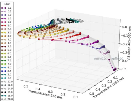
In order to exploit the information of the VIS spectral slopeSVIS, the lookup table is expanded with the slope as
a third dimension. This three-dimensional (3-D) approach is illustrated in Fig. 5. It resolves the ambiguity in conven-tional two-dimensional (2-D) lookup tables for transmittance (Fig. 4). Transmittance at 550 and 1600 nm represent the two “classical” dimensions of the lookup table.
Addition-ally, spectral slopeSVIS is used as a third. In this 3-D
dia-gram the simulated radiation values span a nonintersecting surface: points associated to larger optical thickness values are shifted to larger spectral slope values along thezaxis. Consequently, it is possible to unambiguously match a pair of optical thickness and effective radius to a measured trans-mittance spectrum in the 3-D lookup table. This approach is similar to the solutions introduced by Brückner et al. (2014) and LeBlanc et al. (2015).
3.2 Lookup table generation
The basis of the introduced retrieval method is a large set of simulated ice cloud transmittance for all required specMACS bands which are arranged in lookup tables. In this section we describe the set-up for these simulations. A standard summer midlatitude atmosphere by Anderson et al. (1986) with an ozone column scaled to 300 DU is used. The extraterrestrial solar spectrum is taken from Kurucz (1992). A horizontally homogeneous ice cloud layer is located at a base height of 9 km with a geometrical thickness of 1 km. Ice particles are assumed to be randomly orientated. The properties of this model ice cloud are varied as follows.
– 45 effective radius valuesreff ∈[5–90 µm]: increments
of 1reff=1 µm between 5 and 30 µm,1reff=2.5 µm
between 30 and 65 µm and1reff=5 µm between 65 and
90 µm;
– 60 optical thickness valuesτ ∈[0–20]: increments of
1τ=0.1 between 0 and 1.5,1τ =0.25 between 1.5 and 10 and1τ=1 between 10 and 20;
– 6 habits (solid column, hollow column, six-branch rosette, plate, droxtal, roughened aggregate) and the de-scribed habit mixture.
Solar zenith anglesθ0are simulated for the range of 24 to
Figure 5.Three-dimensional lookup table using transmittances at 550, 1600 nm and the spectral slopeSVISin the range 485–560 nm
(simu-lation forθ0=36◦,θv=0◦,φrel=180◦and habit mixture).
respect to the sun before each measurement, a very limited set of viewing zenith and azimuth angles has to be provided in the lookup table. Viewing zenith anglesθvfrom 0 to 10◦
in increments of 1◦are computed according to the sensor’s field of view during the measurements. As radiative transfer is simulated for one-dimensional horizontal homogeneous clouds, specification of relative azimuth angleφrel=φv−φ0
is sufficient. Three relative azimuth angles are taken into ac-count, because the sensor’s spatial line was either aligned parallel or perpendicular to the principal plane:φrel=0◦and
φrel=180◦(line parallel) orφrel=90◦(perpendicular).
Aerosol plays a minor role for the UFS observations evalu-ated here due to the elevevalu-ated height above the boundary layer. Nevertheless, the effect of a moderate aerosol layer on the re-trieved values was studied. Two settings are considered: one without aerosol and one assuming OPAC continental-average aerosol as provided in libRadtran (Emde et al., 2016). This aerosol mixture is based on microphysical properties of vari-ous aerosol types included in the OPAC database (Hess et al., 1998). The aerosol optical thickness was set to 0.2 at 550 nm, which is a typical value for the Meteorological Institute site in Munich. See Fig. 3 for results on specMACS spectral res-olution.
3.3 Cloud phase detection
As a first step in any ice cloud retrieval, the observed cloud thermodynamic phase has to be determined. Ice crystals and liquid droplets exhibit different absorption coefficients and consequently different cloud radiative impact. Particle ab-sorption is described by the imaginary part of the complex refractive index which depends on wavelength and phase.
For cloud-side remote sensing, Zinner et al. (2008) and Mar-tins et al. (2011) proposed to use the ratio of reflectance in narrow spectral regions at 2.1 and 2.25 µm to separate be-tween ice and liquid water. A similar approach is applied here for measurements of cloud transmittance. Ice cloud transmittance rises strongly in the wavelength range from 2.1 to 2.25 µm as absorption decreases in this spectral re-gion. In contrast, liquid water transmittance changes only slightly in the same range, corresponding to a nearly constant absorption coefficient. A NIR ratioINIR can be defined as
INIR=T2.1µm/T2.25µm, with transmittance T2.1µm at 2.1 µm
andT2.25µmat 2.25 µm. As the NIR ratio is generally smaller
for ice clouds than for water clouds, cloud phase may be de-termined by means of a threshold inINIR. We assume that
forINIR<0.92 the observed cloud consists of ice particles
and forINIR≥0.92 the observed cloud might contain liquid
water droplets. Tests using simulated data show a good per-formance of this NIR-ratio method (see Sect. 3.5), but the adequate threshold inINIRslightly depends on assumed ice
particle habit and viewing geometry. 3.4 Retrieval procedure
The algorithm to retrieve cloud optical thickness and effec-tive radius from a measurement is performed in five steps:
1. Detection of cloud phase using the NIR ratio.
2. Interpolation of an applicable lookup table from the nearest tabulated sun geometries’ values.
4. Selection of subset of close elements in lookup table.
5. Calculation of weighted average over this subset.
After detection of ice phase an applicable lookup table is obtained for the sun and sensor geometry (θv,θ0 andφrel)
given for the measurement situation. To this end, lookup ta-ble elements are interpolated from the nearest simulated ob-servation geometries’ values. For four nearest solar zenith and four nearest viewing zenith angles, the three retrieval pa-rameters (transmittance at 550, 1600 and slope 485–560 nm) are interpolated with respect to scattering angle.
In the third retrieval step, the 3-D distance δTLUT, i
be-tween one measurement and all pointsi in the interpolated lookup table is calculated as
δTLUT, i=
h
(T550−T550, i)2+(T1600−T1600, i)2+ (3)
(SVIS−SVIS, i)2
i1/2
,
with transmittance T550 at 550 nm, transmittance T1600 at
1600 nm and VIS spectral slopeSVIS, each for the measured
data as well as for pointsi=1, . . ., Nin the lookup table. The distanceδTLUT, i is directly obtained from the given values
of transmittance and transmittance slope because the overall range of values for all three measured parameters is compa-rable (compare Fig. 5).
A maximum distance accepted is set toδTmax=0.1. That
means if no points in the lookup table are found withinδTmax,
the retrieval fails. In cases for which more than three values are found, the threshold is lowered stepwise toδTmax=0.05,
0.025, 0.0125. Especially for low optical thickness, where many possible solutions lie within a small transmittance range, this improves retrieval accuracy. The distance to the closest point in the lookup tableδT is stored as a measure of retrieval significance. Significance 1−δT /δTmax=0 is
re-lated to the maximum search radius, while larger values are related to better matches and a perfect match would be sig-nificance 1. The term sigsig-nificance is chosen because the dis-tance to the tabulated values, strictly speaking, is not a mea-sure of retrieval accuracy or quality but rather a technical quantity. Given the fact that we expect matching measured and tabulated values, if we have considered the influence fac-tors correctly,δT is an important parameter which indicates the applicability of the chosen lookup table to the real mea-surement situation and consequently the reliability of the re-sults. Still this parameter could be small for the wrong rea-sons, e.g. if the impact of wrong albedo and wrong ice parti-cle habit compensate each other.
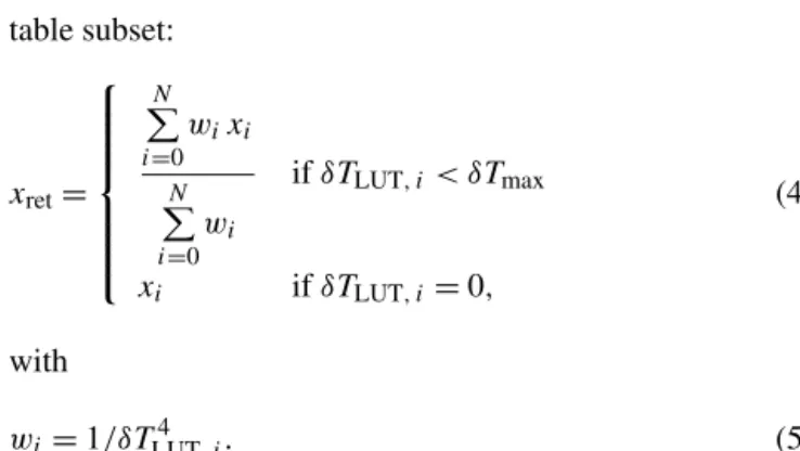
Finally, the ice cloud properties x, optical thickness and effective radius are retrieved by taking a distance weighted average over the remaining elements in the chosen lookup
table subset:
xret=
N P
i=0
wixi N
P
i=0
wi
ifδTLUT, i< δTmax
xi ifδTLUT, i=0,
(4)
with
wi=1/δTLUT, i4 . (5)
The weighting factorwis found along the following line of thought. Considering a 3-D space filled with uniformly distributed points, the number of points contributing to an averaged result increases proportional to the surface area dA=4π δT2with increasing distanceδT. To account for this factor ofδT2, the weight for each point has to be at least 1/δT2. For more emphasis on close points a smaller weight should be chosen. We usew=1/δT4.
3.5 Sensitivity tests
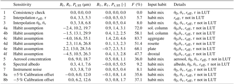
A large set of simulated cirrus transmittance spectra is used in eight retrieval test cases in order to determine typical un-certainties inherent to the presented retrieval method (and to other similar ice cloud retrievals based on transmittance or reflectance). The cloud properties retrieved from these syn-thetic cases may directly be compared to the correspond-ing simulated parameters similar to the approach in Bugliaro et al. (2011). Individual influences on retrieval accuracy can be isolated this way: test case 1 is a consistency check of whether simulated transmittance from the lookup table is lated to the correct tabulated retrieved properties by the re-trieval procedure. Using radiative transfer simulations not in-cluded in the lookup table, test cases 2 and 3 examine re-trieval sensitivity with respect to the necessary interpolation of values of the effective radius and optical thickness (case 2) and of the observation angle (case 3) in the solution space. The assumption of a fixed crystal mixture is tested against several single habit situations (case 4). Aerosol concentra-tion is varied between “no aerosol” (representative for the high-altitude measurements at UFS) and “typical aerosol” (for the area around Munich, case 5). The influence of in-accuracies in the assumed spectral surface albedo is tested (case 6). The impact of instrument noise (case 7) and cali-bration accuracy (case 8) is also evaluated applying typical values (Ewald et al., 2016). The results are summarized in Table 1.
Three error measures are provided: bias
Bx= hxret−xtruei, root mean square error (RMSE),
Rx=
p
h(xret−xtrue)2i and the 95th percentile Px,95 of
all absolute errors. xret and xtrue are retrieved and “true”
quantity (x being either τ or reff);h. . .iis the average over
Table 1. Results of sensitivity studies: retrieval bias (Br,Bτ), root mean square error (Rr, Rτ), 95 error percentile (Pr,95,Pτ,95), false
detection rateF, habit of simulated test cases and details about chosen test cases. Optical thickness of tested cases is 0.3–17 and effective radius is 8–70 (µm).
Sensitivity Br,Rr,Pr,95(µm) Bτ,Rτ,Pτ,95[-] F(%) Input habit Details
1 Consistency check 0.0, 0.0, 0.0 0.0, 0.0, 0.0 0.0 habit mix θ0,θv,reff,τin LUT
2 Interpolationreff,τ 0.4, 3.3, 5.3 −0.0, 0.5, 0.3 5.7 habit mix reff,τnot in LUT
3 Interpolationθ0,θv 0.3, 3.8, 6.8 0.0, 0.5, 0.4 8.0 habit mix θ0,θv,reff,τnot in LUT
4a Habit assumption −2.4, 10.2, 19.7 0.9, 1.4, 3.1 72.0 sol. column θ0,θv,reff,τnot in LUT
4b Habit assumption −1.5, 13.1, 29.9 0.4, 1.2, 2.5 58.1 hol. column θ0,θv,reff,τnot in LUT
4c Habit assumption −4.0, 16.6, 35.1 1.4, 2.0, 4.6 83.7 aggregate θ0,θv,reff,τnot in LUT
4d Habit assumption 2.3, 11.6, 26.8 0.1, 1.3, 2.3 51.4 rosette θ0,θv,reff,τnot in LUT
4e Habit assumption 2.2, 13.0, 28.3.6 −0.7, 2.3, 5.1 68.1 plate θ0,θv,reff,τnot in LUT
4f Habit assumption −4.5, 10.5, 26.3 0.4, 1.3, 2.8 47.7 droxtal θ0,θv,reff,τnot in LUT
5 Aerosol concentration 0.6, 9.0, 18.7 0.5, 0.8, 1.1 36.0 habit mix aerosol,θ0,θv,reff,τnot in LUT
6 Spectral albedo 0.3, 4.1, 7.6 −0.0, 0.5, 0.5 9.2 habit mix albedo,θ0,θv,reff,τnot in LUT
7 Instrument noise 0.3, 3.8, 7.0 0.0, 0.5, 0.4 8.1 habit mix θ0,θv,reff,τnot in LUT
8a +5 % Calibration offset −0.0, 6.0, 12.0 −0.1, 0.8, 1.4 35.6 habit mix θ0,θv,reff,τnot in LUT
8b −5 % Calibration offset 0.0, 6.2, 12.6 0.3, 0.8, 1.7 37.1 habit mix θ0,θv,reff,τnot in LUT
In addition, an error rateF is defined. It gives the percent-age of “incorrect” retrieval cases in the total number of per-formed retrieval tests. A test case is perceived as incorrect if the deviation of retrieved and true quantity is larger than the critical values|1reff|>5 µm and|1τ|>1 for any one of the
two quantities.
More than 30 000 tests are run for each of the following cases. Random combinations of spectra for 26 values ofτ in the range of 0.3–17, 17 values ofreff within 8–70 µm, seven
different solar zenith angles 25◦< θ0<58◦, two relative
az-imuth anglesφrel=(0◦, 180◦) and five viewing zenith angles
1◦< θ0<7◦are used.
Phase detection
The detection of ice phase worked for the vast majority of all considered test cases. Between 10 and 700 test cases out of 30 000 tests were incorrectly classified as liquid water throughout each of the 15 tests listed in Table 1, on average about 170 or 0.6 % of each case. These misclassifications are mostly related to small optical thickness around 0.5. For the ice habit tests 4a to 4f as well as 8a and 8b, up to a few 100 of 30 000 test retrievals did not succeed because no lookup table values were found near the measurement usingδTmax<0.1.
Sensitivity to interpolation in lookup table
In a first case, the retrieval is applied to spectra which are part of the lookup table for the assumed habit mixture. As an-ticipated, simulated cloud properties are exactly reproduced and all error measures assume a value of zero. For test 2 the retrieval is applied to a large set of additional synthetic ob-servations simulated for values of effective radius and cloud optical thickness that are not part of the lookup tables. In or-der to limit the number of necessary tests while not
damag-ing the validity of results, values are chosen in the followdamag-ing way: within the range covered by the variable lookup table sampling grid1x(x=τ andx=reff, values see Sect. 3.2),
random values are chosen at a distance of 0.25×1xfrom tab-ulated lookup table grid points. This is the average distance from grid points for random measurements. Each of these ice cloud test cases is simulated for 20 geometries included in the lookup tables assuming the given habit mixture. This test iso-lates the effect of interpolation of measurements within the given lookup table grid: the RMSEs are comparable to the resolution of the lookup table (in case of optical thickness) or even better (for effective radius). It is apparent that the er-ror frequency distributions are not Gaussian, but narrow dis-tributions with a few outliers. Thus, the 95th percentilePx,95
for both quantities is similar toRx. That meansRxis strongly
influenced by the outliers, while the vast majority of devia-tions are smaller. Furthermore, 5.7 % of retrieval errors are larger than the critical values|1reff|>5 µm or|1τ|>1.
In test 3, solar and viewing zenith angles used for the test observations are not part of the lookup tables either. Thus interpolation of tabulated values has to be used on other illu-mination geometries as well. Now test cases for the involved angles are chosen at locations with a distance of 0.25×1x
(withx being solar or viewing zenith angles). Azimuth an-gle is not varied, as we fix the orientation using the sun and assume that this is precise for quick measurements. Cloud parameters are varied as described for test 2.Rr andPr,95
are only slightly larger than in test 2 forreff, and hardly any
changes are detected forτ. Error rateF increases to 8 %. Sensitivity to ice crystal habit
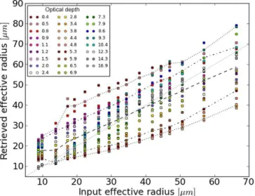
ap-Figure 6.Sensitivity to ice crystal habit (test 4d of Table 1): scatter plot for the effective radius retrieval, assuming the habit mixture. Test spectra are simulated for bullet rosettes withτ,reff,θ0andθv
not included in the lookup tables. Dashed lines indicatePr,2.5and Pr,97.5(according to 95 % of all absolute errors); dash-dotted lines
indicate±Rr; dotted lines are the means for the test cases shown:
θ0=31.75◦,θv=2.25◦,φrel=180◦.
plied to synthetic observations simulated using single habit characteristics. We apply the retrieval to the same test cases as in test 3, using lookup tables for each of the six habits (see Table 1). Compared to test 3, bias, uncertainty and er-ror rate do strongly increase due to the habit mismatch. The optical thickness retrieval is characterized by biases in the range of±1. As an example for the effective radius retrieval for one of 70 tested geometries, results for bullet rosettes are shown in Fig. 6 with coloured points indicating each of the 442 single tests and lines representing mean, standard de-viation and the interval with 95 % of all individual errors. While small effective radius values tend to be overestimated, large values are underestimated for this geometry on average. Effective radius is generally overestimated for small optical thickness below about 1. For medium optical thickness be-tween 1 and 7, the effective radius is mostly underestimated while retrievals for optical thickness larger than that have only a small bias. This behaviour can not be generalized but strongly varies with geometry and ice particle habit. The er-ror rates presented in Table 1 ranging from 48 to 84 % are probably an upper limit for the real errors, as clouds rarely consist of a single habit but rather of a habit mixture proba-bly mitigating the errors shown.
Sensitivity to aerosol and albedo situation
Besides habit assumption and interpolation techniques, aerosol optical thickness influences retrieval performance. In test 5 a retrieval assuming no aerosol is applied to the test cases of test 3, but a continental-average aerosol (Hess
et al., 1998) with an optical thickness of 0.2 at 550 nm was used to simulate the observations. The actual increase of 0.5 is larger than the aerosol mismatch, possibly caused by the fact that an even larger cloud optical thickness is needed to match larger sky brightness by aerosol due to greater forward scattering by large ice particles compared to smaller aerosol size. Not surprisingly, larger values of the RMSE and 95th percentile occur for small values ofτ, when the aerosol in-fluence on transmittance becomes predominant.
A basic assumption of the method regarding albedo is albedo influence, which is correctly represented in the lookup table, as an actual spectral albedo derived using a MODIS product over 16 days around the measurement period. Uncer-tainties still arise from the product’s uncertainty, our deriva-tion process of albedo data for the Zugspitze area and vege-tation changes during the period. As in the test case, a second albedo data set for our main measurement site in the centre of Munich is used. It is shown in light grey in Fig. 2. In the urban area, the vegetation peak between 750 and 1400 nm is much more pronounced (Munich is a “green” city), while the changes at shorter and longer wavelengths are smaller. Nonetheless, the Munich albedo data set is also brighter in the regions used for the retrieval around 550 and 1600 nm by 15 and 20 %. This increase is comparable to the difference between summer and winter for vegetated surfaces and is, at the same time, much larger than the estimate of the albedo product uncertainty (see Moody et al., 2005). Errors and un-certainties caused by such a variation of albedo are, nonethe-less, small forreff(bias at 0.3 µm, RMSE at 4 µm) andτ (no
bias, RMSE at 0.5).
Sensitivity to calibration accuracy
Another factor that influences the retrieval uncertainty is in-strument noise (cf. Sect. 2.1). In test 7, random noise is added to the synthetic observations of test 3 with a maximum mag-nitude of±0.25 % of the signal. This corresponds to a signal-to-noise ratio (SNR) of 400:1, which is a typical value found during characterization of specMACS (Ewald et al., 2016). As expected for random noise, the retrieval bias is identical to test 3, but the RMSE and false detection rate are slightly increased.
More important than the effect of instrument noise is the calibration accuracy that can be expected. A 5 % offset due to calibration is assumed for tests 8a and b, which is a con-servative estimate for specMACS for most of the covered spectrum (Ewald et al., 2016). Biases introduced are small while uncertainties, especially for effective radius, are much larger. Overall the effect is similar to the variation in aerosol content. No bias is found for the effective radius retrieval. Uncertainty values RMSE at 6 µm andPr,95 at 12 µm show
that this has to be the effect of a cancellation of opposing contributions.
sun position during the measurement. However, we expect those to be much smaller than the uncertainties discussed above. Besides, transmittance spectra are influenced by wa-ter vapour concentration in the atmosphere. For the wave-lengths used in the retrieval, which are not located close to any strong water vapour absorption bands, only small differ-ences in transmittance are to be expected. Water vapour col-umn variations between 5 and 50 kg m−2(a range as large as the difference between polar and tropical regions) only cause differences on the order of 0.1 % in transmittance.
4 Application and comparison to satellite data
In this section the presented retrieval method is applied to two cases measured during the ACRIDICON-Zugspitze campaign at the research station UFS Schneefernerhaus in October 2012. The ice cloud retrieval was applied to three specMACS data sets collected on 2 October 2012 at 08:08– 08:21, 08:57–09:10 and 09:53–10:04 UTC and two data sets collected on 3 October 2012 at 14:47–15:08 and 15:09– 15:14 UTC. Retrieval results are compared to satellite prod-ucts from Meteosat SEVIRI and MODIS. On both days SE-VIRI Rapid Scan data over the Zugspitze area were evaluated using the DLR APICS retrieval (Algorithm for the Physical Investigation of Clouds with SEVIRI; Bugliaro et al., 2011). On 2 October a TERRA overpass at 10:20 UTC almost per-fectly matched the time of the third specMACS measurement interval and comparison to MODIS collection 6 data (Plat-nick et al., 2015a) is possible. While APICS is used with a habit mixture following Baum et al. (2005), the MODIS Col-lection 6 retrieval assumes severely roughened aggregated columns (Platnick et al., 2015b).
Figure 7 shows the weather situation as seen by SEVIRI. Stationary orographic low-level cloudiness, recognisable as yellow area in the false-colour composite, is visible at the Alps (south of UFS position, red cross). On 2 October it is concentrated at the northern edge of the mountains close to the Zugspitze and east of it; on 3 October low-level cloudiness is shifted southwards. Bands of bluish synoptic-scale cirrus cloudiness not related to the lower clouds move through the area from west to east on both days. On 2 Octo-ber, the filaments of the large north–south oriented band that just passed Zugspitze were observed by specMACS a few minutes up to 2 h before the MODIS image collection time; on 3 October measurements were collected with a more ho-mogeneous cirrus deck above Zugspitze.
4.1 3 October
The later, less complex case is discussed first. For two spec-MACS data sets collected between 14:47 and 15:13 UTC on 3 October 2012 a comparison to Meteosat SEVIRI data is possible.
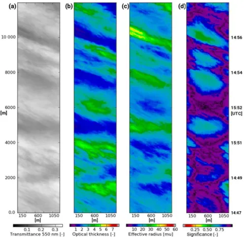
Figure 8 shows a part of the specMACS data collected on 3 October 2012 14:47–14:57 UTC. The specMACS
measure-ment was set up pointing vertically with the sensor’s spatial line of measurements perpendicular to the solar azimuth an-gle of 243◦at time of measurement (sun at south-west after local noon). Data collected by specMACS with angular res-olution of about 0.05◦(18◦field of view, 320 spatial pixels) and time resolution of 4 frames per second are regridded to approximately fill a 30 m×30 m grid using the wind speed of 18.5 m s−1(Fig. 11a) for a cloud bottom at 6500 m above UFS (cf. Fig. 7). For the case shown, the given wind direc-tion is almost aligned with the sun at south-west. That means advection was nearly perpendicular to the sensor spatial line and an almost undistorted image of the cirrus is observed by specMACS (Fig. 8). Figure 8b and c show retrievals of optical thickness and effective radius; Fig. 8d shows the re-trieval significance. Rere-trievals have been possible at rere-trieval significance values close to 0.75 and above throughout the largest part of the scene. Following our definition of this value, this means that for all pixel measurements of spec-tral transmissivity tabulated values are consistently within
δT =0.025 and 0.01 of the tabulated lookup value surface (compare Fig. 5). The real situation seems to be realistically represented by the lookup table.
It can be seen in Fig. 8b and c that optical thickness and effective radius are not totally independent. Though there could be physical reasons for this observation, it is also an inevitable effect of unknown ice crystal habit which leads to slightly varying interdependence of the used spectral chan-nels and retrieved parameters. This is inherent to all passive ice remote sensing methods based on “Nakajima–King style” retrievals.
Figure 7.Left panels: central Europe in a Meteosat false colour composite (R: 0.6 µm; G: 0.8 µm; B: inverted 10.8 µm) for 2 October 2012, 10:20 UTC (left top panel), and for 3 October 2012, 15:00 UTC (left bottom panel). Use of thermal-infrared information leads to bluish (cold, high clouds) and yellowish (warm, low clouds) colours. The red cross marks the position of UFS at Zugspitze, the black box the approximate location of MODIS data granule in Fig. 10. Right panels: related cloud radar cross sections from the vertical pointing Ka-band METEK MIRA 35 on UFS Schneefernerhaus (height 2650 m a.s.l.) around time of specMACS measurements. White areas label the time periods with ground measurements.
4.2 2 October
On one hand, the second case allows an additional compar-ison to MODIS data; on the other hand, it is complicated by low-level cloudiness which affects the satellite products. Figure 10 shows MODIS collection 6 products for 2 Octo-ber at the time of the SEVIRI measurement (10:20 UTC) as presented in Fig. 7a: effective radius, optical thickness and cloud phase. At the southern edge of the displayed do-main the low-level orographic mostly liquid water clouds can be found. Overlaid is the cirrus band moving through the area. Differences between the two cloud types are obvi-ous in optical thickness and effective radius. Water clouds are optically very thick (τ >30), while optical thickness of ice clouds ranges from 1 to 10. Effective radius retrievals for water droplets show small values (10–20 µm); ice particle re-trievals show values between 25 and 40 µm and even more than 50 µm around cloud edges. Interestingly, the above men-tioned interdependence ofτ andrreff is also visible in these
data.
The cirrus band is advected from west to east over the low water clouds with almost no change in shape and appearance (compare Meteosat and cloud radar data in Fig. 7). Thus we
analysed MODIS data over the full 2 h time period assuming a constant advection of the cloud band with wind speed. This approach is illustrated by the red lines of symbols in Fig. 10. The first symbol in the lower left corner marks the position of the specMACS sensor at UFS at the time the cloud band has just passed UFS moving east. Each symbol to west-north-west of this position is related to a time step of 133 s or about 1 km distance backward in time along wind direction. This is based on wind direction and wind speed of 8 m s−1
taken from nearby radiosonde data at cloud height of the cir-rus band from cloud radar data at the site: 4 km above UFS between 08:00 and 10:00 UTC (Fig. 7). To the left and right of the wind direction little cross symbols mark an uncertainty region as large as±1 km (MODIS pixel size) at measurement time and growing towards±8 km for a time offset of more than 2 h (related to a wind direction uncertainty of±7◦). Wa-ter cloud retrievals dominate a large part of the cross section, most likely a consequence of low water clouds forming due to topography below an optically much thinner ice cloud.
Figure 8.specMACS data at 550 nm collected above UFS on 3 October 2012, 14:47–14:57 UTC(a), retrieval of effective radius(b), optical thickness(c)and quality(d)ranging from 0 (no values in LUT within search radius) to 1 (a perfect match in the LUT). The spatial dimensions of the measurement at 2160×10 800 m are derived from cloud height (see Fig. 7) and advection wind speed.
Figure 9.Comparison of retrievals for 3 October 2012: red points show 4 s averages of specMACS retrievals for two sequences of data collection 14:47 and 15:13 UTC, and larger green dots show Meteosat SEVIRI retrievals at the position of UFS. Error bars and green shading for SEVIRI data are related to the 8-connected neighbours, and red shading for specMACS data is related to the standard deviation in all retrievals collected in a 4 s period.
(sun in the south-east before local noon,φ=142◦). As be-fore, specMACS data are regridded to onto a 30 m×30 m grid, this time with wind speed of 8 m s−1. The given wind
direction south-west means that advection was nearly paral-lel to the sensor spatial line. Thus the 2-D display of the
Figure 10.MODIS collection 6 effective radius(a), optical thickness(b)and cloud mask(c)for 2 October 2012, 10:20 UTC. Red lines of symbols are related to cross sections in time assuming advection (compare Fig. 12). The first symbol at the lower left end of these lines marks the UFS position.
Figure 11.specMACS data at 550 nm collected above UFS on 2 October 2012, 08:56–09:10 UTC(a), retrieval of effective radius(b), optical thickness(c)and retrieval significance(d)ranging from 0 (no values in LUT within search radius) to 1 (a perfect match in the LUT). The spatial dimensions of the measurement resulting 1200×5970 m are derived from cloud height (see Fig. 10) and advection wind speed.
in the scene, mostly at significance values above 0.5. Grey areas label pixels for which no tabulated values of transmit-tance were found within the maximum search radius and no retrieval is performed.
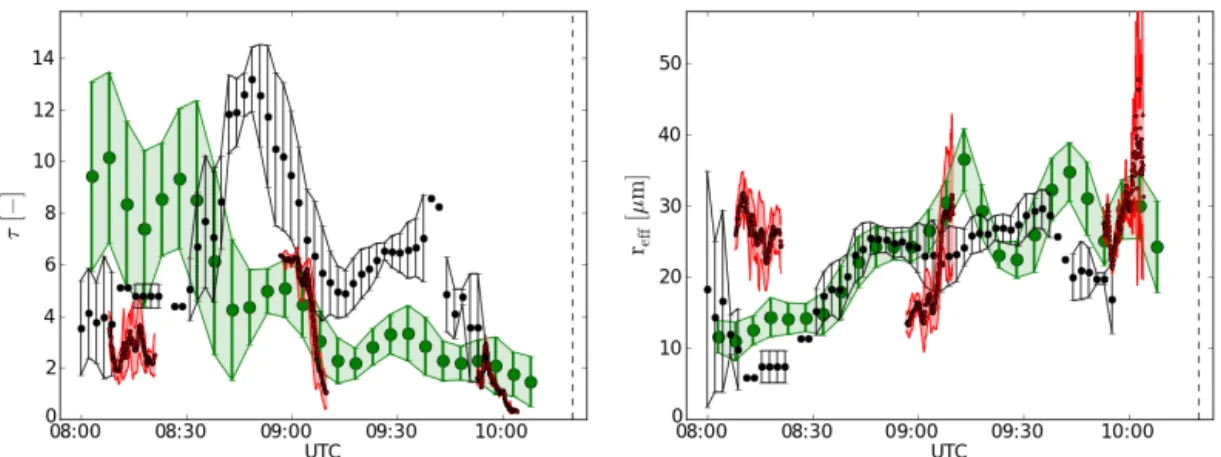
Figure 12.Comparison of retrievals for 2 October 2012: black dots show MODIS retrievals for ice clouds along the wind direction line as depicted in Fig. 10; red points show 4 s averages specMACS retrievals for three sequences of data collection (08:08–8:21, 08:57–09:10 and 09:53–10:04 UTC); larger green dots show Meteosat SEVIRI retrievals at the position of UFS. Error bars for MODIS retrievals are related to the standard deviation of retrievals in a spatial tolerance region around the wind direction (also compare to Fig. 10). The broken vertical line labels the actual time of the TERRA-MODIS overpass.
Meteosat SEVIRI retrievals. In particular, APICS detected no ice clouds after 10:05 UTC. The error bars on MODIS (black) show the standard deviation of values for all ice re-trievals in the surrounding area defined by wind direction un-certainty (Fig. 10a–c).
For optical thickness (Fig. 12a) both satellite-based re-trievals agree roughly as far as the overall value range is con-cerned. Both show a decline in optical thickness from large values around 10–13 towards small values 2–4, although they do not agree in timing of this decline. specMACS op-tical thickness agrees well with satellite retrievals around 10:00 UTC. Not surprisingly, the high-resolution transmit-tance retrieval picks up the very small values at the rear end of the cirrus band moving eastward (after 10:00) bet-ter than low-resolution reflectance retrievals from satellite. MODIS misses them completely (likely due to thick water clouds below), while SEVIRI shows larger values around 2. Given the resolution differences, specMACS retrievals are mostly within the expected uncertainty of the satellite data for 08:56–09:10 UTC (both MODIS and SEVIRI) and for 08:08–08:21 UTC (only MODIS).
For such a cirrus cloud band moving unrelated to lower-level cloudiness, optical thickness values around 10 and above – as retrieved by both satellite retrievals – are a sign of the underlying cloud layer’s influence. Chang and Li (2005) analyse these cases of thin cirrus overlaid over thicker low-level clouds in detail for MODIS data and they find simi-lar differences as seen for this scene. Water cloud and ice cloud optical thickness can not be separated from satellite perspective, while the water clouds below our observation height (UFS) obviously do not disturb the zenith observation much (compare Fig. 10d).
Effective radius values are also in good agreement for the time period 09:53–10:04 UTC. The scatter of specMACS re-trievals becomes high when optical thickness becomes very
low after 10:00 UTC. While the two satellite retrievals agree remarkably well over the whole time period, specMACS de-rived particle size is larger for the earliest measurement pe-riod 08:08–08:21 UTC. Still the observed deviation seems to be within the range of values explainable by uncertainty in-troduced through underlying water clouds with lower effec-tive radius (compare Fig. 12b).
An interesting aspect of this complex example is the demonstration of the potential of a ground-based method to provide accurate cloud properties compared to satellite meth-ods, especially for thin cirrus. The same quantities are re-trieved by both methods, utilizing similar wavelength bands, but the ground-based method benefits from its much higher spatial resolution, which allows us to separate different parts (or layers) of the observed cloudiness. In the ground-based data there might still be an impact of increased albedo (low-level cumulus below the instrument). The low (low-levels of sig-nificance of our results at larger sensor zenith angles might be a sign of it (see Fig. 12d). Nonetheless the ground-based method is less affected by this problem and generally most likely much better at retrieving thin ice cloud properties than the satellite methods.
5 Summary and discussion
We presented a new method for the retrieval of ice cloud op-tical thickness and effective radius from spectral measure-ments of transmitted radiance. Using data from a new spec-tral imager (specMACS; Ewald et al., 2016), a phase detec-tion and retrieval of optical thickness and effective radius was set up. Phase detection uses a NIR ratio of transmitted radi-ances (T2.1µm/T2.25µm). It is combined with a well known two
of transmittance retrievals with respect to increasing optical thickness. If optical thickness increases, diffusely transmitted downward radiance increases first. For increase above optical thickness of 4 to 6 radiance values decrease again. Similar to Brückner et al. (2014) and LeBlanc et al. (2015), this prob-lem is overcome by an interpretation of the spectral slope observed at 485–560 nm. This slope steadily decreases from positive values (blue sky colour) to neutral values (grey sky colour) for increasing optical thickness in this region. This slope is combined with radiances at 550 nm (mainly sensi-tive to scattering and optical thickness) and 1.6 µm to create a retrieval using a lookup table based on one-dimensional ra-diative transfer simulations.
A second important part of the presented work is the rig-orous test of sensitivities of the established retrieval to the method’s internal accuracy as well as its sensitivity to un-knowns and uncertainties of real world observations. In gen-eral, for this type of ice cloud remote sensing instrument ac-curacy (absolute calibration and noise), interpolation in the given lookup table’s forward solutions, additional scattering by unknown aerosol and unknown ice crystal habit mixture in the observed cloud have to be considered as sources of bias and uncertainty. Some of these are methodical issues. The is-sue of unknown habit is of course a core part of the physics of our objects of study. It remains an unsolved issue in the remote sensing community. The pre-calculated forward so-lutions of the retrieval have to assume a certain ice particle habit or mixture situation which most likely is not the one present for a given observation.
Using more than 300 000 synthetic measurements over the expected range of optical thickness, effective radius and ob-servation geometries, it was possible to isolate effects of these uncertainties systematically. They show that uncertain-ties due to lookup table interpolation stay minimal: system-atic deviations of optical thickness from true values are negli-gible and below 0.5 µm for effective radius. Still the variation of a specific retrieval can be in the range of 0.5 forτ and a few micrometre for effective radius. Instrument noise and un-certainty in spectral albedo create a comparably small effect. Also, unknown aerosol for moderate aerosol optical condi-tions cause systematic biases around 0.5 in τ and 0.5 µm in reff. Uncertainties of effective radius can grow to about
10 µm. The impact of limited calibration accuracy is likely to be in a similar range. Errors can be positive or negative by more than 5 µm forreffand around 1 forτ, strongly
depend-ing on the optical thickness regime. The biggest problem for retrieval accuracy is obviously unknown habit. Especially for effective radius it causes systematic errors much larger than all other influencing factors. Biases are in the order of 5 µm forreff and forτ in the order of 1. Uncertainty of a specific
retrieval can easily be wrong by more than 10 µm and 1 to 2 forτ.
Our application to two cirrus cases observed during the ACRIDICON-Zugspitze campaign in fall 2012 agreement within the expected uncertainty ranges. Given that (1)
crys-tal habit assumptions are not the same for the three com-pared methods, (2) reflectance-based methods suffer from additional uncertainty due to strong surface and cloud influ-ence from below the cirrus clouds and (3) resolution of the measurements is very different, the deviation of average opti-cal thickness values and effective radius is mostly within the observed variability in the surrounding area.
Obviously there are limitations to passive remote sensing of thin ice clouds. Chang and Li (2005) show that thin cirrus ice clouds have a long-term and large-scale average optical thickness in the range of 1 to 2 with standard deviation in the same range. In this respect the presented results seem to showcase a rather typical situation. Given these average val-ues, the possible optical thickness errors of mean values from the synthetic tests up to values of 1 and the observed dif-ferences of mean values up to 4 (though mostly much less) demonstrate the full challenge of ice cloud remote sensing.
The uncertainty values found here for the ground-based perspective are in good agreement with existing results on the satellite perspective. Key et al. (2002) anticipated differ-ences of more than 50 % in optical thickness retrievals for various habit assumptions based on simple radiative transfer considerations in the literature. In a case study for an airborne reflectance-based retrieval, Eichler et al. (2009) found rela-tive differences of around 50 % in optical thickness and up to 20 % in effective radius depending on habit assumptions. Schäfer et al. (2013) also assessed the sensitivity of their ground-based cirrus optical thickness retrieval to variation of certain parameters. The values can not be directly compared to our results, as they only refer to a small number of specific situations regarding observation geometry and cirrus situa-tion and not a large range of combinasitua-tions as in our sensi-tivity test. For variation of crystal habit and for small optical thickness up to 1 they showed large relative differences up to 80 % with average absolute differences at 0.1. Though such cases are contained in the sensitivity test shown here, aver-age impact over many different situations is smaller. Schäfer et al. (2013) also present large uncertainties for an albedo variation. This is caused by their choice of a test albedo which is extremely different from the measurement situation, while here it was assumed that the general albedo situation can be characterized well and remaining uncertainty has only small impact.
ef-fects, i.e. effects of horizontal radiation transport, are more likely to affect retrievals at higher spatial resolution.
One important technical approach is the reduction of cal-ibration inaccuracies. For example, LeBlanc et al. (2015) demonstrate retrieval approaches based on normalized radi-ance instead of absolute measurements. For their SSFR, op-erating at a similar wavelength range as specMACS (though without imaging capability), they normalize all spectral ra-diance values by the value of one spectral channel. Depen-dence on calibration accuracy is much reduced this way be-cause only the more stable channel-to-channel accuracy, has to be considered instead of absolute radiometric accuracy which is much harder to achieve. Of course the most impor-tant step forward would consist in a reduction of the crystal type uncertainty. The halo regions around 22 and 46◦ scat-tering angles were avoided here for our spectral approach. Uncertainties can be expected to be higher in these regions with strong angular gradients of transmittance under single scattering conditions, if no additional information on crystal habits is available. However, the imaging capabilities of the specMACS sensor (especially if combined with a scanning platform; see Ewald et al., 2016) do not only allow us to suc-cessfully avoid these regions for the spectral evaluation but would allow for the utilization of the spatial distribution of transmittance in these regions to provide the missing infor-mation. Use of this spatial distribution could provide impor-tant constraints regarding the present average phase function as Schäfer et al. (2013) demonstrated. Especially the pres-ence of optical scattering phenomena like type and intensity of halo displays could be used to identify specific particle shapes and orientation and information on the mixture with less perfect rough ice particles. A combination of the pre-sented method with additional information of this kind will be the next step in our effort to provide better ice cloud prop-erty observations.
6 Data availability
MODIS cloud products are available via Platnick et al. (2015a). Meteosat SEVIRI rapid scan level 1.5 radiance data can be retrieved from EUMETSAT data centre (EU-METSAT, 2016). specMACS data used in this publication and retrieval results can be found in the Supplement.
The Supplement related to this article is available online at doi:10.5194/amt-9-4615-2016-supplement.
Acknowledgements. We thank Hong Gang for providing the
single ice crystal properties from Yang et al. (2013) and three anonymous reviewers for their constructive efforts in improving this manuscript. This work was partly funded by DFG (German Research Foundation) projects MA 2548/6-1, MA 2548/9-1 and INST 86/1256-1.
Edited by: A. Kokhanovsky
Reviewed by: three anonymous referees
References
Anderson, G., Clough, S., Kneizys, F., Chetwynd, J., and Shet-tle, E.: AFGL atmospheric constituent profiles (0–120 km), Hanscom AFB, MA: Optical Physics Division, Air Force Geo-physics Laboratory,[1986]. AFGL-TR; 86-0110, US Air Force Geophysics Laboratory, Optical Physics Division, 1, 1986. Baldridge, A., Hook, S., Grove, C., and Rivera, G.: The ASTER
spectral library version 2.0, Remote Sens. Environ., 113, 711– 715, 2009.
Baran, A. J.: From the single-scattering properties of ice crystals to climate prediction: A way forward, Atmos. Res., 112, 45–69, 2012.
Barnard, J., Long, C., Kassianov, E., McFarlane, S., Comstock, J., Freer, M., and McFarquhar, G.: Development and evaluation of a simple algorithm to find cloud optical depth with emphasis on thin ice clouds, The Open Atmospheric Science Journal, 2, 46– 55, 2008.
Baum, B., Heymsfield, A., Yang, P., and Bedka, S.: Bulk scattering properties for the remote sensing of ice clouds. Part I: Micro-physical data and models, J. Appl. Meteorol., 44, 1885–1895, 2005.
Baum, B. A., Kratz, D. P., Yang, P., Ou, S. C., Hu, Y., Soulen, P. F., and Tsay, S.-C.: Remote sensing of cloud properties us-ing MODIS airborne simulator imagery durus-ing SUCCESS: 1. Data and models, J. Geophys. Res.Atmos., 105, 11767–11780, doi:10.1029/1999JD901089, 2000.
Brückner, M., Pospichal, B., Macke, A., and Wendisch, M.: A new multispectral cloud retrieval method for ship-based solar trans-missivity measurements, J. Geophys. Res., 119, 11338–11354, doi:10.1002/2014JD021775, 2014.
Bugliaro, L., Zinner, T., Keil, C., Mayer, B., Hollmann, R., Reuter, M., and Thomas, W.: Validation of cloud property retrievals with simulated satellite radiances: a case study for SEVIRI, Atmos. Chem. Phys., 11, 5603–5624, doi:10.5194/acp-11-5603-2011, 2011.
Bugliaro, L., Mannstein, H., and Kox, S.: Ice Cloud Properties From Space, in: Atmospheric Physics, edited by: Schumann, U., Re-search Topics in Aerospace, 417–432, Springer, Berlin Heidel-berg, Germany, 2012.
Buras, R., Dowling, T., and Emde, C.: New secondary-scattering correction in DISORT with increased efficiency for forward scat-tering, J. Quant. Spectrosc. Ra., 112, 2028–2034, 2011. Chang, F. L. and Li, Z.: A Near-Global Climatology of Single-Layer
and Overlapped Clouds and Their Optical Properties Retrieved from Terra/MODIS Data Using a New Algorithm, J. Climate, 18, 4752–4771, 2005.
Comstock, J., d’Entremont, R., DeSlover, D., Mace, G., Matrosov, S., McFarlane, S., Minnis, P., Mitchell, D., Sassen, K., Shupe, M., et al.: An intercomparison of microphysical retrieval algo-rithms for upper-tropospheric ice clouds, B. Am. Meteorol. Soc., 88, 191–204, 2007.
ef-fective radius: A case study, J. Geophys. Res., 114, D19203, doi:10.1029/2009JD012215, 2009.
Emde, C., Buras-Schnell, R., Kylling, A., Mayer, B., Gasteiger, J., Hamann, U., Kylling, J., Richter, B., Pause, C., Dowling, T., and Bugliaro, L.: The libRadtran software package for radia-tive transfer calculations (version 2.0.1), Geosci. Model Dev., 9, 1647–1672, doi:10.5194/gmd-9-1647-2016, 2016.
EUMETSAT: Meteosat data, available at: http://www.eumetsat. int/website/home/Data/DataDelivery/index.html, last access: 16 September 2016.
Ewald, F., Kölling, T., Baumgartner, A., Zinner, T., and Mayer, B.: Design and characterization of specMACS, a multipurpose hy-perspectral cloud and sky imager, Atmos. Meas. Tech., 9, 2015– 2042, doi:10.5194/amt-9-2015-2016, 2016.
Gasteiger, J., Emde, C., Mayer, B., Buras, R., Buehler, S., and Lemke, O.: Representative wavelengths absorption parameteri-zation applied to satellite channels and spectral bands, J. Quant. Spectrosc. Ra., 148, 99–115, doi:10.1016/j.jqsrt.2014.06.024, 2014.
Hartmann, D., Ockert-Bell, M., and Michelsen, M.: The effect of cloud type on earth’s energy balance: Global analysis, J. Climate, 5, 1281–1304, 1992.
Hausmann, P.: Ground-based remote sensing of optically thin ice clouds, 89 pp., Master’s thesis, Ludwig-Maximilians-Universität, Munich, available at: http://www.meteo.physik. uni-muenchen.de/DokuWiki/lib/exe/fetch.php?media=intern: abschlussarbeiten:2012open:ma2012_hausmann_petra.pdf (last access: 16 September 2016), 2012.
Hess, M., Koepke, P., and Schult, I.: Optical properties of aerosols and clouds: The software package OPAC, B. Am. Meteorol. Soc., 79, 831–844, 1998.
IPCC: Climate Change 2013: The Physical Science Basis. Con-tribution of Working Group I to the Fifth Assessment Report of the Intergovernmental Panel on Climate Change, edited by: Stocker, T. F., Qin, D., Plattner, G.-K., Tignor, M., Allen, S. K., Boschung, J., Nauels, A., Xia, Y., Bex, V. and Midgley, P. M., Cambridge University Press, Cambridge, UK and New York, NY, USA, 2013.
Key, J., Yang, P., Baum, B., and Nasiri, S.: Parameterization of shortwave ice cloud optical properties for various particle habits, J. Geophys. Res., 107, doi:10.1029/2001JD000742, 2002. Kurucz, R.: Synthetic infrared spectra, in: Proceedings of the 154th
Symposium of the International Astronomical Union (IAU); Tuc-son, Arizona, 2–6 March 1992, Kluwer Acad., Norwell, MA, USA, 1992.
LeBlanc, S. E., Pilewskie, P., Schmidt, K. S., and Coddington, O.: A spectral method for discriminating thermodynamic phase and re-trieving cloud optical thickness and effective radius using trans-mitted solar radiance spectra, Atmos. Meas. Tech., 8, 1361–1383, doi::10.5194/amt-8-1361-2015, 2015.
Liou, K.: Influence of cirrus clouds on weather and climate pro-cesses: A global perspective, Mon. Weather Rev., 114, 1167– 1199, 1986.
Martins, J. V., Marshak, A., Remer, L. A., Rosenfeld, D., Kauf-man, Y. J., Fernandez-Borda, R., Koren, I., Correia, A. L., Zubko, V., and Artaxo, P.: Remote sensing the vertical profile of cloud droplet effective radius, thermodynamic phase, and temperature, Atmos. Chem. Phys., 11, 9485–9501, doi:10.5194/acp-11-9485-2011, 2011.
Mayer, B. and Kylling, A.: Technical note: The libRadtran soft-ware package for radiative transfer calculations – description and examples of use, Atmos. Chem. Phys., 5, 1855–1877, doi:10.5194/acp-5-1855-2005, 2005.
McBride, P. J., Schmidt, K. S., Pilewskie, P., Kittelman, A. S., and Wolfe, D. E.: A spectral method for retrieving cloud op-tical thickness and effective radius from surface-based trans-mittance measurements, Atmos. Chem. Phys., 11, 7235–7252, doi:10.5194/acp-11-7235-2011, 2011.
McFarquhar, M., G., and Heymsfield, A. J.: The Definition and Sig-nificance of an Effective Radius for Ice Clouds, J. Atmos. Sci., 55, 2039–2052, 1998.
Moody, E. G., King, M. D., Platnick, S., Schaaf, C. B., and Gao, F.: Spatially complete global spectral surface albedos: value-added datasets derived from Terra MODIS land products, IEEE T. Geosci. Remote, 43, 144–158, doi:10.1109/TGRS.2004.838359, 2005.
Nakajima, T. and King, M.: Determination of the optical thickness and effective particle radius of clouds from reflected solar radi-ation measurements. Part I: Theory, J. Atmos. Sci., 47, 1878– 1893, 1990.
Pilewskie, P., Pommier, J., Bergstrom, R., Gore, W., Howard, S., Rabbette, M., Schmid, B., Hobbs, P., and Tsay, S.: So-lar spectral radiative forcing during the southern African regional science initiative, J. Geophys. Res., 108, 8486, doi:10.1029/2002JD002411, 2003.
Platnick, S., Ackerman, S., and King, M. E. A.: MODIS At-mosphere L2 Cloud Product (06 L2), NASA MODIS Adap-tive Processing System, Goddard Space Flight Center, USA, doi:10.5067/MODIS/MOD06_L2.006, 2015a.
Platnick, S., King, M. D., Meyer, K. G., Wind, G., Amarasinghe, N., Marchant, B., Arnold, G. T., Zhang, Z., Hubanks, P. A., Ridg-way, B., and Riedi, J.: MODIS Cloud Optical Properties: User Guide for the Collection 6 Level-2 MOD06/MYD06 Product and Associated Level-3 Datasets, MODIS documentation, available at: http://modis-atmos.gsfc.nasa.gov/MOD06_L2/atbd.html (last access: 16 September 2016), 2015b.
Sassen, K. and Comstock, J.: A midlatitude cirrus cloud climatol-ogy from the facility for atmospheric remote sensing, Part III: Radiative properties, J. Atmos. Sci., 58, 2113–2127, 2001. Sassen, K., Wang, Z., and Liu, D.: Global distribution of
cir-rus clouds from CloudSat/Cloud-Aerosol lidar and infrared pathfinder satellite observations (CALIPSO) measurements, J. Geophys. Res., 113, D00A12, doi:10.1029/2008JD009972, 2008.
Schäfer, M., Bierwirth, E., Ehrlich, A., Heyner, F., and Wendisch, M.: Retrieval of cirrus optical thickness and assessment of ice crystal shape from ground-based imaging spectrometry, At-mos. Meas. Tech., 6, 1855–1868, doi:10.5194/amt-6-1855-2013, 2013.
Stamnes, K., Tsay, S.-C., Wiscombe, W., and Jayaweera, K.: Nu-merically stable algorithm for discrete-ordinate-method radiative transfer in multiple scattering and emitting layered media, Appl. Opt., 27, 2502–2509, 1988.
Engineering Physics, Stevens Institute of Technology, Hoboken, NJ, USA, 07030, 2000.
Stephens, G. L., Tsay, S.-C., Stackhouse, Jr., P. W., and Flatau, P. J.: The Relevance of the Microphysical and Radiative Properties of Cirrus Clouds to Climate and Climatic Feedback., J. Atmos. Sci., 47, 1742–1754, 1990.
Strahler, A., Muller, J., Lucht, W., Schaaf, C., Tsang, T., Gao, F., Li, X., Lewis, P., and Barnsley, M.: MODIS BRDF/albedo prod-uct: algorithm theoretical basis document version 5.0, MODIS documentation, 1999.
Szyrmer, W., Tatarevic, A., and Kollias, P.: Ice clouds microphys-ical retrieval using 94-GHz Doppler radar observations: Basic relations within the retrieval framework, J. Geophys. Res., 117, D14203, doi:10.1029/2011JD016675, 2012.
Thomas, G. and Stamnes, K.: Radiative transfer in the atmosphere and ocean, Cambridge University Press, Cambridge, UK, 2002. Wang, C., Yang, P., Baum, B. A., Platnick, S., Heidinger, A. K.,
Hu, Y., and Holz, R. E.: Retrieval of Ice Cloud Optical Thick-ness and Effective Particle Size Using a Fast Infrared Radia-tive Transfer Model, J. Appl. Meteorol. Clim., 50, 2283–2297, doi:10.1175/JAMC-D-11-067.1, 2011.
Wang, Z. and Sassen, K.: Cirrus cloud microphysical property re-trieval using lidar and radar measurements, Part I: algorithm de-scription and comparison with in situ data, J. Appl. Meteorol., 41, 218–229, 2002.
Wendisch, M., Poeschl, U. Andreae, M., Machado, L., Albrecht, R., Schlager, H., Rosenfeld, D., Martin, S., Abdelmonem, A., Afchine, A., Araujo, A., Artaxo, P., Aufmhoff, H., Barbosa, H., Borrmann, S., Braga, R., Buchholz, B., Cecchini, M., Costa, A., Curtius, J., Dollner, M., Dorf, M., Dreiling, V., Ebert, V., Ehrlich, A., Ewald, F., Fisch, G., Fix, A., Frank, F., Fuetterer, D., Heckl, C., Heidelberg, F., Hueneke, T., Jaekel, E., Jaervinen, E., Ju-rkat, T., Kanter, S., Kaestner, U., Kenntner, M., Kesselmeier, J., Klimach, T., Knecht, M., Kohl, R., Koelling, T., Kraemer, M., Krueger, M., Krisna, T., Lavric, J., Longo, K., Mahnke, C., Manzi, A., Mayer, B., Mertes, S., Minikin, A., Molleker, S., Muench, S., Nillius, B., Pfeilsticker, K., Poehlker, C., Roiger, A., Rose, D., Rosenow, D., Sauer, D., Schnaiter, M., Schneider, J., Schulz, C., de Souza, R., Spanu, A., Stock, P., Vila, D., Voigt, C., Walser, A., Walter, D., Weigel, R., Weinzierl, B., Werner, F., Yamasoe, M. , Ziereis, H., Zinner, T. and Zoeger, M.: The ACRIDICON-CHUVA campaign:Studying tropical deep con-vective clouds and precipitation over Amazonia using the new German research aircraft HALO, B. Am. Meteorol. Soc., in press, early online release, doi:10.1175/BAMS-D-14-00255.1, 2016.
Wylie, D., Menzel, W., Woolf, H., and Strabala, K.: Four Years of Global Cirrus Cloud Statistics Using HIRS., J. Climate, 7, 1972– 1986, 1994.
Yang, P., Wei, H., Huang, H., Baum, B., Hu, Y., Kattawar, G., Mishchenko, M., and Fu, Q.: Scattering and absorption property database for nonspherical ice particles in the near-through far-infrared spectral region, Appl. Opt., 44, 5512–5523, 2005. Yang, P., Bi, L., Baum, B. A., Liou, K.-N., Kattawar, G., and
Mishchenko, M.: Spectrally consistent scattering, absorption, and polarization properties of atmospheric ice crystals at wave-lengths from 0.2 to 100 µm, J. Atmos. Sci., 70, 330–347, 2013. Zinner, T., Marshak, A., Lang, S., Martins, J. V., and Mayer, B.: