Satellite detection of multi-decadal time series of cyanobacteria accumulations in the Baltic Sea

(1)

BGD

11, 3319–3364, 2014

Cyanobacteria accumulations in the

Baltic Sea

M. Kahru and R. Elmgren

Title Page

Abstract Introduction

Conclusions References

Tables Figures

◭ ◮

Back Close

Full Screen / Esc

Printer-friendly Version Interactive Discussion

Discussion

P

a

per

|

D

iscussion

P

a

per

|

Discussion

P

a

per

|

Discuss

ion

P

a

per

|

Biogeosciences Discuss., 11, 3319–3364, 2014 www.biogeosciences-discuss.net/11/3319/2014/ doi:10.5194/bgd-11-3319-2014

Open Access

Biogeosciences

Discussions

This discussion paper is/has been under review for the journal Biogeosciences (BG). Please refer to the corresponding final paper in BG if available.

Satellite detection of multi-decadal time

series of cyanobacteria accumulations in

the Baltic Sea

M. Kahru1,2and R. Elmgren2

1

Scripps Institution of Oceanography, University of California San Diego, La Jolla, CA 92093-0218, USA

2

Department of Ecology, Environment and Plant Sciences, Stockholm University, Stockholm, Sweden

Received: 26 January 2014 – Accepted: 18 February 2014 – Published: 26 February 2014 Correspondence to: M. Kahru (mkahru@ucsd.edu)

(2)

BGD

11, 3319–3364, 2014

Baltic Sea

Title Page

Tables Figures

◭ ◮

Back Close

Full Screen / Esc

Discussion

P

a

per

|

D

iscussion

P

a

per

|

Discussion

P

a

per

|

Discuss

ion

P

a

per

|

Abstract

Cyanobacteria, primarily of the speciesNodularia spumigena, form extensive surface

accumulations in the Baltic Sea in July and August, ranging from diffuse flakes to dense

surface scum. We describe the compilation of a 35 year (1979–2013) long time series of cyanobacteria surface accumulations in the Baltic Sea using multiple satellite sensors.

5

This appears to be one of the longest satellite-based time series in biological oceanog-raphy. The satellite algorithm is based on increased remote sensing reflectance of the water in the red band, a measure of turbidity. Validation of the satellite algorithm us-ing horizontal transects from a ship of opportunity showed the strongest relationship with phycocyanin fluorescence (an indicator of cyanobacteria), followed by turbidity

10

and then by chlorophyllafluorescence. The areal fraction with cyanobacteria

accumu-lations (FCA) and the total accumulated area affected (TA) were used to characterize

the intensity and extent of the accumulations. FCA was calculated as the ratio of the number of detected accumulations to the number of cloud free sea-surface views per pixel during the season (July–August). TA was calculated by adding the area of

pix-15

els where accumulations were detected at least once during the season. FCA and

TA were correlated (R2=0.55) and both showed large interannual and decadal-scale

variations. The average FCA was significantly higher for the 2nd half of the time series (13.8 %, 1997–2013) than for the first half (8.6 %, 1979–1996). However, that does not seem to represent a long-term trend but decadal-scale oscillations. Cyanobacteria

ac-20

cumulations were common in the 1970s and early 1980s (FCA between 11–17 %), but rare (FCA below 4 %) from 1985 to 1990; they increased again from 1991 and

partic-ularly from 1999, reaching maxima in FCA (∼25 %) and TA (∼210 000 km2) in 2005

and 2008. After 2008 FCA declined to more moderate levels (6–17 %). The timing of the accumulations has become earlier in the season, at a mean rate of 0.6 days per

25

(3)

chloro-BGD

11, 3319–3364, 2014

Baltic Sea

Title Page

Tables Figures

◭ ◮

Back Close

Full Screen / Esc

Discussion

P

a

per

|

D

iscussion

P

a

per

|

Discussion

P

a

per

|

Discuss

ion

P

a

per

|

phyllain July–August sampled at the depth of∼5 m by a ship of opportunity program,

but interannual variations in FCA are more pronounced.

1 Introduction

Surface or near-surface accumulations of cyanobacteria are common in the Baltic Sea during the summer months of July and August. They are caused by massive blooms of

5

diazotrophic cyanobacteria, primarily Nodularia spumigenabut also Aphanizomenon

sp. that aggregate near the surface in calm weather (Öström, 1976; Kononen, 1992; Finni et al., 2001). Cyanobacteria blooms are considered a major environmental prob-lem in the Baltic Sea because of the loss of recreational value of the sea and the beaches due to accumulations of foul-smelling, toxic cyanobacteria, and because their

10

nitrogen fixation adds large amounts of potentially plant-available nitrogen to a eu-trophicated and largely nitrogen-limited sea (Horstmann, 1975; Larsson et al., 2001). While the general factors enhancing cyanobacteria blooms such as availability of in-organic phosphorus, high surface temperature and strong near-surface stratification are well known, the specific factors determining the magnitude and distribution of the

15

annual occurrence of these accumulations in different basins are still not understood

and quantitative assessments and models allowing prediction of the accumulations are needed. Sediment records show that cyanobacteria blooms have occurred in the Baltic Sea for thousands of years (Bianchi et al., 2000). It is often assumed that their fre-quency and intensity have increased due to anthropogenic eutrophication (Horstmann,

20

1975), but such an increase has been difficult to demonstrate at the scale of the Baltic

Sea, because of the intense patchiness and temporal variability of the blooms as well as due to the scarcity of reliable older measurements (Finni et al., 2001).

While the surface accumulations consist primarily of Nodularia spumigena, other

species of cyanobacteria, primarilyAphanizomenon sp., often dominate in the water

25

column (Hajdu et al., 2007; Rol_ffet al., 2007). These filamentous cyanobacteria have

(4)

vac-BGD

11, 3319–3364, 2014

Baltic Sea

Title Page

Tables Figures

◭ ◮

Back Close

Full Screen / Esc

Discussion

P

a

per

|

D

iscussion

P

a

per

|

Discussion

P

a

per

|

Discuss

ion

P

a

per

|

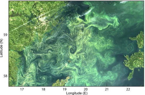
uoles are very effective backscatterers of visible light (Volten et al., 1998) and are the

major contributor to the brightness that makes the accumulations visible in satellite images (Fig. 1).

Due to their temporal and spatial variability (“patchiness”), cyanobacteria surface

accumulations are extremely difficult to monitor using ship-based sampling (Kutser,

5

2004). Their concentrations often vary by more than 2 orders of magnitude over the distance of a few meters and no suitable quantitative methods are available for reliable ground-truth measurements. Satellites sensors allow synoptic view over large spatial domains but visible and near-infrared sensors are limited to cloud-free periods. Auto-mated shipborne measurements of phycocyanin fluorescence (Seppälä et al., 2007)

10

and hyperspectral reflectance (Simis and Olsson, 2013) have the potential to provide ground-truth measurements even under cloudy conditions, but are restricted to limited horizontal transects along shipping routes. The first satellite images of the Baltic Sea

showing Nodularia accumulations were acquired by Landsat MSS in 1975 (Öström,

1976; Horstmann, 1983). However, due to the narrow swath width and low sampling

15

frequency the Landsat sensors produced only a few scenes per year for the whole

Baltic which was insu_fficient for creating quantitative time series. A problem a_ffecting

all satellite data has been the lack of quantitative algorithms for estimating cyanobac-teria concentrations as no suitable standard satellite products are available. The first quantitative satellite-based time series using the broad-band weather sensor AVHRR

20

was created in the 1990s (Kahru et al., 1994) but AVHRR data had problems separating cyanobacteria from other forms of turbidity or high surface reflectance. More sophisti-cated spectral methods that are specific to the pigment composition and other optical characteristics of cyanobacteria have been proposed (e.g. Matthews et al., 2012) but are specific to a particular set of spectral bands, e.g. those on the MERIS sensor that

25

(5)

BGD

11, 3319–3364, 2014

Baltic Sea

Title Page

Tables Figures

◭ ◮

Back Close

Full Screen / Esc

Discussion

P

a

per

|

D

iscussion

P

a

per

|

Discussion

P

a

per

|

Discuss

ion

P

a

per

|

wide-band (∼100 nm) and low signal-to-noise ratio (SNR) AVHRR sensor to modern

ocean color sensors with spectrally narrow (∼10 nm) bands and high SNR. Using these

algorithms we have compiled a quantitative time series of cyanobacteria accumulation characteristics in the Baltic Sea since 1979.

2 Data and methods

5

2.1 Satellite data

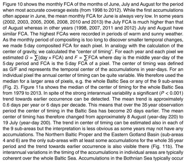
A summary of the various satellite sensors that have been used to detect cyanobac-teria from space is in Table 1. The first ocean color sensor CZCS (Hovis et al., 1980) was an experimental sensor operated by NASA from 1978 to1986 and was turned on only intermittently due to its limited recording capacity. A reasonable number of CZCS

10

scenes from the Baltic Sea are available for the July–August season from 1979 to 1984 (Table 2). CZCS data were downloaded as Level-2 files from NASA’s ocean color web (http://oceancolor.gsfc.nasa.gov/).

A broad-band weather sensor, named Advanced Very High Resolution Radiometer (AVHRR), has been flown on a series of NOAA polar orbiting satellites and data are

15

available since 1979 (Kidwell, 1995). The advantages of AVHRR are its wide swath (over 2000 km), frequent coverage (up to several passes per day), and availability over a long period of time. However, compared to specialized ocean color sensors, AVHRR has only two broadband spectral channels in the visible (0.58–0.68 µm) and near in-frared (0.72–1.10 µm) with low sensitivity and poor calibration accuracy. This makes

20

atmospheric correction difficult and limits its capability to distinguish algal blooms near

and at the surface from suspended sediments, certain types of clouds as well as bot-tom reflection in shallow areas. In spite of these limitations, AVHRR data has been used to detect bright blooms such as coccolithophores (Groom and Holligan, 1987) and cyanobacteria in the Baltic (Kahru et al., 1993, 1994, 2000; Kahru, 1997). We

25

(6)

BGD

11, 3319–3364, 2014

Baltic Sea

Title Page

Tables Figures

◭ ◮

Back Close

Full Screen / Esc

Discussion

P

a

per

|

D

iscussion

P

a

per

|

Discussion

P

a

per

|

Discuss

ion

P

a

per

|

most complete archive of AVHRR over Europe since 1979 is available from the Dundee Satellite Receiving Station (http://www.sat.dundee.ac.uk/). For detecting cyanobacteria we used only satellite passes near local noon (10:00–14:00 LT), as atmospheric scat-tering and absorption mask the relatively weak signal from the water surface at low sun elevation. While data from AVHRR sensors were transmitted daily, due to various

5

failures we have less than the maximum number of daily AVHRR datasets during the July–August period of the early years (Table 3).

Data from modern ocean color sensors are available daily with multiple passes per day and all Level-2 data files from SeaWiFS, MODIS-Aqua (MODISA), MODIS-Terra (MODIST) and VIIRS sensors of the summer months from June to August were

down-10

loaded from NASA’s ocean color archive (http://oceancolor.gsfc.nasa.gov/). The total number of files (Table 4) depends on the number and type of sensors. SeaWiFS was the only ocean color sensor operational in 1998–1999. After that period (2000 and later) data from multiple ocean color sensors were available simultaneously (Table 5). SeaWiFS Level-2 datasets are distributed in a single file whereas MODISA, MODIST

15

and VIIRS data are broken into multiple granules and therefore the number of files is higher. Between 2005 and 2010 SeaWiFS data were only available at the low (4 km) resolution (GAC) mode and were not used. We combine multiple satellite passes and multiple files per day and show the number of days in July–August with useable data (“N of valid days”) in Table 5. Scenes that were completely cloudy or produced no valid

20

data of the water surface were excluded.

All satellite data were registered to a standard equal area map in Albers conic

pro-jection with 1 km2 pixel size (Fig. 2). Since cyanobacteria blooms are not known to

occur in the Bothnian Bay, this northernmost part of the Baltic Sea was excluded from all maps and calculations. Coastal zones and other turbid areas were also excluded

25

(more below).

While we have better data coverage from 1998 and onwards (Fig. 3), even the ap-proximately 40–50 days of combined AVHRR and CZCS coverage in the early years

(7)

BGD

11, 3319–3364, 2014

Baltic Sea

Title Page

Tables Figures

◭ ◮

Back Close

Full Screen / Esc

Discussion

P

a

per

|

D

iscussion

P

a

per

|

Discussion

P

a

per

|

Discuss

ion

P

a

per

|

are relatively consistent from day to day. The detected total area approaches a plateau after about one satellite image per bloom day (Fig. 3.9 in Kahru, 1997) and the fraction of cyanobacteria accumulations (details below) are normalized to the number of clear (valid) viewings.

2.2 Methods of detecting cyanobacteria accumulations

5

2.2.1 AVHRR

The low sensitivity and poor calibration accuracy of AVHRR’s two broadband spectral

channels make accurate atmospheric correction difficult. Even with the best available

calibration coefficients, atmospheric correction often resulted in physically impossible

negative values of the water-leaving radiance (Stumpf and Fryer, 1997). We therefore

10

used the standard AVHRR band 1 albedo (Kidwell, 1995) to detect cyanobacteria. The supervised classification algorithm as applied to AVHRR data has been described pre-viously (Kahru et al., 1994; Kahru, 1997). The range of band 1 albedo of the accumula-tions was determined empirically and varied between 2.3 % and 4 %, with lower values classified as water and higher values as clouds. However, these values were used as

15

guidance and had to be empirically adjusted for some scenes. The surface distribution of cyanobacteria accumulations has a very characteristic spatial texture and patterns of swirls, eddies and filaments (Fig. 1) that are useful in separating the accumulations from clouds, fog and aircraft contrails. Areas with such high spatial texture were

con-sidered cyanobacteria accumulations. Multiple thresholdings and differences in the

vis-20

ible, near infrared and thermal channels were used to eliminate pixel areas with similar albedo. Data in the near infrared band 2 and the two thermal infrared bands, 4 (10.4– 11.0 µm) and 5 (11.6–12.2 µm), were used to screen clouds, haze, land and error pixels. Pixels with band 2 albedo values exceeding the corresponding band 1 albedo by 0.2 %

were classified as land or considered an error. Pixels with band 4 and band 5 difference

25

greater than 2◦_{C were designated as clouds. Finally, visual inspection and editing were}

(8)

BGD

11, 3319–3364, 2014

Baltic Sea

Title Page

Tables Figures

◭ ◮

Back Close

Full Screen / Esc

Discussion

P

a

per

|

D

iscussion

P

a

per

|

Discussion

P

a

per

|

Discuss

ion

P

a

per

|

and sediment-rich coastal areas. As cyanobacteria accumulations are usually present in the same location for more than one day, while clouds and other atmospheric ef-fects are more transient, sequences of images were checked for consistency of the detected accumulations over several images and suspected classification errors were manually deleted. When some of the AVHRR data were reprocessed in 2012–2013

5

to compare with modern ocean color data, some of the tests were skipped and valid ocean areas were determined as channel 1 albedo less than 4 % and the cyanobacte-ria accumulations were determined visually by their high reflectance and characteristic spatial patterns. While these methods cannot unequivocally separate isolated accumu-lations from certain thin clouds, floating pine pollen or suspended sediments in shallow

10

areas or near the coast, large-scale cyanobacteria accumulations, particularly those ofNodularia, mainly occur o_ffshore (e.g., Wasmund, 1997), away from the coast and are clearly detected. Near-shore areas with depth less than 30 m and frequent turbidity were eliminated using a fixed map (Fig. 2) as reliable separation of accumulations from other forms of turbidity was not possible in coastal areas. A sample AVHRR image

15

showing extensive cyanobacteria accumulations in band 1 albedo and the correspond-ing maps of detected accumulations as well as valid ocean area are shown in Fig. 4. A comparison of detecting the same accumulations (10 July or 11 July 2005) with the more accurate ocean color imagery (MODIS-Aqua and MODIS-Terra) is shown in Figs. 5 and 6.

20

2.2.2 Ocean color sensors

The methods applied to modern ocean color sensors such as SeaWiFS, MODISA, MODIST and VIIRS as well as the early CZCS were essentially the same as de-scribed in Kahru et al. (2007). After the 2009 reprocessing, the standard NASA ocean

color output is remote sensing reflectance (Rrs) instead of the formerly used

normal-25

ized water leaving radiance (nLw). The conversion between Rrs and nLw is

straight-forward:nLw(λ)=solar_irradiance(λ)×Rrs(λ). The semi-automated method of

(9)

BGD

11, 3319–3364, 2014

Baltic Sea

Title Page

Tables Figures

◭ ◮

Back Close

Full Screen / Esc

Discussion

P

a

per

|

D

iscussion

P

a

per

|

Discussion

P

a

per

|

Discuss

ion

P

a

per

|

(SeaWiFS) orRrs547 (MODISA and MODIST) or Rrs551 (VIIRS) and automatically

thresholdingRrsof the approximately 670 nm band (Rrs667for MODISA and MODIST,

Rrs670 for SeaWiFS, Rrs671 for VIIRS) for turbidity. High reflectance in the 670 nm band is caused by strong backscattering of particles that are either in the water column near the surface or directly at the surface (surface scum). Both near-surface and

sur-5

face backscattering is indicative of high cyanobacteria concentrations. High water re-flectance at 670 nm can also be caused by various other particles in the water column,

i.e. turbidity, such as organic and inorganic particles in river runoff or re-suspended

particles from the bottom or other particles floating at the surface (such as pine pollen). However, such other causes of turbidity or high backscattering are rare in the open

10

Baltic Sea in July and August. Thresholding of the Rrs of the red band is part of

the standard NASA level-2 processing and the Level-2 flag TURBIDW (“turbid water”)

is set ifRrs670>0.012 sr−1_{(http://oceancolor.gsfc.nasa.gov/VALIDATION/flags.html).}

For detecting cyanobacteria accumulations we also require that the flag MAXAERITER

(maximum aerosol iteration) is offas this flag is set if there is a problem in atmospheric

15

correction that often occurs near cloud edges. Using the MAXAERITER flag eliminates many false positives. A pixel is classified as a valid ocean pixel only if none of the follow-ing flags are set: ATMFAIL, LAND, HIGLINT, HILT, HISATZEN, STRAYLIGHT, CLDICE, HISOLZEN, LOWLW, CHLFAIL, MAXAERITER, ATMWARN. The primary flag here is CLDICE that indicates high reflectance due to clouds, as ice is not possible in the July–

20

August imagery. The flag COASTZ is not used. A pixel is classified as an accumulation if (1) it is a valid ocean pixel and (2) if it has the high turbidity flag set. Near-shore and

shallow areas of known high reflectance due to river runo_ffand resuspended sediments

are excluded (Fig. 2). Atmospheric correction failure sometimes occurred in the middle of the densest cyanobacteria accumulations and was caused by dense surface scum.

25

These areas in the middle of accumulations were clearly identifiable and were manually

filled with the turbid water class. They always represented a small (<5 %) fraction of the

(10)

BGD

11, 3319–3364, 2014

Baltic Sea

Title Page

Tables Figures

◭ ◮

Back Close

Full Screen / Esc

Discussion

P

a

per

|

D

iscussion

P

a

per

|

Discussion

P

a

per

|

Discuss

ion

P

a

per

|

sensitivity than MODIS data and therefore higher levels of noise variance (Hu et al., 2013). Some areas, e.g. the Gulf of Riga, are almost always turbid and the detection of cyanobacteria accumulations there is ambiguous. In these areas accumulations were confirmed only if the adjacent areas also showed accumulations.

A comparison of the results of applying the algorithms to 10–11 July 2005 imagery

5

of MODISA and MODIST (Figs. 5 and 6) shows good agreement between those two as well as AVHRR (Fig. 4).

The CZCS is less sensitive than SeaWiFS and MODIS and the TURBIDW flag is almost never set for valid ocean pixels. We therefore used the high reflectance

deter-mined asnLw555>0.8 mW cm−2_µm−1_sr−1 _{with characteristic spatial patterns to}

de-10

tect likely cyanobacteria accumulations.

2.3 Routine processing of satellite data

Multiple satellite passes (Level-2 unmapped datasets) that were classified into valid ocean and turbid classes were registered to a standard map in Albers conic equal area

projection with a 1 km2pixel size (Fig. 2) and composited into daily maps of valid ocean

15

and turbid ocean classes. Those daily maps from individual satellite sensors were then composited into merged daily maps of valid and turbid classes, respectively. For each pixel the counts of valid and turbid classes were accumulated over 5 days, one month and 2 month periods. From these counts the fraction of cyanobacteria accumulations

(FCA) was calculated as the ratio of the number of counts: N(turbid)/N(valid). FCA

20

shows the fraction of days when cyanobacteria accumulation was detected per cloud-free daily measurements. Another metric that has been used in the past, the total area (TA) or cumulative area, shows the total area where accumulations were detected at least once during the whole season (June to August). As the area of each pixel in our

standard map is 1 km2, TA in km2is equivalent to the number of detected turbid pixels in

25

the overall (seasonal) composite of turbid areas.Nodulariablooms producing surface

(11)

BGD

11, 3319–3364, 2014

Baltic Sea

Title Page

Tables Figures

◭ ◮

Back Close

Full Screen / Esc

Discussion

P

a

per

|

D

iscussion

P

a

per

|

Discussion

P

a

per

|

Discuss

ion

P

a

per

|

very low. We therefore used the July to August mean FCA as the indicator of the annual intensity of the accumulations.

A total of 1990 daily datasets (Table 5), typically merged from multiple sensors, were used over the July–August period of 1979–2013 which makes an average of over 57 days per year (out of the maximum of 62 days per July–August). The number of

indi-5

vidual scenes per day could be further increased by using the 10 year of MERIS data (2002–2011 for the July–August period) and the full-resolution SeaWiFS data for 2005– 2010. However, these data will not increase the number of daily valid datasets as these years are already well covered by other sensors.

2.4 Comparison between the outputs of different sensors

10

Satellite sensors differ in overpass times, orbits and swath widths, view and solar

an-gles, as well as spectral bands and sensitivities (e.g. signal-to-noise ratio, SNR). Their sensitivity can change over time and NASA therefore continuously monitors, and inter-mittently recalibrates and reprocesses all previously collected data. Variations between

FCA of different sensors are therefore to be expected, particularly due to differences

15

in overpass times and in the surface areas obscured by clouds. In order to evaluate the errors and variability of our FCA estimates we compared the mean monthly FCAs

obtained by multiple simultaneous sensors in 9 di_fferent areas of the Baltic Sea (Fig. 2).

Larger random variations are expected for smaller areas, e.g. the Bay of Gdansk. SeaWiFS, MODIST, MODISA and VIIRS have all overlapped temporally with at

20

least one other sensor. We used FCA obtained from MODIST (FCA_T) as the

com-mon ordinate variable in comparisons with all other sensors (Fig. 7). The results showed that FCA values obtained with temporally overlapping ocean color sensors

(SeaWiFS, MODIST, MODISA and VIIRS) were all highly correlated (R2∼0.94–0.96)

and had a linear regression with an intercept that was not significantly different from

25

zero and a slope that was close to 1.0. These conclusions were also confirmed sep-arately for individual years when FCA could be compared for two sensors. The only

(12)

ob-BGD

11, 3319–3364, 2014

Baltic Sea

Title Page

Tables Figures

◭ ◮

Back Close

Full Screen / Esc

Discussion

P

a

per

|

D

iscussion

P

a

per

|

Discussion

P

a

per

|

Discuss

ion

P

a

per

|

tained with MODISA (FCAT=1.316×FCAA+0.0015,R

2

=0.9413,N=27). The reason

for this anomaly is not clear but it is possible that the slightly higher FCAT was caused

by the higher noise level and less accurate calibration of MODIST. Another factor that

may influence the difference between sensors is the overpass time. The MODIS-Terra

overpass was at approximately 10:30 LT and the MODIS-Aqua overpass at

approxi-5

mately 13:30 LT. During calm weather it might be expected that more accumulations would develop by the afternoon, but currently we have not confirmed any systematic influence of the overpass time on FCA. FCA derived with the new VIIRS sensor corre-sponds well to FCA derived with the other sensors for the two years (2012 and 2013) available for comparison (Fig. 7c).

10

The error of the monthly FCA as determined by a satellite sensor can be estimated

as (1) the mean absolute di_fference and (2) the median absolute di_fference between

FCA values of different sensors. For MODISA, MODIST and VIIRS the mean absolute

differences were from 1.1 to 1.9 % FCA and the median absolute differences were

between 0.4 and 0.6 % FCA. For SeaWiFS the respective errors were slightly higher

15

(2.0 % and 1.1 % FCA, respectively).

Considering the highly variable nature of the accumulations and the variable orbits

covering the Baltic Sea at different times of the day, we concluded that the differences

between FCA values obtained by different ocean color sensors were insignificant and

therefore the results of individual sensors could be merged to estimate FCA.

20

Larger differences in FCA are expected when comparing the “new” ocean color

sensors with the “old” and less accurate AVHRR sensor. Due to its lower sensitivity,

AVHRR is expected to be less effective in detecting accumulations that are small or

barely above the detection limit of the more sensitive ocean color sensors. We

com-pared FCAs from the AVHRR on NOAA satellites (FCAN) with FCAs from SeaWiFS

25

(1998, 1998), MODISA (2005) and MODIST (2000, 2005) in 9 areas of the Baltic in

July and August. The overall linear regression between FCA_N and FCA has anR2 of

(13)

un-BGD

11, 3319–3364, 2014

Baltic Sea

Title Page

Tables Figures

◭ ◮

Back Close

Full Screen / Esc

Discussion

P

a

per

|

D

iscussion

P

a

per

|

Discussion

P

a

per

|

Discuss

ion

P

a

per

|

derestimation by FCA_Nis particularly evident at low FCA levels. We approximated this

relationship with a power function FCA_N₌0.95×FCA1.5 which models the lower

de-tection efficiency at low FCA and the relatively good detection efficiency at high FCA. It

appeared that the dense and large-scale accumulations were well detected by AVHRR and produced FCA values that are only slightly lower than FCAs determined

simulta-5

neously with ocean color sensors (Fig. 7d). We then used the inversion of the power

function to convert FCAN to FCA. We concluded that after applying the conversion,

FCA determined with AVHRR was comparable to FCA determined with other sensors, particularly for the intense and large-scale accumulations that mattered most in detect-ing the interannual variability.

10

2.5 Horizontal transects measured on ships of opportunity

For validating the daily images of satellite-detected cyanobacteria accumulations we used horizontal transects obtained from the Algaline (Rantajärvi, 2003) ships of

oppor-tunity instrumented with a system measuring, among others, chlorophylla(Chla)

fluo-rescence, phycocyanin (PC) fluorescence and turbidity (Seppälä et al., 2007). The

flow-15

through instrument system was installed on a ferryboat commuting between Helsinki (Finland) and Travemünde (Germany) and sampled from flow-through water pumped from approximately 5 m depth. For this analysis we used data collected during 15 tran-sects in July 2010 and provided by J. Seppälä (Finnish Environment Institute, SYKE). The measured relative voltages of PC fluorescence, Chla fluorescence and turbidity

20

were normalized between the respective minimuma and maxima and converted to a scale from 0 to 100. For each ship measurement the nearest satellite pixel was found in the corresponding daily merged image of detected accumulations and valid pixels

were averaged in the 5×5 pixel neighborhood centered at the nearest satellite pixel.

A pixel with detected accumulation was assumed to have a value of 1 and a valid pixel

25

(14)

accumula-BGD

11, 3319–3364, 2014

Baltic Sea

Title Page

Tables Figures

◭ ◮

Back Close

Full Screen / Esc

Discussion

P

a

per

|

D

iscussion

P

a

per

|

Discussion

P

a

per

|

Discuss

ion

P

a

per

|

tions during the temporal shift between satellite passes and ship measurements (up to 24 h).

3 Results

3.1 Validation of satellite detection of cyanobacteria accumulations with horizontal transects measured on ships of opportunity

5

Figure 8 shows a comparison between four ship transects of phycocyanin (PC) fluo-rescence and satellite detection of cyanobacteria accumulations on single day images in July 2010. The accumulations started to be detectable in the beginning of July in

the Bay of Gdansk (near 19◦_{E longitude) and were accurately detected by the satellite}

algorithm (Fig. 8a and b). By 10 July the accumulations were widespread both in the

10

Northern and Southern Baltic Proper (Fig. 8c and d). The narrow tongue of accumu-lations just outside of the Bay of Gdansk was well detected by both measurements.

In the southwestern Baltic the band of increased PC fluorescence (14–15◦_{E) was}

as-sociated with a few scattered detected pixels of accumulations and the corresponding average cyanobacteria score was therefore relatively low. On 12 and 20 July massive

15

accumulations covered both Northern and Southern Baltic Proper but the ship track was not optimal for detecting particularly the southern accumulations. The ship tran-sects on 12 July (west of the island of Gotland, Fig. 8e and f) and on 20 July (east of Gotland, Fig. 8g and h) were both along the edge of the major area of accumulations in the Southern Baltic Proper and that probably caused a large part of the variability in the

20

average cyanobacteria score there. Narrow strips of increased PC fluorescence corre-sponded well to detected cyanobacteria but we could not detect a common threshold of PC fluorescence above which the surface accumulations could be detected by our satellite algorithm. That was expected as the correspondence between ship measure-ments at 5 m depth and satellite measuremeasure-ments of the surface layer depends on the

25

(15)

BGD

11, 3319–3364, 2014

Baltic Sea

Title Page

Tables Figures

◭ ◮

Back Close

Full Screen / Esc

Discussion

P

a

per

|

D

iscussion

P

a

per

|

Discussion

P

a

per

|

Discuss

ion

P

a

per

|

cyanobacteria flakes (aggregates of filaments) are distributed. As our output variable

was binary (1=accumulations detected; 0=accumulations not detected), we used the

logistic regression to model the relationship between predictor variables such as PC fluorescence, Chla fluorescence or turbidity and the binary response variable. Best fits of the 2 parameters, intercept (a) and slope (b), were searched for the following

5

equation:

P = 1

1+e−(a+bX) (1)

We used the Newton–Raphson method of iteratively finding the best fit as implemented in the NMath numerical libraries (http://www.centerspace.net/). As in linear regression,

10

we were interested in finding the best model of a predictor variable to help explain the binary output. It turned out that all three predictor variables were significantly related to the detected cyanobacteria but the strongest relationship was with PC fluorescence, followed by turbidity and then by Chla fluorescence. All estimates of the goodness of fit (G-statistic, Pearson statistic, Hosmer Lemeshow statistic) showed significant

rela-15

tionships at the 0.05 level of significance. The parameters of the logistic regression were not constant from transect to transect. That was expected as the voltages were not calibrated in absolute concentrations but mostly due to the variable relationships between surface-detected accumulations and the vertical distribution of cyanobacteria in the water column (Groetsch et al., 2012). For a typical transect (15 July 2010) the

20

logistic regression parameters with PC fluorescence were: intercept 2.79 (0.05 confi-dence interval to 2.61 to 2.96), slope 0.083 (0.05 conficonfi-dence interval 0.076 to 0.090). Probability curves of the accumulations for the full ranges of predictor variables (Fig. 9) show that detected cyanobacteria accumulations were most sensitive to PC

fluores-cence and somewhat less to turbidity. The effect of Chla fluorescence had a much

25

(16)

BGD

11, 3319–3364, 2014

Baltic Sea

Title Page

Tables Figures

◭ ◮

Back Close

Full Screen / Esc

Discussion

P

a

per

|

D

iscussion

P

a

per

|

Discussion

P

a

per

|

Discuss

ion

P

a

per

|

3.2 Timing of the accumulations

Figure 10 shows the monthly FCA of the months of June, July and August for the period when most accurate coverage exists (from 1998 to 2012). While the first accumulations often appear in June, the mean monthly FCA for June is always very low. In some years (2002, 2003, 2005, 2006, 2008, 2010 and 2013) the July FCA is much higher than that

5

of August whereas in other years (1998, 2007, 2011 and 2012) July and August have similar FCA. The highest FCAs were recorded in periods of warm and sunny weather. As the monthly period of compositing is too long to discover smaller temporal changes, we made 5 day composited FCA for each pixel. In analogy with the calculation of the center of gravity, we calculated the “center of timing”. For each year and each pixel we

10

estimatedG=P(day×FCA) andF =PFCA where day is the middle year-day of the

5 day period and FCA is the 5 day FCA of a pixel. The center of timing was defined as G/F and represents the temporal center of the accumulations in year-days. For an individual pixel the annual center of timing can be quite variable. We therefore used the median for a larger area of pixels, e.g. the whole Baltic Sea or any of the 9 sub-areas

15

(Fig. 2). Figure 11a shows the median of the center of timing for the whole Baltic Sea

from 1979 to 2013. In spite of the strong interannual variability a significant (P <0.001)

trend towards earlier occurrence can be detected. The mean trend is approximately 0.6 days per year or 6 days per decade. This means that over the 35 year observation period the center of timing in the Baltic Sea has become 20 days earlier. The mean

20

center of timing has therefore changed from approximately 8 August (year-day 220) to 19 July (year-day 200). The trend in center of timing can be estimated also in each of the 9 sub-areas but the interpretation is less obvious as some years may not have any accumulations. The Northern Baltic Proper and the Eastern Gotland Basin (sub-areas 4 and 6) are the only sub-areas with at least some accumulations for the whole 35 year

25

(17)

BGD

11, 3319–3364, 2014

Baltic Sea

Title Page

Tables Figures

◭ ◮

Back Close

Full Screen / Esc

Discussion

P

a

per

|

D

iscussion

P

a

per

|

Discussion

P

a

per

|

Discuss

ion

P

a

per

|

in August, and are on average about 20 days later than in the Northern Baltic Proper (Fig. 11b). No accumulations were detected in the Bothnian Sea during 1991–1996 but they have occurred annually after that.

3.3 Time series of the mean July–August FCA

The daily datasets of the turbid and valid classes were composited into annual 2 month

5

(July–August) counts and the respective cyanobacteria fractions (FCA) were calculated (Table 5 and Fig. 12). It appears that the mean FCA of the Baltic Sea is well correlated

(R2=0.55) with the total area (TA, km2) of the accumulations. The average FCA for the

2nd half of the time series (1997–2013, 13.8 %) was significantly (P <0.01) higher than

that during the first half (1979–1996, 8.6 %) but that does not seem to represent a

sec-10

ular trend. Instead, it is suggestive of a wave-like pattern with frequent cyanobacteria

accumulations in the late 1970s and early 1980s (FCA∼5–10 %), low FCA or almost

no accumulations from 1985 to 1990, and an increase starting in 1991. Another short minimum in FCA occurred in 1995–1996. A significant increase started again in 1997. It should be noticed that the significant increase in FCA started 1 year before the start

15

of the availability of ocean color data in 1998 and that the high FCA during the years of available high-quality data is coincidental. All-time maxima in FCA and TA occurred in 2005 and 2008 and after 2008 the trend has been downward.

3.4 Spatial patterns in FCA

The spatial patterns in the annual July–August FCA (Fig. 13) show strong

year-to-20

year variability in the locations of areas with high occurrence of accumulations. For example, in 2001 and 2006 high FCA was predominantly in the south-western Baltic Sea whereas in 2007 FCA was low in the south-western Baltic and high in the north-eastern Baltic and the Gulf of Finland. These patterns can be objectively decomposed into empirical orthogonal functions (EOF) and their loadings. The dominant EOFs show

25

(18)

BGD

11, 3319–3364, 2014

Baltic Sea

Title Page

Tables Figures

◭ ◮

Back Close

Full Screen / Esc

Discussion

P

a

per

|

D

iscussion

P

a

per

|

Discussion

P

a

per

|

Discuss

ion

P

a

per

|

the total variability and has high FCA in the eastern Baltic from north to south (Fig. 14a). The second mode (EOF 2) explains 18 % of the total variability and has high FCA in the south-western Baltic (Fig. 14b). Time series of the loadings of EOFs (Fig. 14c) show years when these modes were either high or low. For example, south-western accumulations were dominant (high EOF 2) in years 2001 and 2006 and also in 2013.

5

High values of EOF 1 (years 1999, 2005 and 2008) show high FCA along the eastern side of the Baltic Sea. These years also coincide with years of overall high FCA in the Baltic Sea (Fig. 12). Low values of the respective EOF loadings show the opposite patterns. For example, years 2003 and 2011 with low EOF 2 loadings have low FCA in the south-western Baltic.

10

4 Discussion

4.1 Methods of detecting cyanobacteria accumulations

Surface accumulations of cyanobacteria are a conspicuous natural phenomenon in the Baltic Sea and are commonly observed from ships, aircraft and earth-sensing

satel-lites. The earliest report of a surface accumulation identified asNodulariain the Baltic

15

seems to be from the summer of 1901 observed from a ship in the southern Baltic

(Ap-stein, 1902), i.e. over 110 years ago. The first scientific satellite observation of a

Nodu-lariaaccumulation was made in 1973 (Öström, 1976), possibly the very first applica-tion of satellite technology in biological oceanography. While anecdotal observaapplica-tions of cyanobacteria accumulations in the Baltic are common, quantitative time series are

20

difficult to obtain. For example, the sampling frequencies of official oceanographic

mon-itoring programs are typically too coarse in space and time to create reliable time series (e.g. Finni et al., 2001). Satellite sensors often provide visually stunning imagery but quantitative time series are hard to compile. Moreover, time series generated from one satellite sensor are not necessarily compatible with time series generated from another

25

(19)

quanti-BGD

11, 3319–3364, 2014

Baltic Sea

Title Page

Tables Figures

◭ ◮

Back Close

Full Screen / Esc

Discussion

P

a

per

|

D

iscussion

P

a

per

|

Discussion

P

a

per

|

Discuss

ion

P

a

per

|

tative interannual time series of sufficient length. In the era of anthropogenic climate

change it is common and justified to look for trends in environmental variables but the observed changes in relatively short time series are most often due to decadal or in-terannual variability rather than to secular trends. In order to build time series that are as long as possible, we used multiple satellite sensors and included both the “old” and

5

“new” datasets.

Several algorithms using spectral bands in the red and the “red edge” portion of the near-infrared spectrum can be applied to MERIS data for the detection of cyanobacte-ria, e.g. the fluorescent line height (FLH, Gower et al., 1999), the maximum chlorophyll index (MCI, Gower et al., 2006), the cyanobacteria index (CI, Wynne et al., 2008) and

10

the Maximum Peak Height (MPH, Matthews et al., 2012). Hyperspectral sensors, e.g. HICO (Lucke et al., 2011), have even more potential in creating algorithms that are specific to particular features in the absorption, fluorescence or backscattering spectra of cyanobacteria. While these algorithms are potentially more accurate for separating cyanobacteria from other types of algae and other substances in the water, they are

15

specific to the band sets of particular sensors (e.g. MERIS). Therefore those algorithms cannot be extended backwards to the early sensors. We therefore did not attempt to use these spectral methods of detecting cyanobacteria. An important factor in the ap-plication of these spectral algorithms is that the optical characteristics of cyanobacteria accumulations are very sensitive to their vertical distribution. As water absorbs strongly

20

in the red part of the spectrum, it makes a drastic difference to the reflectance

spec-trum if the accumulations extend slightly above the water surface (i.e. surface scum) or are submerged just under the air–water interface. A sudden increase in wind speed can quickly change the vertical structure of the accumulations, mix the accumulations in the upper few meters and drastically change the output of algorithms that are too

25

(20)

BGD

11, 3319–3364, 2014

Baltic Sea

Title Page

Tables Figures

◭ ◮

Back Close

Full Screen / Esc

Discussion

P

a

per

|

D

iscussion

P

a

per

|

Discussion

P

a

per

|

Discuss

ion

P

a

per

|

hyper-spectral algorithms are not applicable to old sensors like AVHRR with only one band in the visible part of the spectrum. In order to create a series as long as possible

using different kinds of satellite sensors including those with low signal-to-noise ratio,

we opted to use simple, generic algorithms that are sensitive to brightness in the red part of the spectrum.

5

It is technically challenging to create a consistent time series that combines data from multiple satellite sensors over a long time period. We have here provided meth-ods for linking estimates of FCA from the “old” AVHRR and CZCS sensors with those from the “new” ocean color sensors, and created a 35 year long time series of the fre-quency of cyanobacteria accumulations in the Baltic Sea. While our satellite data are

10

limited to cloud-free periods and detect the presence cyanobacteria only by their sur-face signature, the relative temporal consistency of the accumulations and the large number of satellite measurements (Table 4) gives us confidence in the interannual time

series. It is difficult to compare our interannual time series with the results from the

traditional monitoring programs which typically sample a few fixed stations once per

15

month. A single monthly sample can easily miss the high cyanobacteria concentration in a plume floating nearby (e.g. Finni et al., 2001) and the mean error for the more

stable chlorophyll a concentration has been estimated to be ∼100 % due to

tempo-ral aliasing and another∼100 % due spatial heterogeneity (Kahru and Aitsam, 1985).

Higher temporal and spatial frequency is provided by programs like Algaline

(Ranta-20

järvi, 2003) using ships of opportunity. However, the Chla in vivo fluorescence that is often used as a measure of phytoplankton biomass is a poor measure of the abundance of cyanobacteria as most of the cyanobacterial Chla is located in the non-fluorescing photosystem I (Seppälä et al., 2007 and references therein). It was also confirmed in this work that Chla florescence was a worse predictor for detecting cyanobacteria

25

(21)

BGD

11, 3319–3364, 2014

Baltic Sea

Title Page

Tables Figures

◭ ◮

Back Close

Full Screen / Esc

Discussion

P

a

per

|

D

iscussion

P

a

per

|

Discussion

P

a

per

|

Discuss

ion

P

a

per

|

Preliminary comparison between Chla values extracted from discrete water samples provided by S. Kaitala (Finnish Environment Institute, SYKE) and FCA along the ship tracks where samples were collected showed quite similar interannual patterns. The

mean chlorophylla concentration of samples collected in July–August in the Eastern

Gotland basin had a coherent pattern with FCA (R=0.69, Fig. 15) but much lower

5

variability (mean=3.8 mg m−3_{, coe}

fficient of variation=0.22). The corresponding time

series of FCA had a coefficient of variation that was 4–5 times higher (1.03 for 1995–

2012 and 1.34 for 1979–2013). This difference in variability was expected as Chla

integrates all phytoplankton whereas FCA is a much more sensitive parameter as the detection of surface accumulations requires very high concentrations of

cyanobacte-10

ria (primarilyNodularia) near the surface. An analysis of the environmental conditions

explaining the interannual patterns in FCA (cf. Kahru et al., 2007) is planned for the fu-ture. Future work should also compare this FCA dataset with the more advanced multi-and hyperspectral methods like the Maximum Peak Height (Matthews et al., 2012).

Acknowledgements. Financial support was provided to R. E. by the Swedish Research

Coun-15

cil Formas and the Stockholm University’s Baltic Ecosystem Adaptive Management Program. Satellite ocean color data were provided by the NASA Ocean Color Processing Group. AVHRR data were provided by Dundee Satellite Receiving Station. The authors thank S. Kaitala for

providing Algaline extracted chlorophylladata, J. Seppälä for providing the Algaline transect

data, T. Tamminen and Oleg Savchuk for useful discussions and Andrew Brooks for AVHRR

20

data conversion.

References

Apstein, C.: Das Plankton der Ostsee (Holsatia Expedition 1901), Abhandl. Deutschen Seefischerei-Vereins, VII, 103–129, 1902 (In German).

Bianchi, T. S., Engelhaupt, E., Westman, P., Andren, T., Rolff, C., and Elmgren, R.:

Cyanobac-25

(22)

BGD

11, 3319–3364, 2014

Baltic Sea

Title Page

Tables Figures

◭ ◮

Back Close

Full Screen / Esc

Discussion

P

a

per

|

D

iscussion

P

a

per

|

Discussion

P

a

per

|

Discuss

ion

P

a

per

|

Finni, T., Kononen, K., Olsonen, R., and Wallström, K.: The history of cyanobacterial blooms in the Baltic Sea, Ambio, 30, 172–178, 2001.

Gower, J., Hu, C., Borstad, G., and King, S.: Ocean color satellites show extensive lines of

floatingSargassumin the Gulf of Mexico, IEEE T. Geosci. Remote, 44, 3619–3625, 2006.

Gower, J. F. R., Doerffer, R., and Borstad, G.: Interpretation of the 685 nm peak in water-leaving

5

radiance spectra in terms of fluorescence, absorption and scattering, and its observation by MERIS, Int. J. Remote Sens., 20, 1771–1786, 1999.

Hajdu, S., Höglander, H., and Larsson, U.: Phytoplankton vertical distributions and composition in Baltic Sea cyanobacterial blooms, Harmful Algae, 6, 187–205, 2007.

Horstmann, U.: Eutrophication and mass occurrence of blue-green algae in the Baltic,

Meren-10

tutkimuslait, Julk/Havsforskningsinst Skr., 239, 83–90, 1975.

Horstmann, U.: Distribution patterns of temperature and water colour in the Baltic Sea as recorded in satellite images: indicators of plankton growth, Berichte Institut für Meereskunde Universität Kiel, 106, 1–147, 1983.

Hovis, W. A., Clark, D. K., Anderson, F., Austin, R. W., Wilson, W. H., Baker, E. T., Ball, D.,

15

Gordon, H. R., Mueller, J. L., El-Sayed, S., Sturm, B., Wrigley, R. C., and Yentsch, C. S.: NIMBUS-7 Coastal Zone Color Scanner: System description and initial imagery, Science, 210, 60–63, 1980.

Hu, C., Feng, L., and Lee, Z.: Uncertainties of SeaWiFS and MODIS remote sensing re-flectance: implications from clear water measurements, Remote Sens. Environ., 133, 168–

20

182, 2013.

Groom, S. B. and Holligan, P. M.: Remote sensing of coccolithophore blooms, Adv. Space Res., 7, 73–78, 1987.

Kahru, M. and Aitsam, A.: Chlorophyll variability in the Baltic Sea: a pitfall for monitoring, J. Cons. Int. Explor. Mer., 42, 111–115, 1985.

25

Kahru, M., Leppänen, J.-M., and Rud, O.: Cyanobacterial blooms cause heating of the sea surface, Mar. Ecol.-Prog. Ser., 101, 1–7, 1993.

Kahru, M., Horstmann, U., and Rud, O.: Satellite detection of increased cyanobacteria blooms in the Baltic Sea: natural fluctuation or ecosystem change?, Ambio, 23, 469–472, 1994. Kahru, M.: Using satellites to monitor large-scale environmental change: a case study of

30

(23)

BGD

11, 3319–3364, 2014

Baltic Sea

Title Page

Tables Figures

◭ ◮

Back Close

Full Screen / Esc

Discussion

P

a

per

|

D

iscussion

P

a

per

|

Discussion

P

a

per

|

Discuss

ion

P

a

per

|

Kahru, M., Leppänen, J.-M., Rud, O., and Savchuk, O. P.: Cyanobacteria blooms in the Gulf of Finland triggered by saltwater inflow into the Baltic Sea, Mar. Ecol.-Prog. Ser., 207, 13–18, 2000.

Kahru, M., Savchuk, O. P., and Elmgren, R.: Satellite measurements of cyanobacterial bloom frequency in the Baltic Sea: interannual and spatial variability, Mar. Ecol.-Prog. Ser., 343,

5

15–23, doi:10.3354/meps06943, 2007.

Kidwell, K. B.: NOAA Polar Orbiter Data Users Guide (TIROS-N, 6, 7, NOAA-8, NOAA-9, NOAA-10, NOAA-11, NOAA-12, NOAA-14), National Oceanic & Atmospheric Administration, Washington DC, 1995.

Kononen, K.: Dynamics of the toxic cyanobacterial blooms in the Baltic Sea, Finnish Mar. Res.,

10

261, 3–36, 1992.

Kutser, T.: Quantitative detection of chlorophyll in cyanobacterial blooms by satellite remote sensing, Limnol. Oceanogr., 49, 2179–2189, 2004.

Larsson, U., Hajdu, S., Walve, J., and Elmgren, R.: Estimating Baltic nitrogen fixation from the summer increase in upper mixed layer total nitrogen, Limnol. Oceanogr., 46, 811–820, 2001.

15

Lucke, R. L., Corson, M., McGlothlin, N. R., Butcher, S. D., Wood, D. L., Korwan, D. R., Li, R. R., Snyder, W. A., Davis, C. O., and Chen, D. T.: Hyperspectral Imager for the Coastal Ocean: instrument description and first images, Appl. Optics, 50, 11, 1501–1516. 2011.

Matthews, M. W., Bernard, S., and Robertson, L.: An algorithm for detecting trophic status

(chlorophylla), cyanobacterial-dominance, surface scums and floating vegetation in inland

20

and coastal waters, Remote Sens. Environ., 124, 637–652, 2012.

Öström, B.: Fertilization of the Baltic by nitrogen-fixation in the blue-green alga Nodularia

spumigena, Remote Sens. Environ., 4, 305–310, 1976.

Rantajärvi, E.: Alg@line in 2003, 10 years of innovative plankton monitoring and research and operational information service in the Baltic Sea, Meri – Report Series of the Finnish Institute

25

of Marine Research, 48, 58 pp., 2003.

Rolff, C., Almesjö, L., and Elmgren, R.: Nitrogen fixation and the abundance of the diazotrophic

cyanobacteriumAphanizomenon sp. in the Baltic Proper. Mar. Ecol.-Prog. Ser., 332, 107–

118, 2007.

Seppälä, J., Ylöstalo, P., Kaitala, S., Hällfors, S., Raateoja, M., and Maunula, P.:

Ship-of-30

(24)

BGD

11, 3319–3364, 2014

Baltic Sea

Title Page

Tables Figures

◭ ◮

Back Close

Full Screen / Esc

Discussion

P

a

per

|

D

iscussion

P

a

per

|

Discussion

P

a

per

|

Discuss

ion

P

a

per

|

Simis, S. G. H. and Olsson, J.: Unattended processing of shipborne hyperspectral reflectance measurements, Remote Sens. Environ., 135, 202–212, 2013.

Simis, S. G. H., Peters, S. W. M., and Gons, H. J.: Remote sensing of the cyanobacterial pigment phycocyanin in turbid inland water, Limnol. Oceanogr., 50, 237–245, 2005.

Stumpf, R. P. and Frayer, M. L.: Use of AVHRR imagery to examine long-term trends in water

5

clarity in coastal estuaries: example in Florida Bay, in: Monitoring Algal Blooms: New Tech-niques for Detecting Large-Scale Environmental Change, edited by: Kahru, M. and Brown, C. W., Springer Verlag Berlin, Heidelberg, New York, 1–24, 1997.

Volten, A. H., Haan, J. F. D., Hovenier, J. W., Schreurs, R., Vassen, W., Dekker, A. G., Hoogen-boom, J., Charlton, F., and Wouts, R.: Laboratory Measurements of Angular Distributions of

10

Light Scattered by Phytoplankton and Silt, Limnol. Oceanogr., 43, 1180–1197, 1998. Walsby, A. E.: Gas vesicles, Microbiol. Rev., 58, 94–144, 1994.

Wasmund, N.: Occurrence of cyanobacterial blooms in the Baltic Sea in relation to environmen-tal conditions, Int. Revue Gesamten Hydrobiol., 82, 169–184, 1997.

Wynne, T. T., Stumpf, R. P., Tomlinson, M. C., Warner, R. A., Tester, P. A., Dyble, J., and

Fah-15

(25)

BGD

11, 3319–3364, 2014

Baltic Sea

Title Page

Tables Figures

◭ ◮

Back Close

Full Screen / Esc

Discussion

P

a

per

|

D

iscussion

P

a

per

|

Discussion

P

a

per

|

Discuss

ion

P

a

per

|

Table 1.Characteristics of satellite sensors used to detect cyanobacteria accumulations in the Baltic Sea.

Sensor Satellite Agency Spatial Temporal Signal to noise

resolution, m resolution, days ratio of the red band

MSS Landsat 2 NASA/USGS 83 18 40

TM Landsat 5 NASA/USGS 30 16 50

CZCS Nimbus-7 NASA 825 irregular 110

AVHRR NOAA-X NOAA 1100 <1 3

SeaWiFS Orbview-2 NASA 1100 ∼2 390

MODIS Terra NASA 250/500/1000 ∼2 1000

MODIS Aqua NASA 250/500/1000 ∼2 1000

MERIS ENVISAT ESA 300/1200 ∼3 883

(26)

BGD

11, 3319–3364, 2014

Baltic Sea

Title Page

Tables Figures

◭ ◮

Back Close

Full Screen / Esc

Discussion

P

a

per

|

D

iscussion

P

a

per

|

Discussion

P

a

per

|

Discuss

ion

P

a

per

|

Table 2.Number of CZCS scenes over the Baltic Sea available for Juyl–August.

1979 1980 1981 1982 1983 1984 1985

(27)

BGD

11, 3319–3364, 2014

Baltic Sea

Title Page

Tables Figures

◭ ◮

Back Close

Full Screen / Esc

Discussion

P

a

per

|

D

iscussion

P

a

per

|

Discussion

P

a

per

|

Discuss

ion

P

a

per

|

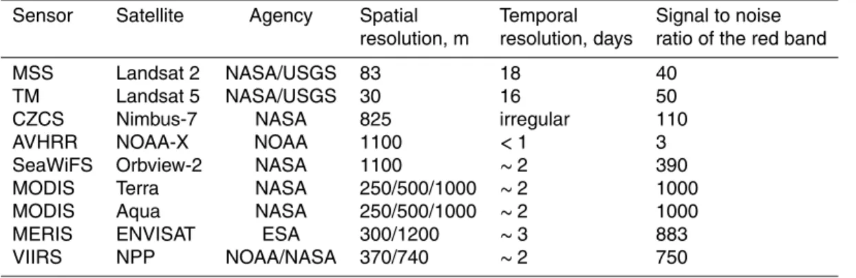
Table 3.Number of AVHRR scenes over the Baltic Sea available for July–August.

1979 1980 1981 1982 1983 1984 1985

33 40 32 37 39 34 46

1986 1987 1988 1989 1990 1991 1992

47 66 68 59 61 62 64

1993 1994 1995 1996 1997 1998 1999

(28)

BGD

11, 3319–3364, 2014

Baltic Sea

Title Page

Tables Figures

◭ ◮

Back Close

Full Screen / Esc

Discussion

P

a

per

|

D

iscussion

P

a

per

|

Discussion

P

a

per

|

Discuss

ion

P

a

per

|

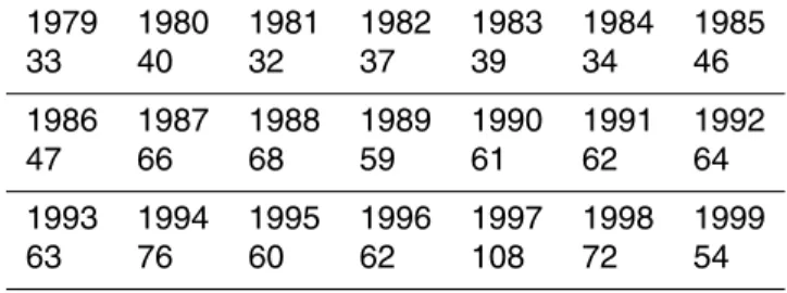
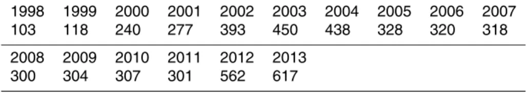
Table 4. Number of combined scenes of SeaWiFS, MODIST, MODISA and VIIRS over the Baltic Sea available for July–August.

1998 1999 2000 2001 2002 2003 2004 2005 2006 2007

103 118 240 277 393 450 438 328 320 318

2008 2009 2010 2011 2012 2013

(29)

BGD

11, 3319–3364, 2014

Baltic Sea

Title Page

Tables Figures

◭ ◮

Back Close

Full Screen / Esc

Discussion

P

a

per

|

D

iscussion

P

a

per

|

Discussion

P

a

per

|

Discuss

ion

P

a

per

|

Table 5.Number and type of daily detected (“turbid”) and useable (“valid”) satellite datasets, mean fraction of cyanobacteria accumulations (FCA%), total area covered by accumulations (TA) over the Baltic Sea and the sensors used in the analysis.

Year Nof turbid days Nof valid days FCA% TA, 1000 km2 Sensor

1979 17 40 11.2 57 CZCS, AVHRR

1980 23 54 11.7 59 CZCS, AVHRR

1981 17 39 16.8 91 CZCS, AVHRR

1982 21 42 12.9 69 CZCS, AVHRR

1983 27 47 12.3 78 CZCS, AVHRR

1984 13 39 17.0 86 CZCS, AVHRR

1985 9 41 1.1 3 AVHRR

1986 11 47 3.3 14 AVHRR

1987 2 61 0.4 1 AVHRR

1988 7 61 2.1 8 AVHRR

1989 16 56 3.9 23 AVHRR

1990 16 61 3.8 26 AVHRR

1991 19 60 10.2 74 AVHRR

1992 20 60 13.1 60 AVHRR

1993 14 61 6.9 39 AVHRR

1994 21 46 14.3 103 AVHRR

1995 24 60 4.3 40 AVHRR

1996 22 61 2.3 21 AVHRR

1997 35 62 16.0 127 AVHRR

1998 48 62 5.9 129 SeaWiFS, AVHRR

1999 55 62 21.6 209 SeaWiFS, AVHRR 2000 59 62 13.1 178 SeaWiFS, MODIST 2001 55 62 12.4 139 SeaWiFS, MODIST 2002 59 62 14.5 176 SeaWiFS, MODISA, MODIST 2003 59 62 17.9 176 SeaWiFS, MODISA, MODIST 2004 59 62 9.5 155 SeaWiFS, MODISA, MODIST 2005 58 62 25.0 183 MODISA, MODIST 2006 60 62 14.8 174 MODISA, MODIST

2007 56 62 7.1 110 MODISA, MODIST

2008 57 62 25.5 212 MODISA, MODIST

2009 54 62 6.1 160 MODISA, MODIST

2010 55 62 10.7 143 MODISA, MODIST 2011 61 62 16.5 186 MODISA, MODIST 2012 61 62 9.1 155 MODISA, MODIST, VIIRS 2013 62 62 11.1 165 MODISA, MODIST, VIIRS 1979– Total Total Mean Mean

(30)

BGD

11, 3319–3364, 2014

Baltic Sea

Title Page

Tables Figures

◭ ◮

Back Close

Full Screen / Esc

Discussion

P

a

per

|

D

iscussion

P

a

per

|

Discussion

P

a

per

|

Discuss

ion

P

a

per

|

59

58

17 18 19 20 21 22

Longitude (E)

Latitude (N)

(31)

BGD

11, 3319–3364, 2014

Baltic Sea

Title Page

Tables Figures

◭ ◮

Back Close

Full Screen / Esc

Discussion

P

a

per

|

D

iscussion

P

a

per

|

Discussion

P

a

per

|

Discuss

ion

P

a

per

|

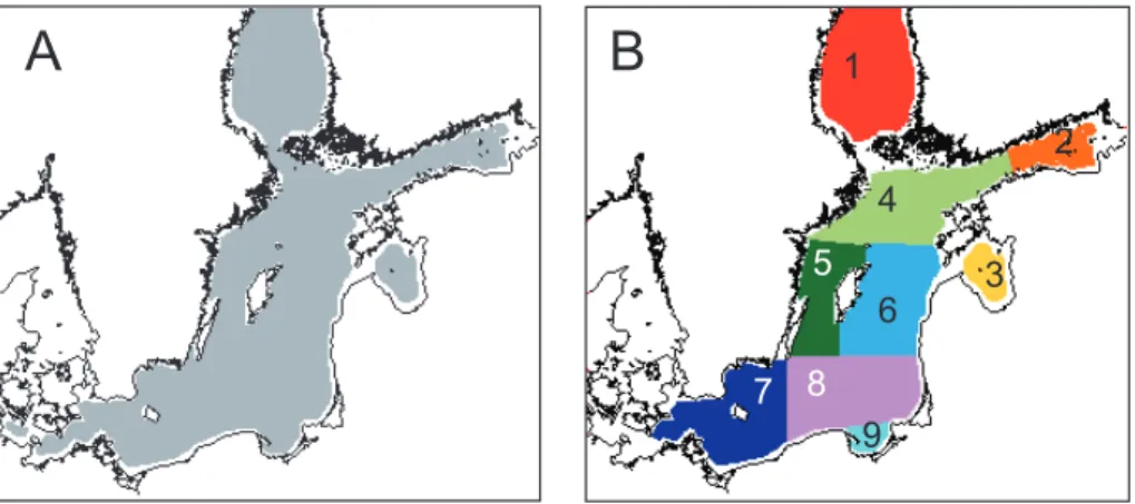
Fig. 2.Study areas in the Baltic Sea.(A)The area considered (grey) in mapping cyanobacteria blooms excludes near-shore areas with potentially high turbidity (white, 19.5 % of the total sea

area).(B)Partition into nine 9 separate basins: Bothnian Sea (BS, 1), Gulf of Finland (GF, 2),