Gilberto Fisch
Instituto de Aeronáutica e Espaço (IAE) São José dos Campos – Brazil
Comparisons between aerovane
and sonic anemometer wind
measurements at Alcântara
Launch Center
Abstract: This paper aimed to compare the wind measurements in two different types of anemometer: classical aerovane and modern sonic anemometer. The two sensors were installed at Alcântara Launch Center during a dry period of 2008 at 10 m height. The analysis compared the average and maximum wind speed for one- and ten-minute time intervals for each anemometer. The results showed that, considering the range of the measurements (from 3.0 up to 6.5 m/s), the average and maximum wind speed are different by roughly 0.5 and 1.0 m/s, respectively. There is no signiicant difference between the results from one- and ten-minute time intervals. The substitution of the sensors at the Anemometric Tower at Alcântara Launch Center will lead to an increase of the average and maximum wind speed.
Keywords: Masts, Wind speed, Maximum wind.
INTRODUCTION
The Alcântara Launch Center (ALC) is the place from where the Brazilian space vehicles (sounding rockets and the Satellite Launcher Vehicle) are launched. The knowledge of the vertical proile of the wind (in terms of direction and wind speed) and its association with the meteorological systems are very important, especially for the improvement of safety in the activities related to the preparation, integration and launching of rockets (Johnson, 2008). According to Altino and Barbré (2009), the mostly requested information about the environment in the US Space Facility is related with the winds.
The winds can be split in upper air (from 200 m up to 30 km and usually made with radiosondes) and surface winds (from the surface up to 200 m). This latter layer is known as the Atmospheric Surface Layer (ASL) and it is the region at the bottom of the atmosphere where turbulent fluxes are almost constant (varies less than 10% of their magnitude). The turbulence is continuously being generated and/or dissipated, and this layer also suffers the diurnal cycle of solar heating (Fisch, 2009).
Recently, Gisler (2009) carried out a detailed statistical study about the wind characteristics at ASC using the aerovane wind sensors. These sensors have been mounted in a wind tower named Anemometric Tower (70 m height), and it is collecting data at Alcântara
Launch Center since 1995. These measurements have been used to determine the wind climatology (Pereira, 2002; Gisler, 2009), the wind proile and turbulence characteristics (Fisch, 1999; Roballo and Fisch, 2008), as well as to determine the rocket trajectory during launching missions (Leão, 2009). However, with the technology development of the sensors, the ASC authorities are concerned with substituting the old technology from the aerovanes for modern instruments that use the sonic technique. The Space Kennedy Center (KSC) is also suffering a modernization process of these sensors (Short and Wheeler, 2006) as well as others public and private organizations in US (for instance Wastrack et al., 2000). Speciically, the KSC had collected data during 18 days (from 13 up to 30 May 2005) at Cape Canaveral (Florida) at ive different towers nearby (their heights ranged from 3 up to 145 m). The one-minute observation from sonic and aerovanes were measured at parallel booms at the same height (see details at Short and Wheeler, 2006). When these instrumentation’s modiication would inish, attention should be given to preservation of the time series of the substituted anemometers (compatibility between the old and new time series) as well as to adapting the space launching procedures of using the new sensors (the rules used by Safety Flight Group).
This study aims to compare two different sensors (aerovane and sonic anemometer) by analyzing the difference in average wind speed and maximum wind speed. The data has been collected in a ield campaigns held at ALC. This study also aims to contribute to the knowledge of the time series analysis of wind data at Alcântara Launch
Center in order to preserve the homogeneity of the data for climatology purposes.
DATA, SITE AND METHODS
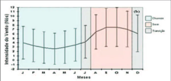
The climatic pattern at Alcântara shows two distinct rainfall regimes: a dry and a wet season. The Figure 1 shows the rainfall climatic pattern. The dry season is from August to November and it is characterized by strong winds (the average wind is 7.0 m/s) due to the intensiication of the thermal contrast between the continent and adjacent ocean (Fisch, 1999). This will trigger a sea breeze circulation which is superimposed to the trade winds producing these strong winds. The wet season is from January to June, being the months of March and April the rainiest ones (Guedes and Oyama, 2004). The data-set used in this work has been collected during an intensive ield campaign (named Operação Murici II) held at ASC from 19 to 25 September 2008. The goals of this ield campaign were to collect speciic data (turbulence data – not shown here) during the dry season. Table 1 presented the diurnal cycle (in three-hour interval) of the wind ield at the level 2 (10 m) of the wind tower during the period of the measurements in order to characterize the intensity of the atmospheric low. The winds were stronger at late morning, reaching values slightly higher than 6.0 m/s. The direction is from NE-E. During the afternoon times, there is a small reduction of wind speed (to a value around 5.0 m/s at late afternoon), and the direction is slightly rotated to the north (NE). During the period of this campaign, no rainfall has been observed at the site or nearby (information extracted from satellite images and radar relectivity data – not shown).
The sensor used as aerovane is the model 05305 Wind Monitor from R.M. Young (Traverse City, USA). It consists of a body/vane which aligns to the main wind direction. The propeller moves proportionally to the wind speed and its accuracy is estimated as ± 0.3 m/s,
with a threshold velocity of 0.5 m/s. The wind speed and direction information is analog measured, and a data processing system determines the one-minute average and maximum winds peed. The sonic sensor is the model WS425 Ultrasonic Wind Sensor from Vaisala (Helsinki, Finlândia) and it has three sonic transdutors equally spaced and mounted in a horizontal plane. The sensor measured the time that the ultrasonic pulses take to go from one transdutor to another (path) in all directions. The transit time increase (decrease) if there is a tail (head) wind, and the difference is proportional to the wind speed along the path. Its accuracy is ± 0.1 m/s or 3% from the average wind speed. A proprietary algorithm is used to quality-control the raw data and produce a one-second wind speed/direction reading. The threshold velocity is almost null (Short and Wheeler, 2006). However, due to the fact that the wind speed at ALC is typically higher than 5.0 m/s, the threshold velocity is an irrelevant parameter for this analysis. The data have been collected at one observation each two seconds (sample rate of 0.5 Hz) and its average and maximum wind speed were storaged for a time interval of 60 seconds (1 min). These values are deined as average and maximum wind speed for one-minute time interval. The Figure 1 shows the sensors at the ield (ALC) and their details.
The concept of mean scalar wind speed (the mean is the sum of the all samples divided by the number of samples) was used, as the wind direction was very persistent (Fisch, 1999), and the sensors were installed as orientated to the predominant wind. Initially, the data set has been grouped in average values from 30 values (representing one-minute time interval) and its higher value named as maximum wind speed. With this methodology, the average and maximum wind speed for one-minute time interval have been determined and the data set available consists of approximately 8.400 pairs of values. Later, the same methodology was used to derive the parameters for ten minutes assuming that now the time interval is of ten minutes (300
Table 1: Diurnal cycle of the winds during the ield campaign.
Local time (h) 1 3 6 9 12 15 18 21
Wind speed /Standard deviation (m/s) 5.2 5.5 5.7 6.4 6.0 5.1 4.9 5.3
(1.2) (1.1) (1.3) (1.4) (1.2) (1.3) (1.2) (1.1)
Direction (°) 60 63 70 82 76 58 46 51
values for the average wind speed and the maximum was the higher value for this sample). Consequently, the data length was reduced for 842 pairs of values. The ten-minute average is the standard time interval used in engineering studies of the wind (Plate, 1982). The aerovane was calibrated in a wind tunnel from Aerodynamic Division (ALA/IAE) prior and post the ield campaign and there was no signiicant modiication at the calibration certiicate for the aerovane. Thus, it was decided to maintain the original outputs from the aerovane sampled by the data-logger (from Campbell Scientiic Instrument, Logan, UT, US). The differences between the sensors are computed as: measurements by sonic minus measurements by aerovane.
RESULTS AND DISCUSSION
A simple statistics of the average and maximum wind speed between the sensors for both time intervals (1 and 10 minutes) are presented at Table 2. The mean difference for the average wind speed between the sensors was very low, roughly around 0.3 m/s, for the bias and mean square error of the sample for average wind speed were around 0.4 m/s. The highest values for the one-minute average wind speed were 9.5 and 9.8 m/s for the aerovane and sonic, respectively. For the maximum wind speed, the mean difference between sensors increases to 0.8 m/s. The bias and the mean square error were 0.9 and 1.0 m/s, respectively. The extreme values of the wind speed were higher than 12.0 m/s. These values are typical of the stronger winds during the dry season (Fisch, 1999; Gisler, 2009), thus showing the applicability of the results from this intercomparison. The atmospheric turbulence during the ield campaign was very strong and its turbulence intensity is around 0.28-0.29 (dimensionless). The ten-minute average is the standard time interval used in engineering studies of the wind (Plate, 1982).
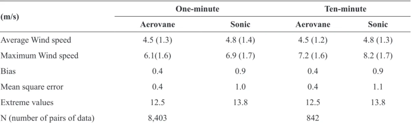
The data set was plotted in dispersion graphics with adjusted linear regression for one and ten-minute time interval (Fig. 2 and 3, respectively). For the one and ten-minute average wind speed (Fig. 2a and 3a), it can be noticed that the values are very consistent with high values of r2 (both are 0.99). In general, the sonic measurements
are higher than the actual sensors used to measure the wind speed. The difference between them increases with the velocity, but it is roughly 4% plus an additional constant value (0.2 m/s). This represents 0.3 m/s for typical values of 4.0 m/s (during the wet season) and 0.5 m/s for stronger winds around 10.0 m/s (characteristic of the dry season). The linear regressions adjusted are almost the same for both time intervals. For the maximum wind speed (Fig. 2b and 3b), the same behavior was obtained: the sonic measurements are higher than the aerovane and this difference increases with the wind speed. The differences are almost the double (around 1.0 m/s) from the average wind speed. The differences showed by Short and Wheeler (2006) using the same type of sensors at the Kennedy Space Center are very closed to the results obtained in this study, thus suggesting that both results may be due to the characteristics of the sensors.
Table 2: Statistics between the average and maximum wind speed (m/s) for the sensors Aerovane and Sonic Anemometer for one- minute and ten-minutes time interval.
(m/s) One-minute Ten-minute
Aerovane Sonic Aerovane Sonic
Average Wind speed 4.5 (1.3) 4.8 (1.4) 4.5 (1.2) 4.8 (1.3)
Maximum Wind speed 6.1(1.6) 6.9 (1.7) 7.2 (1.6) 8.2 (1.7)
Bias 0.4 0.9 0.4 0.9
Mean square error 0.4 1.0 0.4 1.1
Extreme values 12.5 13.8 12.5 13.8
N (number of pairs of data) 8,403 842
*The values in parentheses represent the standard deviation of that sample.
Figure 2: Comparison between average (a) and maximum wind speed (b) for one-minute time interval.
time interval, the peak of these distributions is different: for the average wind speed, the aerovane´s peak is one class prior to the sonic (Fig. 4a), increasing this difference for two classes for the maximum wind speed (Fig. 4b). The ten-minute time interval results also presented the same behavior. Each class interval represents 0.5 m/s of wind speed difference, and these situations is coherent with the statistics showed in Table 1 and Figures 2 and 3. For both cases, the wind speed distribution is close to a normal (Gaussian) statistic distribution. Gisler (2009), using a different data set (winds observations from anemometric tower at ASC from the period of 1995 until 1999), showed that the wind low may be represented by a normal/Gaussian distribution.
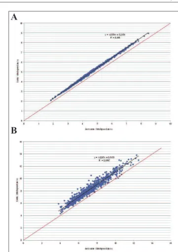
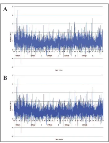
In order to analyze the time evolution of the difference between the two sensors, a time series for the average and maximum wind speed is showed in Figure 6 for one-minute time interval and at Figure 7 for ten-one-minute time interval. For most of the cases, the sonic measurements are higher than the aerovane. For the average wind speed, the difference ranged from -0.1 m/s to +1.0 m/s for one-minute and from +0.2 m/s up to +0.6 m/s for ten-one-minute time interval. These results for the maximum wind speed
Figure 3: Comparison between average (a) and maximum wind speed (b) for ten-minute time interval.
A
B
A
B
Figure 4: Frequency distribution for average (a) and maximum (b) wind speed for one-minute time interval.
ranged from -1.5 m/s to +4.5 m/s and from -0.1 to +3.3 m/s for one and ten-minute time interval, respectively.
CONCLUDING REMARKS AND FINAL COMMENTS
A
B
Figure 5: Frequency distribution for average (a) and maximum (b) wind speed for ten-minute time interval.
Figure 6: Time series of the difference between the average (a) and maximum wind speed (b) for one-minute time interval.
A
B
A
B
Figure 7: Time series of the difference between the average (a) and maximum (b) wind speed for ten-minute time in-terval.
As a draft procedure to joint the past (aerovane´s measurements) and the future (sonic´s measurement) data set, a ixed value (0.5 m/s for the average wind speed and 1.0 m/s for the maximum wind speed) must be added to the past data set in order to have it normalized with the new equipment. Additionally, an comparison between the sensors in a wind tunnel is highly desired in order to fulill this analysis, as well as other measurements during different meteorological conditions (wet season) and several heights.
ACKNOWLEDGMENTS
The author would like to acknowledge the entire team involved in the ield campaign from Operação Murici II, especially the meteorological technician Jorge Yamasaki, who prepared some of the statistics presented.
REFERENCES
Altino, K.M.; Barbré Jr., R.E., 2009, “Applications of Meteorological Tower Data at Kennedy Space Center”, 1st
Fisch, G., 1999, “Características do Peril Vertical do Vento no Centro de Lançamento de Foguetes de Alcântara (CLA)”, Revista Brasileira de Meteorologia, Vol. 14, No. 1, pp. 11-21.
Fisch, G., 2009, “The Atmospheric Boundary Layer: Concepts and Measurements”, In: Moreira, D.M. and Vilhena, M.T. (org.), “Air Pollution and Turbulence: Modelling and Applications”, CRC Press, Boca Ratton, US, pp. 3-19.
Gisler, C.A.F., 2009, “Análise do Peril do Vento na Camada Limite Supericial e Sistemas Meteorológicos Atuantes no Centro de Lançamento de Alcântara”, Dissertação de Mestrado em Meteorologia. 2009-05-25. [citado 24 fev 2010]. Available at: <http://urlib.net/sid. inpe.br/MCT-m18@80/2009/04.24.12.33>
Guedes, R. L; Oyama, M. D., 2004, “Aspectos observacionais das oscilações intra-sazonais de intensidade do vento em Alcântara usando ondeletas: análise preliminar”, In: XIII Congresso Brasileiro de Meteorologia, Meteorologia e o desenvolvimento sustentável. Anais de Fortaleza, CE, CD-ROM.
Johnson, D.L., 2008, “Terrestrial Environment (Climatic) Criteria Guidelines for Use in Aerospace Vehicle Development”, 2008 Revision (NASA/TM—2008– 215633). D.L. Johnson, Editor, Marshall Space Flight Center, Marshall Space Flight Center, Alabama, December 2008. [cited 2 jul 2009], available at: http://ntrs.nasa.gov/ search.jsp.
Leão, R.C., 2009, “Ajuste do Peril Vertical de Vento no Centro de Lançamento de Alcântara com dados obtidos por torre anemométrica e radiossondagem no Centro de Lançamento de Alcântara (CLA)”, Dissertação de Mestrado em Engenharia Aeroespacial, Instituto Tecnológico de Aeronáutica, 85 p.
Pereira, E.I. (Org.), 2002, “Atlas Climatológico do Centro de Lançamento de Alcântara”, Relatório de Desenvolvimento ACA/RT 01/01 GDO-000000/B0047, 186 p.
Plate, E.J., “Engineering Meteorology: Fundamentals of Meteorology and their application to problems in environmental and civil engineering”, Elsevier Scientiic Publishing Company, Studies in Wind Engineering and Industrial Aerodynamics, Vol 1, 733 p.
Roballo, S.T., Fisch, G., 2008, “Escoamento atmosférico no Centro de Lançamento de Alcântara (CLA): Parte I- aspectos observacionais”, Revista Brasileira de Meteorologia, Vol. 23, No. 4, pp. 510-519. doi: 10.1590/ S0102-77862008000400010.
Short, D. A., Wheeler, M.M., 2006, “RSA/Legacy Wind Sensor Comparison. Part II: Eastern Range”, NASA Contract Report CR 2006-214205, 26 p, 2006. [cited 2010, mar 18] Available at http://science.ksc.nasa.gov/amu/.