Anomalous effect in Schumann resonance phenomena observed in Japan, possibly associated with the Chi-chi earthquake in Taiwan

SRef-ID: 1432-0576/ag/2005-23-1335 © European Geosciences Union 2005

Annales

Geophysicae

Anomalous effect in Schumann resonance phenomena observed in

Japan, possibly associated with the Chi-chi earthquake in Taiwan

M. Hayakawa1, K. Ohta2, A. P. Nickolaenko1,3, and Y. Ando1

1_{The University of Electro-Communications, Department of Electronic Engineering, 1-5-1 Chofugaoka, Chofu Tokyo}

182-8585, Japan

2_{Chubu University, Department of Electronics Engineering, 1200 Matsumoto-cho Kasugai, Aichi, 487-8501, Japan} 3_{Institute of Radiophysics and Electronics, Academy of Sciences of Ukraine, Kharkov, Ukraine}

Received: 6 December 2004 – Revised: 14 February 2005 – Accepted: 22 February 2005 – Published: 3 June 2005

Abstract. The Schumann resonance phenomenon has been monitored at Nakatsugawa (near Nagoya) in Japan since the beginning of 1999, and due to the occurance of a severe earthquake (so-called Chi-chi earthquake) on 21 September 1999 in Taiwan we have examined our Schumann resonance data at Nakatsugawa during the entire year of 1999. We have found a very anomalous effect in the Schumann resonance, possibly associated with two large land earthquakes (one is the Chi-chi earthquake and another one on 2 November 1999 (Chia-yi earthquake) with a magnitude again greater than 6.0). Conspicuous effects are observed for the larger Chi-chi earthquake, so that we summarize the characteristics for this event. The anomaly is characterized mainly by the unusual increase in amplitude of the fourth Schumann resonance mode and a significant frequency shift of its peak frequency (∼1.0 Hz) from the conventional value on theBy magnetic

field component which is sensitive to the waves propagat-ing in the NS meridian plane. Anomalous Schumann reso-nance signals appeared from about one week to a few days before the main shock. Secondly, the goniometric estima-tion of the arrival angle of the anomalous signal is found to coincide with the Taiwan azimuth (the unresolved dual di-rection indicates toward South America). Also, the pulsed signals, such as the Q-bursts, were simultaneously observed with the “carrier” frequency around the peak frequency of the fourth Schumann resonance mode. The anomaly for the second event for the Chia-yi earthquake on 2 November had much in common. But, most likely due to a small mag-nitude, the anomaly appears one day before and lasts until one day after the main shock, with the enhancement at the fourth Schumann resonance mode being smaller in ampli-tude than the case of the Chi-chi earthquake. Yet, the other characteristics, including the goniometric direction finding result, frequency shift, etc., are nearly the same. Although the emphasis of the present study is made on experimental aspects, a possible generation mechanism for this anomaly

Correspondence to: M. Hayakawa

(hayakawa@whistler.ee.uec.ac.jp)

is discussed in terms of the ELF radio wave scattered by a conducting disturbance, which is likely to take place in the middle atmosphere over Taiwan. Model computations show that the South American thunderstorms (Amazon basin) play the leading role in maintaining radio signals, leading to the anomaly in the Schumann resonance.

Keywords. Ionosphere (Ionospheric disturbances) – Elec-tromagnetics (Wave propagation) – Meteorology and atmo-spheric dynamics (Lightning)

1 Introduction

Electromagnetic phenomena associated with seismic activ-ity have been extensively discussed, e.g. see the compre-hensive monographs on these subjects by Hayakawa and Fujinawa (1994), Hayakawa (1999), and Hayakawa and Molchanov (2002). Particularly intriguing are short-term electromagnetic phenomena, which appear either as precur-sory signatures or as effects around the earthquake date.

30

60

120

150 210

240 300

330

90

180 270

0

(a)

30

60

120

150 210

240 300

330

90

180 270

0

(b)

Nakatsugawa

Taiwan

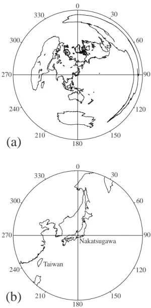
Fig. 1.(a)Relative location of our ULF/ELF observatory in Nakat-sugawa and Taiwan in the form of world map with our ULF obser-vatory located at the origin. The thunderstorm-active region in Asia is the South-east Asia, which is close to the direction of Taiwan from our ULF/ELF observatory, and South America (Amazon) is in the opposite direction.(b)The enlarged map indicating the relative location of Japan and Taiwan.

Hayakawa et al. (1996); Molchanov and Hayakawa (1998); Molchanov et al. (1998); Hayakawa et al. (2004); and Hayakawa (2004) to study the morphological characteristics of seismo-ionospheric perturbations, as well as the gener-ation mechanism of such seismo-ionospheric perturbgener-ations in terms of the lithosphere-atmosphere-ionosphere coupling (Hayakawa et al., 2004). However, we do not think that the number of convincing seismo-electromagnetic phenom-ena is sufficient enough to persuade the seismologists who are still very skeptical about the presence of these seismo-electromagnetic phenomena.

In this paper we will present new records, which are com-pletely different from those already reported in the literature.

The anomalous behaviour of the Schumann resonance signal was observed in Japan, which seems to be associated with the earthquakes in Taiwan. The Schmann resonance (SR) is a natural global electromagnetic phenomenon excited by light-ning discharges mainly in the tropical region (Nickolaenko and Hayakawa, 2002). Natural oscillations are used in this paper as a radio probe of the lower ionosphere, just like the sub-ionospheric VLF/LF transmitter signals.

2 ULF/ELF observing system in Nakatsugawa, Japan

Our observatory is located at a very low-noise site in Nakat-sugawa (geographic coordinates; 35.4◦N, 137.5◦E), near Nagoya in Japan. The three magnetic field components (Bx,

By andBz)in the ULF/ELF range have been continuously

measured since the beginning of 1999 at this observatory by means of three orthogonal induction coil magnetome-ters. The definition of Bx is given as follows. Bx means

the geomagnetically NS component of the wave magnetic field, which can be measured by the induction magnetometer whose axis is aligned with the NS direction. So, the com-ponent of Bx is sensitive to the waves propagating in the

EW direction. Then, theBy component is sensitive to the

waves propagating in the meridian plane. The waveform data from each channel are digitized with a sampling frequency of 100 Hz, and are saved on a hard disk every six hours. The details of this ULF/ELF observing system has already been extensively described in Ohta et al. (2001).

3 One year (1999) SR analysis and the Chi-chi earth-quake in Taiwan

Figure 1 illustrates the relative location of our ULF/ELF ob-servatory (Nakatsugawa), Taiwan (where the Chi-chi earth-quake took place), and thunderstorm-active regions like Southeast Asia and South America (Amazon). We under-stand that the thunderstorm-active area in Southeast Asia is located approximately in the direction of Taiwan from our ULF/ELF observatory and also the American source (Ama-zon) is nearly in the opposite direction.

(20 km). The circle enclosing the three successive earth-quakes indicates the occurrence of the earthearth-quakes in the land. Another anomaly in the SR phenomena was identified for the last isolated earthquake on 2 November 1999 (Chia-yi earthquake). The indication of the circles on Sch4 stands for the detection of the anomaly at the fourth SR mode, with no effect on the third SR mode (Sch3).

Below we provide you with the detailed description of the anomalous SR phenomena which are possibly associated with this Chi-chi earthquake. Lastly, we show briefly some details of the SR phenomena for the last earthquake.

4 Anomalous behaviors in SR phenomena observed at Nakatsugawa

The SR resonance takes place in the Earth-ionosphere cav-ity driven by electromagnetic radiations from lightning dis-charges, which are concentrated in the tropical region (Nick-olaenko and Hayakawa, 2002). The fundamental frequency isf1∼7.8 Hz (the first SR mode, n=1) and higher

harmon-ics are located atf2∼13.9 (n=2), f3∼20.0 (n=3), f4∼26.0

(n=4 Hz), etc. Of course, we know that the SR intensity (not only fundamental, but also higher modes) depends on the source-observer distance. However, when an observer is located at middle latitude (like in Japan), the fundamental mode n=1 is known to be usually the strongest, and the in-tensity is known to decrease with the mode number. We now describe the anomalous SR behaviors which are likely to be associated with the Chi-chi earthquake.

4.1 Resonance structure

Figure 3 shows the temporal evolution of the SR intensity, seen from the top to the bottom, the intensity at the funda-mental (f1)and those at the harmonics (f2,f3andf3),

ob-served at Nakatsugawa. The magnetic component used is

By (measuring the magnetic field component in the EW

di-rection, being sensitive to the waves propagating in the NS direction (nearly in the magnetic meridian plane)). A very similar tendency has been confirmed for anotherBx

compo-nent, as well, so that it is not illustrated here. As is already known (Nickolaenko and Hayakawa, 2002; Sentman,1995), the resonance frequency (fn)is very stable (for example, the

possible range inf1is, at maximum, 0.15 Hz), but the

reso-nance frequencies in our case are found to exhibit much more significant shifts (we will show this later), so that the band-width in Fig. 3 is taken to be rather large, such as fn±2.5 Hz, and the intensity integrated over this bandwidth is plotted in Fig. 3. The unit of integrated intensity in the ordinate is the same for all resonance frequencies. The period covers only the month of September 1999, but we have to mention that the level before and after this month remains nearly the same as the background level at each resonance frequency (fn).

It is very surprising that the integrated intensity atf4is

ex-tremely enhanced as compared with those atf1,f2 andf3

during the period of 15 September to the end of September

㪰㪼㪸㫉㩷㪑㩷㪈㪐㪐㪐 㪰㪼㪸㫉㩷㪑㩷㪈㪐㪐㪐 㪰㪼㪸㫉㩷㪑㩷㪈㪐㪐㪐 㪰㪼㪸㫉㩷㪑㩷㪈㪐㪐㪐

㪈㪆㪈 㪈㪆㪈 㪈㪆㪈

㪈㪆㪈 㪉㪆㪈㪉㪆㪈㪉㪆㪈 㪊㪆㪈㪉㪆㪈 㪊㪆㪈㪊㪆㪈㪊㪆㪈 㪋㪆㪈㪋㪆㪈 㪌㪆㪈㪋㪆㪈㪋㪆㪈 㪌㪆㪈㪌㪆㪈㪌㪆㪈 㪍㪆㪈㪍㪆㪈㪍㪆㪈 㪎㪆㪈㪍㪆㪈 㪎㪆㪈 㪏㪆㪈㪎㪆㪈㪎㪆㪈 㪏㪆㪈㪏㪆㪈 㪐㪆㪈㪏㪆㪈 㪐㪆㪈㪐㪆㪈㪐㪆㪈 㪈㪇㪆㪈㪈㪇㪆㪈㪈㪇㪆㪈㪈㪇㪆㪈 㪈㪈㪆㪈㪈㪈㪆㪈㪈㪈㪆㪈㪈㪈㪆㪈 㪈㪉㪆㪈㪈㪉㪆㪈㪈㪉㪆㪈㪈㪉㪆㪈 㪛㪸㫋㪼

㪛㪸㫋㪼㪛㪸㫋㪼 㪛㪸㫋㪼

㪎㪅㪍 㪎㪅㪍 㪎㪅㪍 㪎㪅㪍

㪍㪅㪊 㪍㪅㪊 㪍㪅㪊 㪍㪅㪊 㪌㪅㪊

㪌㪅㪊㪌㪅㪊

㪌㪅㪊 㪌㪅㪉㪌㪅㪉㪌㪅㪉㪌㪅㪉 㪍㪅㪋㪍㪅㪋㪍㪅㪋㪍㪅㪋

㪍㪅㪊 㪍㪅㪊 㪍㪅㪊 㪍㪅㪊

㪪㪺㪿㪋 㪪㪺㪿㪋㪪㪺㪿㪋 㪪㪺㪿㪋 㩷㩷㩿㪽㪋㪀 㩷㩷㩿㪽㪋㪀㩷㩷㩿㪽㪋㪀 㩷㩷㩿㪽㪋㪀

㪪㪺㪿㪊 㪪㪺㪿㪊㪪㪺㪿㪊 㪪㪺㪿㪊 㩷㩷㩿㪽㪊㪀 㩷㩷㩿㪽㪊㪀㩷㩷㩿㪽㪊㪀 㩷㩷㩿㪽㪊㪀

㩷㩷㪜㫈 㩷㩷㪜㫈㩷㩷㪜㫈 㩷㩷㪜㫈

Fig. 2. One-year (1999) summary of SR observations in

Nakat-sugawa and anomalous SR behaviors in possible association with two large land earthquakes in Taiwan. Dots on Sch4 mean that an anomaly is taking place at the fourth SR mode, and no dots on Sch3 mean that there is no effect at the third SR mode. An earthquake with a circle indicates the land earthquake, while an earthquake without a circle means that it occurs in the sea.

✁ ✁✂ ✁✄ ✁✄✂ ✁☎ ✁☎✂ ✁✆

✝✞✄ ✝✞✄✄ ✝✞☎✄ ✄✞✄

✟✠✡ ☛☞

✌ ✍☞ ✎ ✏ ✌ ✑ ✒ ✓ ✔

Fig. 3. Temporal evolution of the SR intensities (onBy)at the fun-damental (f1)and higher harmonics (f2,f3andf4)in September

1999. The intensities are the values integrated over a bandwidth of ±2.5 Hz at 8, 14, 20 and 25 Hz, respectively.

(about two weeks), which is very abnormal because the in-tensity atf4is normally much weaker than that at lowerfn

(n=1, 2, and 3) (Nickolaenko and Hayakawa, 2002). The in-tegrated intensity atf4is found to show a pronounced peak

starting on 15 September and decaying for a few days, with the next broad maximum with amplitude oscillation during the period of 22 to 28 September. We pay our greatest atten-tion tof4, but Fig. 3 shows that considerable deviations are

also seen in the amplitudes of other lower-order modes. Figure 4 illustrates the above temporal evolution for the sameBycomponent in a different form as the dynamic

㪇㪅㪇㪇 㪉㪌㪅㪇㪇 㪌㪇㪅㪇㪇

㪐㪆㪈 㪐㪆㪈㪈 㪐㪆㪉㪈 㪈㪇㪆㪈

㪛㪸㫐

㪝

㫉㪼㫈

㫌㪼㫅㪺㫐

㪲㪟

㫑㪴

-60 -40 -20 0 20 [dB]

Fig. 4. Temporal evolution of dynamic spectrum of the SR intensity

in September 1999. The intensity is indicated in color.

㪄㪊㪌 㪄㪊㪇 㪄㪉㪌 㪄㪉㪇 㪄㪈㪌 㪄㪈㪇 㪄㪌 㪇

㪇 㪌 㪈㪇 㪈㪌 㪉㪇 㪉㪌 㪊㪇 㪊㪌 㪋㪇 㪋㪌 㪌㪇

㪝㫉㪼㫈㫌㪼㫅㪺㫐㩷㪲㪟㫑㪴 㪠㫅

㫋㪼 㫅㫊 㫀㫋㫐 㩷㪲㪻 㪙㪴

㪙㫏 㪙㫐

㩿㪸㪀

㪄㪊㪌 㪄㪊㪇 㪄㪉㪌 㪄㪉㪇 㪄㪈㪌 㪄㪈㪇 㪄㪌 㪇

㪇 㪌 㪈㪇 㪈㪌 㪉㪇 㪉㪌 㪊㪇 㪊㪌 㪋㪇 㪋㪌 㪌㪇

㪝㫉㪼㫈㫌㪼㫅㪺㫐㩷㪲㪟㫑㪴 㪠㫅

㫋㪼 㫅㫊 㫀㫋㫐 㩷㪲㪻 㪙㪴

㪙㫏 㪙㫐

㩿㪹㪀

Fig. 5. Frequency spectra of SR on 10 September (normal

condi-tion)(a)and on 16 September (abnormal condition)(b). The two magnetic components (BxandBy) are shown.

the frequency is in a range up to 50 Hz. The wave intensity is indicated in the given color code. As seen from Fig. 4, the in-tensity of higher harmonics (f4)is extremely enhanced from

15 September to the end of September. Figure 5 illustrates the frequency spectra on two particular days; 10 September (normal condition) (LT=6 h−12 h) and on 15 September

(ab-11 12 13 14 15 16 17 18

Date in September, 1999 2

8 14 20 26 32

0 0.00025 0.0005 0.00075 0.001 0.00125 0.0015 0.00175 0.002 0.00225 Hx, Lehta, September 11-18, 1999

11 12 13 14 15 16 17 18

Date in September, 1999

2 8 14 20 26 32

0 0.00025 0.0005 0.00075 0.001 0.00125 0.0015 0.00175 0.002 0.00225 0.003 Hy, Lehta, September 11-18, 1999

Frequency [Hz]

Frequency [Hz]

Fig. 6. Corresponding dynamic spectra of the SR at the Lekhta

station (as a reference station) during the same September 1999.

normal condition) (LT=6 h−12 h), as observed by theBxand

By components. One notices easily the enhancement atf4,

with a significant frequency shift on both components. For comparison, we plot in Fig. 6 the corresponding SR phenom-ena observed at Lekhta (geographic coordinates; 64.43◦N, 33.97◦E), Karelia, Russia during the same period. We can-not find any significant anomalous behavior, especially in the fourth mode in Lekhta. The intensity is definitely decreas-ing with increasdecreas-ing mode number and also the resonance fre-quencies (fn)are found to be the conventional values. There

is a narrow line just below 26 Hz, but it is apparently an arti-ficial noise.

4.2 Shift in resonance frequencies, asymmetry in the reso-nance frequency forBx andBy components and

reso-nance intensity

We describe in more detail the anomalies in the SR. As is seen in Figs. 3, 4 and 5, the fourth harmonic (fn)is extremely

enhanced in the dynamic spectra. We have measured the frequency of the fourth harmonic (f4)on the two

horizon-tal magnetic field components (Bx andBy). As mentioned

before, one file has a duration of 6 h, so that we have in-tegrated the intensity over 6 h only to find the frequency of maximum intensity. Figure 7 illustrates this temporal varia-tion of the frequency (f4)on the two magnetic components

(By andBx)during the anomalous period of 15 September

to the end of September. The abscissa of Fig. 7 indicates the date (e.g. 15 means 15 September) and there are four di-visions in one day with file numbers 0, 1, 2 and 3 (e.g. 0 means 0−6 h LT, 1 means 6−12 h LT and so on). We con-tinue cover the same September 1999. We have to comment on the frequency resolution in estimating Fig. 7. We use the data length of 1,024×10 ms (∼10 s), so that the frequency resolution is 0.098 Hz and the time resolution is 10 s. Fig-ure 7 indicates that the central resonance frequency (f4)is

September for the magnetic componentBy, while the

cor-responding resonance frequency (f4) is found to be much

more stable than theBybehavior in such a way that the

res-onance frequency (f4) is found to be just around 26.3 Hz.

As compared with the previous experimental findings, see Nickolaenko and Hayakawa (2002) and recent measurements (Price and Melnikov, 2004), the resonance frequency for the

Bycomponent is found to be significantly lower than the

con-ventional value by 0.6−0.8 Hz. However, the resonance fre-quency for theBxcomponent is seen to be slightly (but

sig-nificantly) different from the conventional value by +0.3 Hz (+ means higher than the conventional value).

TheBy component in Fig. 7 is reflecting the wave

activ-ity propagating in the NS direction (nearly in the magnetic meridian plane), that is, thisBycomponent seems to be very

sensitive to the nearest Asian thunderstorm activity. It is ob-vious that the diurnal variation of the resonance frequency for theBycomponent exhibits a very clear diurnal variation

in such a way that we expect a minimum for the file num-bers 1 or 2; that LT=6−12 h or 12 h−18 h (corresponding to the Asian thunderstorm activity), and a maximum around midnight in LT (larger source-observer distance (for Ameri-can and AfriAmeri-can sources) by considering that the resonance frequency is closely related to the source-observer distance for the three sources (Nickolaenko and Hayakawa, 2002). This experimental diurnal variation is likely to be consistent with the theoretical expectation as given in Nickolaenko and Hayakawa (2002). Here we have to comment on the diur-nal variation for anotherBx component (which is sensitive

to the waves propagating mainly in the EW direction). A close inspection of Fig. 7 indicates that theBx component

in Fig. 7 seems to show the similar diurnal variation as for theBy component, but much less pronounced than for the

Bycomponents. Altogether these suggest that the abnormal

behaviors, as presented in this paper, are fundamentally sup-posed to be closely related to the thunderstorm activity in the tropical region.

How about the diurnal variation of the intensity atf4for

both magnetic components? Although not shown as a figure, we have found that the diurnal variation of the intensity is not so significant for both magnetic components (Bx and By).

This seems to be consistent with the previous experimental findings (Nickolaenko and Hayakawa, 2002).

4.3 Direction finding results

Because of the significant difference in the central frequen-cies of SR atf4 on the two magnetic components, the

go-niometer direction finding is performed for each component (Bx or By). When we perform the goniometric direction

finding to the SR phenomena anomaly observed for theBy

component, we first estimate the maximum intensity on the

Bycomponent with the previously-mentioned frequency

ev-ery 10 s and we perform the goniometric direction finding as is given in Hayakawa (1995) at those frequencies in a range from 25.1 to 26.0 Hz by using the radio ofBxandBy

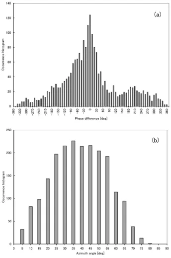
compo-nents. Figure 8a illustrates the occurrence histograms of the

㪉㪋㪅㪌 㪉㪌 㪉㪌㪅㪌 㪉㪍 㪉㪍㪅㪌 㪉㪎

㪐㪆㪈㪌 㪐㪆㪈㪍 㪐㪆㪈㪎 㪐㪆㪈㪏 㪐㪆㪈㪐 㪐㪆㪉㪇 㪐㪆㪉㪈 㪐㪆㪉㪉 㪐㪆㪉㪊 㪐㪆㪉㪋 㪐㪆㪉㪌 㪐㪆㪉㪍 㪐㪆㪉㪎 㪐㪆㪉㪏 㪐㪆㪉㪐 㪐㪆㪊㪇 㪛㪸㫐

㪝㫉 㪼㫈 㫌㪼 㫅㪺 㫐㩷 㪲㪟

㫑㪴 㪙㫏㩷㪲㪟㫑㪴㪙㫐㩷㪲㪟㫑㪴

Fig. 7. Detailed temporal evolutions of the fourth resonance

fre-quency (f4) on the two magnetic antennas (BxandBy) during the

same September.

phase difference between the componentsBx andBy (with

Byas the reference,By−Bx), indicating that the occurrence

number is well peaked around 0◦(suggesting the linear po-larization). This phase information enables us to adopt the principle of the goniometer to estimate the azimuthal direc-tion for the waves. Figure 8b is the result, which means that the waves are coming from the azimuth of 215◦with a rather wide distribution. This central direction is close to the di-rection of Taiwan (235◦) and that of the Asian thunderstorm source region and the American source (Amazon), as is seen from Fig. 1.

Figures 9a and b are the corresponding direction finding results for the Bx component. Figure 9a is the occurrence

histogram of the phase difference betweenBxandBy (with

Bxas the reference,Bx−By), which indicates a broad

distri-bution with a peak around∼60◦. Even in this situation we perform the goniometric finding, and the result is illustrated in Fig. 9b, which indicates∼90◦(measured eastward from the north). Probably there must be a significant polarization error in the estimation of azimuth in Fig. 9b (as is suggested in Hayakawa (1995)) because of a significant departure of the phase difference from 0◦_{. However, the source in Fig. 9b}

might be American (Amazon).

4.4 Associated ELF transients and ULF emissons

One notices the presence of ELF transients (Q bursts) in Fig. 4, which indicates the pulsive noises (or pulsive spectra) superimposed on the enhanced SR at f4 from 15

Septem-ber to the end of SeptemSeptem-ber. The occurrence of simultane-ous ELF transients is observed during the same period of enhanced SR intensity atf4 from 15 September to the end

㪇 㪉㪇 㪋㪇 㪍㪇 㪏㪇 㪈㪇㪇 㪈㪉㪇 㪈㪋㪇

㪄㪊 㪍㪇

㪄㪊 㪊㪇

㪄㪊 㪇㪇

㪄㪉 㪎㪇

㪄㪉 㪋㪇

㪄㪉 㪈㪇

㪄㪈 㪏㪇

㪄㪈 㪌㪇

㪄㪈

㪉㪇 _㪄㪐㪇 _㪄㪍㪇 _㪄㪊㪇 㪇 㪊㪇 㪍㪇 㪐㪇 _㪈㪉㪇 㪇_{㪈㪌 㪈㪏}㪇 _㪉㪈㪇 _㪉㪋㪇 _㪉㪎㪇 _㪊㪇㪇 _㪊㪊㪇 _㪊㪍㪇

㪧㪿㪸㫊㪼㩷㪻㫀㪽㪽㪼㫉㪼㫅㪺㪼㩷㪲㪻㪼㪾㪴 㪦

㪺㪺 㫌㫉 㫉㪼 㫅㪺 㪼㩷 㪿㫀 㫊㫋 㫆㪾 㫉㪸 㫄

㩿㪸㪀

㪇 㪌㪇 㪈㪇㪇 㪈㪌㪇 㪉㪇㪇 㪉㪌㪇

㪇 㪌 㪈㪇 㪈㪌 㪉㪇 㪉㪌 㪊㪇 㪊㪌 㪋㪇 㪋㪌 㪌㪇 㪌㪌 㪍㪇 㪍㪌 㪎㪇 㪎㪌 㪏㪇 㪏㪌 㪐㪇

㪘㫑㫀㫄㫌㫋㪿㩷㪸㫅㪾㫃㪼㩷㪲㪻㪼㪾㪴 㪦

㪺㪺 㫌㫉 㫉㪼 㫅㪺 㪼㩷 㪿㫀 㫊㫋 㫆㪾 㫉㪸 㫄

㩿㪹㪀

Fig. 8. (a)Occurrence histogram of the phase difference in a fre-quency range of 25.1∼26.0 Hz (withBy component as the refer-ence) and(b)the occurrence histogram of the obtained arrival di-rection (measured from north to east).

main frequency of our ELF transients in Fig. 4 is clearly not atf1, but just around thef4. Again, we have performed the

goniometric direction finding for those ELF transients, and we have found that the azimuthal direction of those ELF tran-sients is mainly distributed around 235◦(which is the direc-tion toward Taiwan). Figure 4 indicates, as well, the presence of the associated ULF transients which have already been extensively discussed for this Chi-chi earthquake by Ohta et al. (2001).

4.5 Repeatability

Now we want to add one more important point for this anomalous SR phenomena; repeatability of this anomaly. Al-though Fig. 3 indicates that the intensity variation at ∼f4

with a peak on 15 September and with decaying for a few days might be associated with the Chi-chi earthquake, we find an additional broad peak on 22 September to 26 Septem-ber (a little complicated, but seeming to be one event) in this figure. An aftershock of the Chi-chi earthquake is known to have taken place nearly at the same place at 8:53 JST on 26

㪇 㪈㪇 㪉㪇 㪊㪇 㪋㪇 㪌㪇 㪍㪇 㪎㪇 㪏㪇 㪐㪇 㪈㪇㪇

㪄㪊 㪍㪇

㪄㪊 㪊㪇

㪄㪊 㪇㪇

㪄㪉 㪎㪇

㪄㪉 㪋㪇

㪄㪉 㪈㪇

㪄㪈 㪏㪇

㪄㪈 㪌㪇

㪄㪈

㪉㪇 _㪄㪐㪇 _㪄㪍㪇 _㪄㪊㪇 㪇 㪊㪇 㪍㪇 㪐㪇 _㪈㪉㪇 㪇_{㪈㪌 㪈㪏}㪇 _㪉㪈㪇 _㪉㪋㪇 _㪉㪎㪇 _㪊㪇㪇 _㪊㪊㪇 _㪊㪍㪇

㪧㪿㪸㫊㪼㩷㪻㫀㪽㪽㪼㫉㪼㫅㪺㪼㩷㪲㪻㪼㪾㪴 㪦

㪺㪺 㫌㫉 㫉㪼 㫅㪺 㪼㩷 㪿㫀 㫊㫋 㫆㪾 㫉㪸 㫄

㩿㪸㪀

㪇 㪈㪇㪇 㪉㪇㪇 㪊㪇㪇 㪋㪇㪇 㪌㪇㪇 㪍㪇㪇 㪎㪇㪇 㪏㪇㪇 㪐㪇㪇 㪈㪇㪇㪇

㪇 㪌 㪈㪇 㪈㪌 㪉㪇 㪉㪌 㪊㪇 㪊㪌 㪋㪇 㪋㪌 㪌㪇 㪌㪌 㪍㪇 㪍㪌 㪎㪇 㪎㪌 㪏㪇 㪏㪌 㪐㪇 㪘㫑㫀㫄㫌㫋㪿㩷㪛㫀㫉㪼㪺㫋㫀㫆㫅㩷㪲㪻㪼㪾㪴

㪦 㪺㪺 㫌㫉 㫉㪼 㫅㪺 㪼㩷 㪿㫀 㫊㫆 㫋㫆 㪾㫉 㪸㫄

㩿㪹㪀

Fig. 9. The same as Fig. 8, expect for theBx component in the frequency range of 26.2–26.7 Hz.

September, which may suggest the peak on 22–26 September is closely associated with this aftershock. Of course, there may be a possibility that this broad peak might be the after-effect of the Chi-chi earthquake. We cannot say which inter-pretation may be plausible. However, it seems more likely by the description of the anomalous SR event for another large earthquake in Taiwan (as already shown in Fig. 2) that the first peak may be related to the Chi-chi earthquake and the second broad peak, its aftershock.

smaller than those for the Chi-chi earthquake, which might be related to its much smaller magnitude. Other character-istics (goniometric direction finding result, frequency shift, etc.) are found to be nearly the same as those for the Chi-chi earthquake.

5 Summary of the anomalous SR behavior, possible as-sociation with the Chi-chi earthquake and discussion on the generation mechanism

We can summarize the anomalous SR behaviors observed at Nakatsugawa prior to two large earthquakes which took place in Taiwan in September and November, 1999.

1. Unlike the usual situation of SR, the intensity of the fourth mode (∼f4) for the Chi-chi earthquake is

en-hanced at Nakatsugawa during the period from 15 September to the end of September 1999. Also, there is an enormous asymmetry in the resonance frequency (f4)for both magnetic components, Bx andBy. The

By component (sensitive to the wave coming from the

NS direction) andBxas well exhibit the enhancement at

f4, but the exact resonance frequency for theBx

compo-nent is about 1 Hz lower than the conventional value of 26.0 Hz, and the corresponding value for another mag-netic component (Bx)is slightly higher than the

conven-tional value by +0.3 Hz. This kind of SR anomaly was not seen in Lekhta, where the SR characteristics are ex-actly in the normal condition.

2. The arrival azimuth for the SR wave around 25.2 Hz mainly for theBycomponent is found to be∼250◦, very

close to the direction of Taiwan, while that for the SR wave at 26 Hz mainly for theBxcomponent, is found to

be directed forward South America (or Amazon). 3. Another important finding is the simultaneous

occur-rence of ELF transients, but their frequency is just aroundf4, very similar to the Q-burst as observed by

Ogawa et al. (1967). The direction finding for those ELF transients indicates that their azimuth is exactly in the direction of Taiwan.

This kind of rare case was also observed for another large (Chia-yi) earthquake in Taiwan (in November 1999) with characteristics similar to the Chi-chi case.

6 Discussion and interpretation

First, we have to discuss whether this kind of unusual behav-ior in SR is a natural phenomenon or not, and whether this anomaly is related to the Chi-chi earthquake. Assuming that this is a kind of artificial noise (like train noise), the emis-sion line must then be much narrower than our event. The Q factor of the fourth resonance (f4)in our case is of the order

of∼10, which is a further indication of natural phenomenon, though this value is nearly twice the conventional SR value

6:00 0 50

Frequenc

y [Hz]

12:00 JST

12:00 0 50

Frequenc

y [Hz]

18:00 JST

Fig. 10. Dynamic spectra of the SR at Nakatsugawa one day

be-fore the earthquake (2 November 1999) (i.e. 1 November 1999, JST=6:00–18:00), in which one notices an anomaly in the fourth resonance mode in possible association with the earthquake on 2 November 1999.

as given in Nickolaenko and Hayakawa (2002). Additional observational facts in support of this natural noise effect are (1) theBycomponent (also on theBxcomponent, but not so

prominent) exhibits a typical diurnal variation in resonance frequency at∼f4and (2) the direction finding for the

emis-sion at∼f4for theBycomponent shows that it is directed

in-cidentally toward the direction of Taiwan and also the direc-tion of America. The first observadirec-tional fact is strongly indi-cating that the source of this anomaly is likely to be the global thunderstorm-active region in Southeast Asia and America, which is observationally supported by the 2nd direction find-ing result. Therefore, we can conclude that this anomaly is a real typical SR phenomenon with anomalous behaviors.

The next problem is whether this anomaly in SR phenom-ena is really associated with the Chi-chi earthquake or not. The first point is that this anomaly in SR is taking place before the Chi-chi earthquake, which is not so convincing as a precursory effect of an earthquake. Of course, it may be possible for us to think it just as a coincidence. How-ever, we have shown the repeatability of this kind of SR anomaly again for another big earthquake in Taiwan. This would lend us some more convincing support to our suppo-sition that those anomalies are the consequence of the big earthquakes. Some other big earthquakes in Japan have pro-duced similar behaviour (of course, not exactly the same, but the higher harmonics had some abnormal behaviors), which will be our next paper, no effect was completely confirmed at Lekhta (Karelia, Russia). Further, smaller earthquakes with magnitudes less than 6.0 had no effect on the SR, as shown in Fig. 2, which may be an additional support that the anoma-lous SR phenomena might be earthquake-related.

(a) ASIA (Indonesia)

Observer

Disturbance

Source in Asia

1.73 Mm

5.5 Mm 2 Mm

3.77 Mm 1 Mm

3.9 Mm

(b) AFRICA

Observer

Disturbance Source Africa

13.3 Mm

13.45 Mm

2 Mm

(c) AMERICA

Observer

Disturbance

American Source

19 Mm

2x2.0 Mm

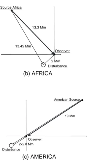
Fig. 11. Three thunderstorm regions (a) Asia (Indonesia), (b)

Africa and(c)America (Amazon) and the configurations of the di-rect path and that scattered at Taiwan are given for each source.

is known to be the fundamental frequency of SR (Ogawa et al., 1967; Nickolaemko and Hayakawa, 2002). The gener-ation of ULF emission has already been confirmed by Ohta et al. (2001) to have the goniometric direction toward wan. This might indicate an additional noise source in Tai-wan, which may be the precursory to the Chi-chi earthquake. How to explain various characteristics of the anomaly de-scribed in this paper, is poorly understood, so that we propose one possible hypothesis. The two important points of the SR anomaly and (1) the fourth resonance is extremely enhanced for theBycomponent and (2) a significant shift of the order

of a little less than 1.0 Hz for theBy component. When

tak-ing into account different properties, the source for the SR anomaly is highly likely to be the thunderstorm in the South-east Asia or in the South America (Amazon region). We initially assume that the ionosphere (or in the atmosphere) above the epicenter of the Chi-chi earthquake is perturbed, acting as a scatterer (or a reflector). We then think about three possible thunderstorm centers in Asia, Africa and America. The configurations for a direct path and the path scattered at Taiwan for those three sources are summarized in Fig. 11. In the case of the Asian source (Fig. 11a), the source-observer distance is 5.5 Mm, and the path difference between this di-rect path and the path scattered at Taiwan is about 0.4 Mm. The maximum effect (strongest wave interference effect) is expected when this path difference is equal toλ/2 (λ: wave-length). Then we obtainλ=0.8 Mm. Sinceλ=40 Mm at the first SR mode, the above wavelength is found to correspond to the 40/0.8=50 mode number, or to the frequency of ap-proximately 300 Hz. So, Asia is the poorest candidate for strong wave interference at∼f4.

We move on to the next source of Africa (Fig. 11b); source-observer distance=13 Mm, and the path difference be-tween the direct path and that scattered at Taiwan is 2.15 Mm. The maximum effect is reached when the path difference is equal toλ/2 and henceλ=4Mm. This means that the above wavelength corresponds to the 40/4=10 mode number, or to the frequency of about 60 Hz. So, Africa is found to be not good, but not so bad either. The last source of America is considered (Fig. 11c); the source-observer distance=19 Mm and the path difference between the direct path and the path scattered at (or reflected from) Taiwan=4 Mm. We can expect the maximum wave interference effect when this path differ-ence isλ/2, so that λ=8 Mm. This wavelength is found to correspond to the 40/8=5 mode number, or to the frequency of approximately 32 Hz. In this sense, the American source (Amazon) is found to be the most reasonable candidate for the source position. Fortunately, the direction (azimuth) of Taiwan is nearly in the same direction to the Amazon, so that we can think of a very simple situation. The observer re-ceives both the direct signal from the American source and the signal reflected from the ionospheric perturbation located at Taiwan, as is seen is Fig. 11c.

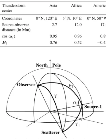
Table 1. Coordinates, distances to the observer, and geometrical

parameters of the model.

Thunderstorm Asia Africa America

center

Coordinates 0◦N, 120◦E 5◦N, 10◦E 0◦N, 50◦W

Source-observer 2.7 12.0 17.2

distance (in Mm)

cos (αi) 0.95 0.96 0.89

Mi 0.76 0.52 −0.43

North Pole

Observer

Source-1

Scatterer γ

γ θ

α

1 1 1

Fig. 12. Configuration of our scattering problem.

independent of the mutual positions of the field source, ob-server and disturbance. The vertical electric field is a sum of the direct (primary) (E1)and scattered (E2)waves:

E=E1+E2. (1)

The direct (or primary) wave is defined simply by the formula (Eqs. (4.16) and (4.18) in Nickolaenko and Hayakawa (2002).

E1(ω)= M(ω)

4ha2_ε

iν (ν+1) ω

Pν[cos(π−θi)]

sinπ ν . (2)

Hereω is the wave angular frequency,M(ω) is the source current moment, ν(ω) is the propagation constant depend-ing on the frequency,h, the ionospheric height,a,the Earth’s radius and theε, dielectric constant of free space. Here we use the linear frequency dependence,ν(f )=(f−2)/6−i·f/70

(Nickolaenko and Hayakawa, 2002).Pν(cosθ )is the

Legen-dre function, and the angular distanceθi acquires the values

θ1,θ2, orθ3, corresponding to the sources placed in Asia,

Africa and America in Fig. 11. Figure 12 shows the geom-etry of this scattering problem. It is convenient to introduce individual fractional contributions from the ionospheric dis-turbance into the field arriving from different sources:

B= E2

E1

=

R

sinθ dθ dϕ Qiδ Cν2

4 sinπ ν Pν[cos(π −θi)]

, (3)

where

Qi =ν (ν +1) Pν[cos(π −γi )] Pν[cos(π −γ )]

,

−MP_ν1[cos(π −γi )] Pν1[cos(π −γ )] (4)

where P_ν1(cosθ )is the associated Legendre function, γ is the angular distance from the observer to disturbance, γi

is the distance from the disturbance to the given source in Asia, Africa, or America. The geometrical param-eter of differentiation is found from the following rela-tion, M=∂γi

∂γ=

sinθicosγi·cosαi−sinγicosθi

sinγ (see Nickolaenko

and Hayakawa, 2002). We suppose that the ionospheric modification locally changes the propagation parameter

δC_ν2=δ1−ν(ν+1)

(ka)2

=−iδZ_kh(k,propagation constant of free space and δZ, the change in surface impedance) (Nicko-laenko, 1994), and this latter has a symmetric “Gaussian” angular distribution:

δ C_ν2= 1C_ν2exp

_cosβ−1

d2

. (5)

Here1C_ν2is the maximum disturbance,βis the angular dis-tance from the center of ionospheric modification to the point of integration, andd is the characteristic size of the modifi-cation. One readily obtains the following formula after in-tegrating Eq. (3) in the above case of a compact, localized non-uniformity:

B= E2

E1

= π d

2

2

1 C_ν2·Qi

sin(π ν) Pν[cos(π −θi)]

. (6)

We use the following model in our computations. The observer is located at Nakatsugawa, Japan (35.45◦_{N and}

137.3◦E). The disturbance is placed over Taiwan whose ge-ographic coordinates are 24◦N and 122◦E, and its character-istic sized corresponds to 1000 km (d=π/20). We suppose that one of three global thunderstorm centers drives the SR signal. The coordinates and relevant parameters of geometry are listed in Table 1. In our computations at lower ELF SR frequencies for the possible earthquake disturbance we for-mally increased the disturbance of the complex cosine by a factor of (40/π) in our comparison, by using the value used at the frequency of 75 Hz (Pappert, 1981):1 C_ν2=40_πRa·Cν2.

The factorRawas introduced for interpretations of the

night-time disturbances observed experimentally in the ELF signal from the US Navy transmitter (Wisconsin Test Facility), and its value is Ra=0.13617−i·10.6949 (see Nickolaenko and

0 0.2 0.4 0.6 0.8 1 1.2 0 0.2 0.4 0.6 0.8 1 1.2

5 8 11 14 17 20 23 26 29 32 Frequency Hz

0 0.2 0.4 0.6 0.8 1 1.2

5 8 11 14 17 20 23 26 29 32 Frequency Hz

0 0.5 1 1.5 2 2.5 3

America

Africa

Asia

Direct Wave

Disturbed

Direct Wave

Direct Wave

Disturbed

Disturbed

|Er( f a.u. | B( f ) |

America

Africa

Asia

)|

Fig. 13. Left panel shows the computational results on the

fre-quency dependence for three thunderstorm centers. The right panel indicates the frequency dependences of the vertical electric field ex-pected at our observatory for three sources (from the top to the bot-tom; America, Africa and Asia). A thin line refers to the direct wave without the effect of ionospheric perturbation, while a thick line, the corresponding result for the disturbed case (with the iono-spheric perturbation over Taiwan).

6 12 18 24 30 36 42 8

14 20 26 32

Disturbed Regular

-14 -8 -6 -5 -3 -1 1 3

Frequency [Hz]

Fig. 14. Model dynamic spectrum of SR when a disturbance abruptly appears over Taiwan (at UT=12 h)

.

clear that the implication of an increasedRa factor simply

raised the effect, so that a problem could happen with validity of the perturbation theory method employed in our computa-tions. The results of computations are shown in Fig. 13. The left frame of Fig. 13 illustrates the frequency dependence of the dimensionless field disturbance, see Eq. (6), computed for the sources located in Asia, Africa, and America. One may see that the highest relative disturbance is connected to the Asian source and is observed around the 20-Hz frequency (third SR mode). The plots in the left frame of Fig. 13 pro-vide the “general picture” of the wave scattering, and one has to remember that the function|B(f)|may become large not only when the scattered field (denominator) is large, but also when the direct wave is small, e.g. at the nodal distance. This latter instance exactly the case for the source in Asia; see the lower frame in the right column of the plots in Fig. 13. The right plots in Fig. 13 show the spectra of the sole direct wave (no ionospheric disturbance) shown in a black line with cor-responding spectra in the presence of the modification, given in a red line marked as “Disturbed”. The lowest right frame

depicts the data computed for the Asian source. One may see that the undisturbed field has a minimum around the 20-Hz frequency. Therefore, the relevant peak appeared in the left frame for the Asian source. The spectra show that this source might produce a noticeable disturbance only around the sec-ond SR mode. The right-hand side plots of Fig. 13 indicate that only American thunderstorms are well positioned, caus-ing a two-fold increase in the spectral amplitude at frequen-cies aroundf4, as was already qualitatively described before.

The non-uniformity over Taiwan cannot increase the ampli-tudes of the waves arriving from other global thunderstorm centers. As the possible conclusion, the presence of an iono-spheric perturbation over Taiwan and the wave interference between the direct wave and that scattered from the iono-spheric perturbation at Taiwan, act together as a frequency filter, which should be multiplied with the conventional SR frequency spectrum in which the intensity is decreasing with the increase in mode number. This hypothesis is likely to ac-count for the major two points of our discovery (an enhance-ment at∼f4and a possible shift inf4). As seen in Fig. 13,

the seismo-ionospheric perturbation is likely to influence the lower harmonic as well, but we will not discuss this in any detail.

As the global lightning activity drifts around the planet during the day, a question arises: “Why is the increase in the field amplitude observed all through the day?” The drifting activity must produce the effect varying in time. The contro-versy might be resolved in the following way. Long-term SR observations in the horizontal magnetic field indicate that the natural signal is a sum of two components: one of them is sta-ble in time, forming a “podium” for the time-varying signal; see, e.g. SR records presented in Price and Melnikov (2004). We also know that there are two components; correspond-ingly the non-polarized and polarized signals (Nickolaenko et al., 2004). The time varying polarized part is associated with the electromagnetic radiation from the compact light-ning activity. The stable podium or non-polarized component originates from the “background” thunderstorms that cover the whole globe: they occur everywhere and at any time. Pulsed signals from such strokes arrive at an observer along the azimuth, ranging from 0 to 2π π, and merge into a non-coherent depolarized noise. Thus, we may accept that any thunderstorm center “works” all through the day, with activ-ity increasing by 30–50% during the local afternoon hours, so that the amplitude of SR never decreases substantially dur-ing the day.

The SR background signals permanently arrive at the Nakatsugawa observatory from all directions during the whole day, However, the “podium” signals coming from the American thunderstorms are reflected and enhanced by the ionospheric irregularity located over Taiwan. Thus, the field enhancement by the non-uniformity is observed all through the day in the vicinity of the fourth SR mode with minor am-plitude variations.

Hz, and the logarithm of the field intensity is shown by ink-ing. (do you mean shading?) The scale bar is given on the right side of the figure. Horizontal dashed grid lines indicate the usual positions of SR peaks in the spectrum. Vertical grid lines mark the 6-h intervals. The record of two days duration was modeled. There is no ionospheric perturbation during the first 12 h in the model dynamic spectrum, and regular di-urnal variations are present there with SR peaks observed as a regular succession of horizontal lines. The form of spec-trum abruptly changes after the ionosphere is modified over Taiwan (the choice of disturbance parameters is described below). The parts of the maps are marked as “regular” and “disturbed”. As one may see, the general behavior found ex-perimentally is pertinent to our model computations. The oc-currence of Q bursts atf4is apparently due to the enhanced

propagation characteristics at∼f4 because of the presence

of seismo-ionospheric perturbations at Taiwan. The source is the same as the SR, but from a giant lightning in America. We here comment on why no significant effect at Lekhta was observed. The geometry of the direct and reflected paths toward Lekhta indicates that there is no such lucky situation (as given in this paper): no backscatter. The theory (Nick-olaenko and Hayakawa, 2002) indicates that at ELF only the overhead disturbance or a backscattering from a nearby disturbance may produce a noticeable effect. In this sense Lekhta is a remote place and we expect no backscattering signal.

Emergence of ionospheric perturbations prior to a large earthquake has already been evidenced by means of subiono-spheric VLF/LF propagation anomalies (Hayakawa et al., 1996; Molchanov et al., 1998). Because these subiono-spheric VLF/LF signals are known to be reflected from the lowest ionosphere (D region at day and lower E layer at night), it is already believed that the lowest ionosphere is perturbed a few days to about a week before large earth-quakes. Our recent study with the use of over-horizon VHF signals has indicated the presence of atmospheric (altitude ∼a few tens of km) perturbations about one week before the earthquakes (Fukumoto et al., 2001). ELF propaga-tion, including SR and ELF transients, is connected to two characteristic heights (h1 and h2) (Greifinger and Greifin-ger, 1978). The first altitude h1 is the height where the dis-placement current at a given frequency becomes equal to the conductivity current. It is the height at which the at-mosphere becomes a conducting medium (the electric field does not penetrate to the altitudes above h1). The h2 is the height where the fields change from wave-like to diffusion-like (only the magnetic field component reaches the altitude h2). The characteristic value of h1 at SR frequencies is ap-proximately h1∼50 km, while h2∼90 km (Nickolaenko and Hayakawa, 2002; Mushtak and Williams, 2002). Therefore, we can understand that the height range responsible for ELF propagation is perturbed in association with earthquakes, tak-ing into account the experimental or observational evidence of seismo-atmospheric and -ionospheric perturbations men-tioned before. The scale of the perturbation in the upper ionosphere is estimated as radius R (in km)=exp (M), where

M is the magnitude (Ruzhin and Depeuva, 1996). This yields R ∼2000 km for the magnitude of the Chi-chi earthquake (M=7.6), which means that atmospheric and seismo-ionospheric perturbations have the spatial scale of, at least, one Mm. These perturbations seem to be ready to reflect the ELF waves just around the epicenter of the Chi-chi earth-quake (in Taiwan) to be observed at the observatory. Liu et al. (2000) have studied thef0F2 for this Chi-chi earthquake,

and have found that the precursors appeared 1−6 days prior to this earthquake in the form of the recordedf0F2 decrease

below its associated lower bound. This means that some kind of anomaly is surely occurring in the ionosphere. Of course, the generation mechanism of seismo-ionospheric perturba-tions is not well established, but Hayakawa et al. (2004) have suggested a few possible mechanisms.

Lastly, we comment on the geomagnetic activity during the relevant period, because it may be possible that the geo-magnetic activity may influence the SR anomaly. Though not shown as a figure, the geomagnetic activity is not severely disturbed, so that the present SR anomaly is likely to have nothing to do with the geomagnetic activity.

Finally, we can suggest the lithospheric source. Kulchit-sky et al. (2004) have performed the detailed computations of ULF/ELF waves in the complicated lithospheric structure. We have to try to find any resonance effects in the litho-spheric waveguide (or cavity).

Acknowledgements. This study is partly supported by the

Mit-subishi Foundation and Japan Society of Promotion of Science (#15403012), to which we are grateful.

Topical Editor T. Pulkkinen thanks K. Hattori and another ref-eree for their help in evaluating this paper.

References

Fukumoto, Y., Hayakawa, M., and Yasuda, H.: Investigation of over-horizon VHF radio signals associated with earthquakes, Natural Hazards Earth System Sci., 1, 127–136, 2001.

Greifinger, C. and Greifinger, P.: Approximate method for deter-mining ELF eigen-values in the Earth-ionosphere waveguide, Radio Sci., 13, 831–837, 1978.

Hattori, K.: ULF geomagnetic changes associated with large earth-quake, Terr. Atmos. Ocean. Sci., 15, 329–360, 2004.

Hayakawa, M. and Fujinawa, Y.: Electromagnetic Phenomena Re-lated to Earthquake Prediction, Terra Sci. Pub. Co., Tokyo, 667, 1994.

Hayakawa, M.: Whistlers, in “Handbook of Atmospheric Electro-dynamics”, Volland, H.(Ed.), 1, 155–193, CRC Press, Boca Ra-ton, 1995.

Hayakawa, M., Molchanov, O. A., Ondoh, T., and Kawai, E.: The precursory signature effect of the Kobe earthquake on VLF subionospheric signals, J. Comm. Res. Lab., Tokyo, 43, 169– 180, 1996.

Hayakawa, M.: “Atmospheric and Ionospheric Electromagnetic Phenomena Associated with Earthquakes”, TERAPPUB, Tokyo, 966, 1999.

Hayakawa, M., Hattori, K., and Ando, Y.: Natural electromagnetic phenomena and electromagnetic theory, Inst. Electr. Engs. Japan (IEEJ), Trans. Fundamentals and Materials, 124, 1, 72–79, 2004. Hayakawa, M.: Is earthquake prediction possible by means of electromagnetic phenomena associated with earthquakes?, IEEJ, Trans. Fundamentals and Materials, 124, 1, 3–4, 2004.

Hayakawa, M. and Hattori, K.: Ultra-low-frequency electromag-netic emissions associated with earthquakes (Invited paper), in “Special Issue on Recent Progress in Electromagnetic Theory and Its Application”, Inst. Electr. Engrs. Japan, Trans. Funda-mentals and Materials, 124, 1101–1108, 2004.

Hayakawa, M., Molchanov, O. A., and NASDA/UEC team: Sum-mary report of NASDA’s earthquake remote sensing frontier project, Special Issue on “Seismo Electromagnetics and Related Phenomena”, Hayakawa, M., Molchanov, O. A., Biagi, P., and Vallianatos, F. (Eds.), Phys. Chem. Earth, 29, 617–626, 2004. Kulchitsky, A., Ando, Y., and Hayakawa, M.: Numerical analysis

on the propagation of ULF/ELF signals in the lithosphere with highly conductive layers, Phys. Chem. Earth, 29, 551–557, 2004. Liu, J. Y., Chen, Y. I., Pulinets, S. A., Tsai, Y. B., and Chuo, Y. J.: Seismo-ionospheric signatures prior to M≥6.0 Taiwan earth-quakes, Geophys. Res. Lett., 27, 3113–3116, 2000.

Molchanov, O. A., Hayakawa, M., Ondoh, T., and Kawai, E.: Pre-cursory effects in the subionospheric VLF signals for the Kobe earthquake, Phys. Earth Planet. Inter., 105, 239–248, 1998. Molchanov, O. A. and Hayakawa, M.: Subionospheric VLF signal

perturbations, possibly related to earthquakes, J. Geophys. Res., 103, 17 489–17 504, 1998.

Mushtak, V. C. and Williams, E. R.: ELF propagation parameters for uniform models of the Earth-ionosphere waveguide, J. At-mos. Solar-terr. Phys., 64, 1989–2001, 2002.

Nickolaenko, A. P.: ELF radio wave propagation in a locally non-uniform Earth-ionosphere cavity, Radio Sci., 29, 1187–1199, 1994.

Nickolaneko, A. P. and Hayakawa, M.: “Resonances in the Earth-ionosphere Cavity”, Kluwer Acad. Pub., Dordrecht, 380, 2002. Nickolaenko, A. P., Rabinowicz, L. M., Shvets, A. V., and

Scheko-tov, A. Yu.: Polarisation characteristics of low frequency reso-nances, Izvestija VUZov, Radiofizika, XLVII, (in Russian), 267– 291, 2004.

Ogawa, T., Tanaka, Y., Fraser-Smith, A. C., and Gendrin, R.: Worldwide simultaneity of a Q-burst in the Schumann resonance frequency range, J. Geomagn. Geolectr., 19, 377–384, 1967. Ohta, K., Umeda, K., Watanabe, N., and Hayakawa, M.: ULF/ELF

emissions observed in Japan, possibly associated with the Chi-chi earthquake, Natural Hazards Earth System Sci., 1, 37–42, 2001.

Pappert, R. A.: Effect of a large patch of sporadic E on night-time propagation at lower ELF, J. Atmos. Terr. Phys., 42, 417–425, 1981.

Price, C. and Melnikov, A.: Diurnal, seasonal and inter-annual vari-ations in the Schumann resonance parameters, J. Atmos. Solar-terr. Phys., 66, 1179–1185, 2004.

Ruzhin, Yu. Ya. and Depueva, A. Kh.: Seismoprecursors in space as plasma and wave anomalies, J.Atmos. Electr., 16, 3, 271–288, 1996.