Probability assessment on the recurring Meishan earthquake in central Taiwan with a new non-stationary analysis

(1)

NHESSD

2, 4831–4856, 2014

Non-stationary earthquake

probability assessment

J. P. Wang and X. Yun

Title Page

Abstract Introduction

Conclusions References

Tables Figures

◭ ◮

Back Close

Full Screen / Esc

Printer-friendly Version Interactive Discussion

Discussion

P

a

per

|

Discus

sion

P

a

per

|

Discussion

P

a

per

|

Discussion

P

a

per

|

Nat. Hazards Earth Syst. Sci. Discuss., 2, 4831–4856, 2014 www.nat-hazards-earth-syst-sci-discuss.net/2/4831/2014/ doi:10.5194/nhessd-2-4831-2014

This discussion paper is/has been under review for the journal Natural Hazards and Earth System Sciences (NHESS). Please refer to the corresponding final paper in NHESS if available.

Probability assessment on the recurring

Meishan earthquake in central Taiwan

with a new non-stationary analysis

J. P. Wang and X. Yun

Department of Civil and Environmental Engineering, The Hong Kong University of Science and Technology, Kowloon, Hong Kong

Received: 31 March 2014 – Accepted: 18 May 2014 – Published: 31 July 2014

Correspondence to: J. P. Wang ([email protected])

(2)

NHESSD

2, 4831–4856, 2014

Title Page

Tables Figures

◭ ◮

Back Close

Full Screen / Esc

Discussion

P

a

per

|

Discus

sion

P

a

per

|

Discussion

P

a

per

|

Discussion

P

a

per

Abstract

From theory to experience, earthquake probability should be increasing with time as far as the same fault is concerned, rather than being a stationary process or independent of the date of the last occurrence. With a new non-stationary model, we evaluated the earthquake probability associated with the Meishan fault in central Taiwan, a growing 5

concern to the local community given a relatively short return period reported (i.e., around 160 years). The analysis shows that on the condition that the earthquake has not recurred by the end of year 2014, the earthquake probability in the next 50 years could be around 0.3 (mean value), with a 95 % confidence interval from 0.26 to 0.36.

1 Introduction 10

In 1906, anML=7.1 earthquake, later referred to as the Meishan earthquake, struck central Taiwan and caused severe damage around the region. Recently, the return period of such events was reported at 162 years (Wang et al., 2012), and the relatively short return period makes the Meishan fault a growing concern to the local community. Under the circumstance, a few studies focusing on earthquake potential and seismic 15

hazard associated with the recurring Meishan earthquake were reported (Wu et al., 2009; Wang et al., 2012, 2013), with the same objective to mitigate earthquake risk around the region close to the active fault.

The Poisson process is commonly used for assessing earthquake probability (e.g., Weichert, 1980; Ang and Tang, 2007; Ashtari Jafari, 2010). By definition, the approach 20

is a “memory-less” model (Devore, 2008), meaning that the probability is a function of the length of time only, but being independent of the date of the last occurrence. How-ever, such a “memory-less” process seems not reflecting the reality very well because earthquake occurrence should be somehow related to the date of the last occurrence. For example, it should be very unlikely for the 2011 Tohoku earthquake in Japan to 25

(3)

NHESSD

2, 4831–4856, 2014

Title Page

Tables Figures

◭ ◮

Back Close

Full Screen / Esc

Discussion

P

a

per

|

Discus

sion

P

a

per

|

Discussion

P

a

per

|

Discussion

P

a

per

|

Given the “shortcoming” of the stationary Poisson model, a few non-stationary mod-els were proposed for earthquake probability assessment, such as renewal modmod-els and Markov models (Hagiwara, 1974; Veneziano and Cornell, 1974; Nishioka and Shah, 1980; Savy et al., 1980; Kiremidjian and Anagnos, 1984). But similar to the Poisson model, somehow those non-stationary models were also developed from an empirical 5

perspective, but not on the basis of earthquake mechanisms like the elastic rebound theory (Reid, 1910; Keller, 1996).

Given the Meishan fault in central Taiwan a growing concern to the local community, this paper is aimed at evaluating the earthquake probabilities with a new non-stationary analysis. Different from others, the key to the new model is to analyze the stress on 10

the fault plane at a given time, then comparing it to the failure stress to evaluate the earthquake probability at that time. In addition to the methodology, this study applied the non-stationary approach to the Meishan fault in central Taiwan, estimating that the probability is around 0.3 for the Meishan earthquake to recur within the next 50 years.

2 Overview of the Meishan fault 15

In 1906, anM_L=7.1 earthquake was occurring near Meishan Township in central Tai-wan, killing about three thousand people at that time. Because the earthquake was near Meishan Township in central Taiwan, later the fault and the earthquake were named after the location as the Meishan fault and the Meishan earthquake, respec-tively. After the earthquake, field investigation showed that the surface rupture was 20

around 15 km, with a fault scarp as large as 3 m (Lin et al., 2008).

Especially after the 1999 Chi-Chi earthquake, the Central Geological Survey Taiwan (CGST) has conducted a variety of investigations on the active faults in Taiwan. The investigations included field survey, geophysical testing, GPS monitoring, etc. After the investigation, the data such as earthquake return period and fault slip rate were 25

(4)

NHESSD

2, 4831–4856, 2014

Title Page

Tables Figures

◭ ◮

Back Close

Full Screen / Esc

Discussion

P

a

per

|

Discus

sion

P

a

per

|

Discussion

P

a

per

|

Discussion

P

a

per

analysis, and Wang and Wu (2014) used those earthquake magnitudes and return periods to conduct a risk assessment for active faults in Taiwan.

3 The Poisson process and earthquake probability

Given earthquake occurrences following the Poisson model, the probability for the next event to recur by timet∗ is considered following the exponential distribution, with a cu-5

mulative density function (CDF) as follows (Ang and Tang, 2007):

Pr(T ≤t∗;v)=1−e−vt∗ (1)

wherev is the mean rate. For example, given a return period of 162 years, the mean rate is equal to 1/162 year−1.

10

Using this model, we can estimate the earthquake probability associated with the Meishan fault. On the condition that the earthquake has not occurred by the end of 2013 since 1906 (the very last occurrence), the earthquake probability in 2014 is calculated as follows givenv=1/162 year−1:

Pr(year 2013< T ≤year 2014|T >year 2013)

=Pr(107 years< T ≤108 years) Pr(T >107 years) =

Pr(T ≤108 years)−Pr(T ≤107 years) 1−Pr(T ≤107 years)

=(1−e

−108/162

)−(1−e−107/162)

1−(1−e−107/162₎ =0.006

(2) 15

On the other hand, assuming the earthquake has not occurred by the end of 2023, the earthquake probability in year 2024 is:

(5)

NHESSD

2, 4831–4856, 2014

Title Page

Tables Figures

◭ ◮

Back Close

Full Screen / Esc

Discussion

P

a

per

|

Discus

sion

P

a

per

|

Discussion

P

a

per

|

Discussion

P

a

per

|

=Pr(117 years< T ≤118 years) Pr(T >117 years) =

Pr(T ≤118 years)−Pr(T ≤117 years) 1−Pr(T ≤117 years)

=(1−e

−118/162

)−(1−e−117/162)

1−(1−e−117/162₎ =0.006

(3)

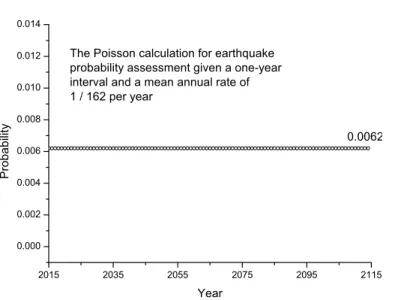
From the two calculations, we can see the “memory-less” e_ffect of the stationary model: the time-invariant probability (i.e., 0.006) was only governed by the length of time (i.e., 5

one-year interval), but irrelevant to the year either in 2014 or 2024. To demonstrate the stationary model more clearly, Fig. 1 shows the time-invariant probability for each year of the next 100 years, on the condition that the event has not occurred by the end of the previous year.

4 A new non-stationary model

10

4.1 Overview of Mohr–Coulomb failure criterion

The Mohr–Coulomb failure criterion is a model to describe a material’s mechanical behavior subject to external stresses (Pariseau, 2007), and it is commonly applied to rock mechanics, soil mechanics, etc. Figure 2 is a schematic diagram illustrating the essentials of the model. Basically, as the stresses represented by a Mohr circle that is 15

(6)

NHESSD

2, 4831–4856, 2014

Title Page

Tables Figures

◭ ◮

Back Close

Full Screen / Esc

Discussion

P

a

per

|

Discus

sion

P

a

per

|

Discussion

P

a

per

|

Discussion

P

a

per

4.2 Tectonic stress evolution between earthquakes

It is understood that the ongoing tectonic activities are the main reason for the in-creases in tectonic stresses with time, causing rock failures with the release of ac-cumulated strain energy in a form of the so-called earthquake (Reid, 1910). With the theory, this section shows stress evolutions between two major earthquakes associ-5

ated with a specific fault, in order to assess earthquake probabilities at a given time since the last recurrence.

After a major earthquake, two principle stresses in the vertical and horizontal direc-tions should be adjusted to a similar level, governed by the coefficient of lateral earth pressureK in rock. That is, the horizontal stressσhat that time should be equal toK σv 10

(whereσv is vertical stress). Therefore at that time, the stresses can be represented like Mohr circle A in Fig. 2. Given the region subject to tectonic compression, the hor-izontal stress σh could increase from Point A to Point B like Mohr circle B in Fig. 2, and at that time rock failure or earthquake is not expected. But as the compression continues, eventually the Mohr circle would be in contact with the failure envelope as 15

σ1 orσh keeps increasing to Point C, and at that time a recurrence earthquake could be expected.

Based on the theory of the Mohr–Coulomb failure criterion, σ1 at failure (Point C in Fig. 2) can be expressed as a function ofσ3 (vertical stress in this case) and two strength parameters of the shearing plane (or the fault plane), as follows (Pariseau, 20

2007):

σ1_failure=σ3

1+sinφ

1−sinφ

+2c·cosφ

1−sinφ (4)

wherecandφare the cohesion and friction angle, respectively.

As a result, the earthquake probability int∗years after the last recurrence becomes 25

(7)

NHESSD

2, 4831–4856, 2014

Title Page

Tables Figures

◭ ◮

Back Close

Full Screen / Esc

Discussion

P

a

per

|

Discus

sion

P

a

per

|

Discussion

P

a

per

|

Discussion

P

a

per

|

not; therefore the earthquake probability can be formulated as follows:

Pr(earthquake aftert∗years since last recurrence)=1−Pr(σ1_t∗≤σ_{1_failure}) (5) In this governing equation,σ1_t∗ and σ_{1_failure} are two random variables, and their for-mulations and calculations are detailed in the following.

5

4.3 Annual stress increment

To estimateσ1 int ∗

years after the last recurrence, we introduce annual stress incre-ment (ASI) to formulateσ1that is a function of time:

σ1_t∗=σ_{1_}_t

0+t

∗_·_ASI ₍₆₎

10

whereσ1_t₀ denotes the horizontal stress right after the major earthquake. Since it is

equal toK σvas mentioned previously, the equation can be rewritten as:

σ1_t∗=K σ_v+t∗·ASI (7) where vertical stress σ_v is associated with the weight of overburden rock above the 15

failure plane, or fault plane, or the depth of earthquakes.

4.4 The mean and standard deviation of ASI

The next step of the earthquake probability assessment is to determine the mean value and standard deviation of annual stress increment, then to determine the probability distribution of the major principle stress (i.e., σ1) at a given time after the last occur-20

(8)

NHESSD

2, 4831–4856, 2014

Title Page

Tables Figures

◭ ◮

Back Close

Full Screen / Esc

Discussion

P

a

per

|

Discus

sion

P

a

per

|

Discussion

P

a

per

|

Discussion

P

a

per

the mean value of ASI (i.e.,µASI) can be derived as follows:

E[σ1_˜t]=E[K σv+t˜·ASI]=σ1_failure

⇒E[ASI]=σ1_failure−K σv ˜

t =µASI

(8)

whereE[ ] denotes the mean value in the derivations.

By contrast, it is very difficult to characterize the standard deviation of ASI (denoted 5

assASI) without the studies on the region’s tectonic stress increment and its variability in time. Under the circumstances, our best estimates on the variability of ASI are from 0.25 to 1.0 in terms of COV (=standard deviation/mean value), and their influence on the earthquake probability assessments is discussed in the following with a parametric analysis.

10

As a result, given the COV of ASI equal ton, its standard deviation can be expressed withnand its mean value (Eq. 8) as follows:

sASI=n·µASI=

n·(σ1_failure−K σv) ˜

t (9)

4.5 The mean and standard deviation ofσ₁_{at time}t∗

15

With the derivations in Eqs. (6)–(9), we can estimate the mean and standard deviation ofσ1at timet

∗

since the last recurrence. Combining Eqs. (7) and (8), the mean value ofσ1at timet

∗

(denoted asµσ1_t∗) can be derived as follows:

σ1_t∗=K σ_v+t∗·ASI

⇒E[σ_{1_}_t∗]=E[σ₃+t∗·ASI]=K σ_v+t∗·E[ASI]

=K σv+

t∗·(σ1_failure−K σv) ˜

t

(10)

(9)

NHESSD

2, 4831–4856, 2014

Title Page

Tables Figures

◭ ◮

Back Close

Full Screen / Esc

Discussion

P

a

per

|

Discus

sion

P

a

per

|

Discussion

P

a

per

|

Discussion

P

a

per

|

Similarly, the standard deviation ofσ1at timet ∗

(denoted assσ1_t∗) can be derived as follows with the standard deviation of ASI given in Eq. (9):

σ1_t∗=K σ_v+t∗·ASI

⇒V

σ1_t∗=V[K σ_v+t∗·ASI]=t∗2·V[ASI]=t∗2·s_ASI2

⇒sσ1_t∗= q

V

σ1_t∗=t∗·s_ASI=

t∗·n· σ1_failure−K σv

˜

t

(11)

whereV[ ] denotes variance in the derivations, which is the square of standard devia-5

tion.

In addition to the mean value and standard deviation, the probability distribution is also needed for estimating the probability density function (PDF) ofσ1 at a given time. Without any reference available, the study presumes this variable follows the normal distribution, as a few probabilistic assessments adopted this model in the analyses 10

when relevant information is not available (Abramson et al., 2002; Wang and Huang, 2013).

4.6 Summary of the methodology

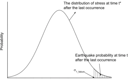
Figure 3 is a schematic diagram summarizing the new framework for earthquake prob-ability assessments. With the PDF ofσ1_t∗, the earthquake probability int∗years after 15

the last occurrence, i.e., 1−Pr(σ1_t∗< σ_{1_failure}), can be simply calculated with the fun-damentals of probability and statistics. To sum up, the new non-stationery analysis estimating recurrence earthquake probabilities associated with a specific fault is gov-erned by a total of seven parameters, i.e., return period (˜t), rock strength parameters (cand φ), unit weight (γ), earthquake depth (d), coefficient of lateral earth pressure 20

(K), and the variability of annual stress increment (n).

(10)

NHESSD

2, 4831–4856, 2014

Title Page

Tables Figures

◭ ◮

Back Close

Full Screen / Esc

Discussion

P

a

per

|

Discus

sion

P

a

per

|

Discussion

P

a

per

|

Discussion

P

a

per

coefficient of lateral earth pressure in rock was considered from 0.2 to 0.5 (Gercek, 2007). As mentioned previously, given no references regarding the variability of annual stress increment around the study region, we presumed that it ranged from 0.25 to 1.0 as our best estimate in this study.

5 Case study: earthquake probability associated with the Meishan fault 5

With the new non-stationary model, a case study was presented in this section to esti-mate the recurring Meishan earthquake probabilities in each year of the next 100 years, on the condition that the major earthquake has not recurred by the end of the previous year.

On the use of those central values and n=0.25 (see Table 1), Fig. 4 shows the 10

earthquake probability for each year of the next 100 years, given that the earthquake has not occurred by the end of the previous year. The analysis shows that the non-stationary probability would increase from 0.0008 (in 2015) to 0.019 (in 2115) in the next 100 years, in contrast to a time-invariant probability of 0.006 from using the sta-tionary Poisson model.

15

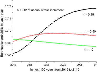
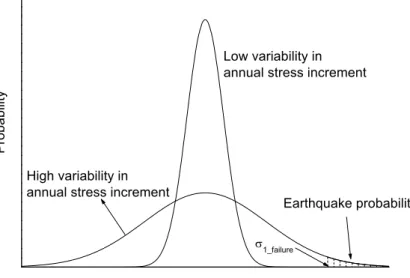
Figure 5 shows the earthquake probability on three scenarios withn=0.25, 0.5 and 1.0. Based on the parametric study, the variability of annual stress increment could have a substantial influence on the earthquake probability. Figure 6 shows a schematic diagram to help explain such a variation. For the case with low ASI variability, the distribution is rather concentrated, and therefore the earthquake probability [i.e., 1−

20

Pr(σ1_t∗< σ_{1_failure})] is relatively small. By contrast, for the case with high ASI variability, the distribution of σ1_t∗ that is less concentrated could lead to a higher earthquake probability at that time.

It is worth noting that the result given in Figs. 4 and 5 is in terms of conditional probability rather than cumulative probability, and this is the reason why the curves are 25

(11)

NHESSD

2, 4831–4856, 2014

Title Page

Tables Figures

◭ ◮

Back Close

Full Screen / Esc

Discussion

P

a

per

|

Discus

sion

P

a

per

|

Discussion

P

a

per

|

Discussion

P

a

per

|

probability is to compare the new analysis with the Poisson model on the same basis, in which the probability calculated refers to conditional probability.

6 Monte Carlo simulation

The estimates given in Figs. 4 and 5 were on a deterministic basis for using those central values in the analysis (see Table 1). In this section, we introduce a probabilistic 5

analysis to estimate the earthquake probability, in which the parameters were consid-ered as random variables that are uniformly distributed within the best-estimate range (see Table 1). Because the analyses would become much more complex and the ana-lytical solution might not be available, we employed Monte Carlo Simulation (MCS) to solve the problem like many other probabilistic studies (e.g., Wang et al., 2010, 2012; 10

Moghaddasia et al., 2011).

Basically, the MCS of this study is to generate random parameters (e.g., n,φ, . . . ) within the best-estimate range at first, then substituting them in the governing equa-tions of the non-stationary model to compute a random earthquake probability. With the randomization repeated for a number of times, a series of earthquake probabili-15

ties become available for calculating the mean probability or confidence interval, the fundamentals of Monte Carlo Simulation.

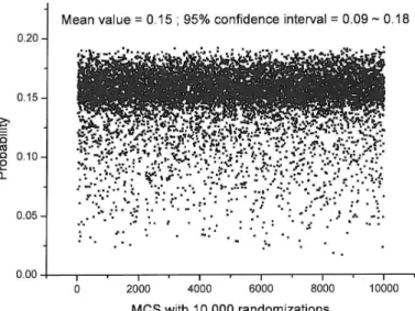
For example, Fig. 7 shows the MCS with a sample size of 10 000 to estimate the earthquake probability associated with the Meishan fault in years 2015∼2040, on the condition that the earthquake has not recurred by the end of year 2014 since the last 20

occurrence in 1906. Accordingly, the earthquake probability within the next 25 years is about 0.15, with a 95 % confidence interval from 0.09 to 0.18. Besides, the simulation shows that the estimate in this case should be asymmetrically distributed, with a longer tail in the left-hand side of its probability density function.

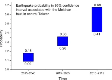
Using the new non-stationary model and Monte Carlo Simulation, Fig. 8 shows an-25

(12)

NHESSD

2, 4831–4856, 2014

Title Page

Tables Figures

◭ ◮

Back Close

Full Screen / Esc

Discussion

P

a

per

|

Discus

sion

P

a

per

|

Discussion

P

a

per

|

Discussion

P

a

per

in 2015∼2065 is about 0.3 with a 95 % confidence interval from 0.26 to 0.36, and the probability could increase to 0.53 (with a 95 % confidence interval from 0.41 to 0.68), as far as a longer time interval of 100 years was concerned.

7 Discussions

7.1 Earthquake is stationary or non-stationary? 5

Although earthquake occurrence should be non-stationary from theory to experience, a recent statistical study somehow provided the support that earthquake occurrence should follow a stationary Poisson process by analyzing the seismicity around Taiwan (Wang et al., 2014). But when closely comparing the statistical study with this study, we can find that the problems targeted are different: this study is focusing on a non-10

stationary model associated with a specific fault, and the recent statistical analysis was to examine whether a regional seismicity should follow the Poisson distribution. There-fore, although using the Poisson distribution to model regional seismicity was supported with earthquake statistics, the conclusion is irrelevant to this study about a new non-stationary model for earthquake probability assessments as far as a given active fault 15

is concerned, which should be increasing with time and should not be independent of the date of the last occurrence.

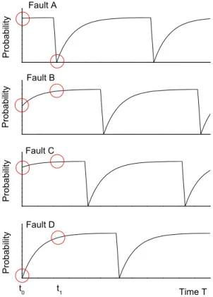
Figure 9 is a schematic diagram that helps explain the relationship between the two different problems. For each fault, the recurring earthquake should be a non-stationary process, with earthquake probability reset at the time while a major earthquake is re-20

curring, then increasing with time until the next recurrence. By contrast, the seismicity in a region would become stationary after combining many non-stationary processes. Take Fig. 9 for example, the sum of the probability atT =t0 should be similar to that atT =t₁, although the earthquake probability atT =t₀could be very low for Fault D, in contrast to a very low probability atT =t1for Fault A.

(13)

NHESSD

2, 4831–4856, 2014

Title Page

Tables Figures

◭ ◮

Back Close

Full Screen / Esc

Discussion

P

a

per

|

Discus

sion

P

a

per

|

Discussion

P

a

per

|

Discussion

P

a

per

|

The relationship can be simply explained with an analogy of a patron-and-bank prob-lem: for each patron (analogy to each fault), going to the bank is a non-stationary process, with the probability increasing with time since the last visit. But for the bank (analogy to the seismicity), it is a stationary process with the number of patrons that is more or less the same in any time, after combining that many non-stationary processes 5

from each patron.

7.2 Earthquake is very difficult to predict

Given the recent major earthquakes unpredicted, indeed earthquake prediction is very challenging with our limited understandings of the nature. As a result, like many earth-quake studies, this study is to propose a new perspective in earthearth-quake occurrence 10

analyses, but not to claim it is a perfect solution to earthquake prediction. However, it must be noted that the motivation and contribution of this study is to analyze the non-stationary earthquake occurrence with a new non-stationery model, an improvement over the use of the Poisson calculation in earthquake probability assessment, and the key scope of this study.

15

8 Conclusions

This study presents a new non-stationary analysis for earthquake probability assess-ments associated with a specific fault. The basics of the analysis are to estimate the probability distribution of the shear stress on the fault plane at a given time, then com-paring it to the failure stress.

20

(14)

NHESSD

2, 4831–4856, 2014

Title Page

Tables Figures

◭ ◮

Back Close

Full Screen / Esc

Discussion

P

a

per

|

Discus

sion

P

a

per

|

Discussion

P

a

per

|

Discussion

P

a

per

0.0008 (in 2015) to 0.019 (in 2115) in the next 100 years, on the condition that the earthquake has not recurred by the end of the previous year.

In addition, given the recurring Meishan earthquake has not occurred by the end of 2014, the earthquake probability in the next 50 years is about 0.3 (with a 95 % confi-dence interval from 0.26 to 0.36), on the basis of the new non-stationary model and 5

a probabilistic analysis using Monte Carlo Simulation.

Acknowledgements. We appreciate the valuable comments from Editor D. Keefer, making the submission much improved in so many aspects.

References

Abramson, L. W., Lee, T. S., Sharma, S., and Boyce, G. M.: Slope Stability and Stabilization 10

Methods, John Wiley & Sons, Inc., NJ, USA, 2002.

Ang, A. H. S. and Tang, W. H.: Probability Concepts in Engineering: Emphasis on Applications to Civil and Environmental Engineering, 2nd Edn., John Wiley & Sons, Inc., NJ, 199–202, 2007.

Ashtari Jafari, M.: Statistical prediction of the next great earthquake around Tehran, J. Geodyn., 15

49, 14–18, 2010.

Au, S. K., Wang, Z.-H., and Lo, S.-M.: Compartment fire risk analysis by advanced Monte Carlo simulation, Eng. Struct., 29, 2381–2390, 2007.

Cheng, C. T., Chiou, S. J., Lee, C. T., and Tsai, Y. B.: Study on probabilistic seismic hazard maps of Taiwan after Chi-Chi earthquake, Journal of GeoEngineering, 2, 19–28, 2007. 20

Devore, J. L.: Probability and Statistics for Engineering and the Sciences, Brooks/Cole, Boston, Massachusetts, 2008.

Gercek, H.: Poisson’s ratio values for rocks, Int. J. Rock Mech. Min., 44, 1–13, 2007.

Hagiwara, Y.: Probability of earthquake occurrence as obtained from a Weibull distribution anal-ysis of crustal strain, Tectonophysics, 23, 313–318, 1974.

25

Keller, E. A.: Environ. Geol., 7th Edn., Prentice Hall, Inc., NJ, 176–178, 1996.

(15)

NHESSD

2, 4831–4856, 2014

Title Page

Tables Figures

◭ ◮

Back Close

Full Screen / Esc

Discussion

P

a

per

|

Discus

sion

P

a

per

|

Discussion

P

a

per

|

Discussion

P

a

per

|

Lin, C. W., Lu, S. T., Shih, T. S., Lin, W. H., Liu, Y. C., and Chen, P. T.: Active faults of central Taiwan, Special Publication of Central Geological Survey, Taipei, Taiwan, 21, 148, 2008 (in Chinese with English Abstract).

Lin, C. W., Chen, W. S., Liu, Y. C., and Chen, P. T.: Active faults of eastern and southern Taiwan, Special Publication of Central Geological Survey, Taipei, Taiwan, 23, 178, 2009 (in Chinese 5

with English Abstract).

Moghaddasia, M., Cubrinovskia, M., Chaseb, J. G., Pampanina, S., and Carra, A.: Effects of soil–foundation–structure interaction on seismic structural response via robust Monte Carlo simulation, Eng. Struct., 33, 1338–1347, 2011.

Nishioka, T. and Shah, H. C.: Application of the Markov chain on probability of earthquake 10

occurrences, Proceedings of the Japanese Society of Civil Engineering, 1, 137–145, 1980. Pariseau, W. G.: Design Analysis in Rock Mechanics, Taylor & Francis/Balkema, 450–459,

2007.

Reid, H. F.: The mechanics of the earthquake, the California Earthquake of April 18, 1906, Re-port of the State Investigation Commission, Carnegie Institution of Washington, Washington 15

DC, 2, 1910.

Savy, H. B., Shan, H. C., and Boore, D. M.: Nonstationary risk model with geophysical input, J. Struct. Div. ASCE, 106, 145–164, 1980.

Veneziano, D. and Cornell, C. A.: Earthquake models with spatial and temporal memory for en-gineering seismic risk analysis, Research Report R74–78, Department of Civil Enen-gineering, 20

Massachusetts Institute of Technology, Cambridge, Massachusetts, 1974.

Wang, J. P. and Huang, D.: Deterministic seismic hazard assessments for Taiwan considering non-controlling seismic sources, B. Eng. Geol. Environ., 73, 635–641, doi:10.1007/s10064-013-0491-6, 2013.

Wang, J. P. and Wu, M. H.: Risk assessments on active faults in Taiwan, B. Eng. Geol. Environ., 25

doi:10.1007/s10064-014-0600-1, in press, 2014.

Wang, J. P., Lin, C. W., Taheri, H., and Chen, W. S.: Impact of fault parameter uncertainties on earthquake recurrence probability by Monte Carlo simulation – an example in central Taiwan, Eng. Geol., 126, 67–74, 2012.

Wang, J. P., Huang, D., and Chang, S. C.: Assessment of seismic hazard associated with the 30

(16)

NHESSD

2, 4831–4856, 2014

Title Page

Tables Figures

◭ ◮

Back Close

Full Screen / Esc

Discussion

P

a

per

|

Discus

sion

P

a

per

|

Discussion

P

a

per

|

Discussion

P

a

per

Wang, J. P., Huang, D., Chang, S. C., and Wu, Y. M.: New evidence and perspective to the Poisson process and earthquake temporal distribution from 55,000 events around Taiwan since 1900, Natural Hazards Review, 15, 38–47, 2014.

Wang, Y., Cao, Z., and Au, S. K.: Practical reliability analysis of slope stability by advanced Monte Carlo simulations in a spreadsheet, Can. Geotech. J., 48, 162–172, 2010.

5

Weichert, D. H.: Estimation of the earthquake recurrence parameters for unequal observation periods for different magnitudes, B. Seismol. Soc. Am., 70, 1337–1346, 1980.

Wu, C. F., Lee, W. H. K., and Huang, H. C.: Array deployment to observe rotational and trans-lational ground motions along the Meishan fault, Taiwan: a progress report, B. Seismol. Soc. Am., 99, 1468–1474, 2009.

(17)

NHESSD

2, 4831–4856, 2014

Title Page

Tables Figures

◭ ◮

Back Close

Full Screen / Esc

Discussion

P

a

per

|

Discus

sion

P

a

per

|

Discussion

P

a

per

|

Discussion

P

a

per

|

Table 1.Summary of the model parameters used in the analyses.

Parameters Earthquake Unit Cohesion Friction Return Ka nb

depth weight (MN m2) angle period

(km) (kN m−3) (degrees) (years)

Range 5∼15 25∼30 3.6∼22.7 22∼46 – 0.2∼0.5 0.25∼1.0

Central value 10 27.5 13.2 34 162 0.35 –

a_K

(18)

NHESSD

2, 4831–4856, 2014

Title Page

Tables Figures

◭ ◮

Back Close

Full Screen / Esc

Discussion

P

a

per

|

Discus

sion

P

a

per

|

Discussion

P

a

per

|

Discussion

P

a

per

2015 2035 2055 2075 2095 2115 0.000

0.002 0.004 0.006 0.008 0.010 0.012 0.014

The Poisson calculation for earthquake probability assessment given a one-year interval and a mean annual rate of 1 / 162 per year

0.0062

P

robabi

lity

Year

(19)

NHESSD

2, 4831–4856, 2014

Title Page

Tables Figures

◭ ◮

Back Close

Full Screen / Esc

Discussion

P

a

per

|

Discus

sion

P

a

per

|

Discussion

P

a

per

|

Discussion

P

a

per

|

(20)

NHESSD

2, 4831–4856, 2014

Title Page

Tables Figures

◭ ◮

Back Close

Full Screen / Esc

Discussion

P

a

per

|

Discus

sion

P

a

per

|

Discussion

P

a

per

|

Discussion

P

a

per

The distribution of stress at time t* after the last occurrence

Earthquake probability at time t* after the last occurrence

σ_{1_failure}

P

rob

abi

lit

y

σ₁ at time t* after the last occurrence

σ

(21)

NHESSD

2, 4831–4856, 2014

Title Page

Tables Figures

◭ ◮

Back Close

Full Screen / Esc

Discussion

P

a

per

|

Discus

sion

P

a

per

|

Discussion

P

a

per

|

Discussion

P

a

per

|

2015 2035 2055 2075 2095 2115

0.000 0.005 0.010 0.015 0.020

Given return period = 162 years Last occurrence in year 1906

COV of annual stress increment = 0.25

New model

Poisson calculation

E

a

rt

hquake probabi

lity

i

n

eac

h y

ear

In next 100 years from 2015 to 2115

(22)

NHESSD

2, 4831–4856, 2014

Title Page

Tables Figures

◭ ◮

Back Close

Full Screen / Esc

Discussion

P

a

per

|

Discus

sion

P

a

per

|

Discussion

P

a

per

|

Discussion

P

a

per

2015 2035 2055 2075 2095 2115

0.000 0.005 0.010 0.015 0.020

n: COV of annual stress increment

n = 1.0 n = 0.50 n = 0.25

Eart

hquake probabili

ty

in each y

e

ar

In next 100 years from 2015 to 2115

(23)

NHESSD

2, 4831–4856, 2014

Title Page

Tables Figures

◭ ◮

Back Close

Full Screen / Esc

Discussion

P

a

per

|

Discus

sion

P

a

per

|

Discussion

P

a

per

|

Discussion

P

a

per

|

High variability in annual stress increment

Low variability in annual stress increment

Earthquake probability

σ_{1_failure}

Probabilit

y

σ

1 at time t* after the last occurrence

(24)

NHESSD

2, 4831–4856, 2014

Title Page

Tables Figures

◭ ◮

Back Close

Full Screen / Esc

Discussion

P

a

per

|

Discus

sion

P

a

per

|

Discussion

P

a

per

|

Discussion

P

a

per

(25)

NHESSD

2, 4831–4856, 2014

Title Page

Tables Figures

◭ ◮

Back Close

Full Screen / Esc

Discussion

P

a

per

|

Discus

sion

P

a

per

|

Discussion

P

a

per

|

Discussion

P

a

per

|

2015~2040 2015~2065 2015~2115

0.0 0.1 0.2 0.3 0.4 0.5 0.6

0.7 0.68

0.41 0.36

0.26 0.18

0.09

Earthquake probability in 95% confidence interval associated with the Meishan fault in central Taiwan

Probability

Time

(26)

NHESSD

2, 4831–4856, 2014

Title Page

Tables Figures

◭ ◮

Back Close

Full Screen / Esc

Discussion

P

a

per

|

Discus

sion

P

a

per

|

Discussion

P

a

per

|

Discussion

P

a

per

t₀ t₁ Fault D Fault C Fault B Fault A

Pr

obabilit

y

Time T

Probability