Inferring the Clonal Structure of Viral Populations from Time Series Sequencing.

Inferring the Clonal Structure of Viral

Populations from Time Series Sequencing

Donatien F. Chedom1,¤a,¤b_{, Pablo R. Murcia}2_{, Chris D. Greenman}1,3

*

1The Genome Analysis Centre, Norwich Research Park, Norwich, United Kingdom,2MRC-University of Glasgow Centre for Virus Research, United Kingdom,3School of Computing Sciences, University of East Anglia, Norwich, United Kingdom

¤a Current address: The Wellcome Trust centre for Human Genetics, University of Oxford, Oxford, United Kingdom

¤b Current address: Ovarian Cancer Cell Laboratory, Weatherall Institute of Molecular Medicine, Oxford, United Kingdom

*[email protected]

Abstract

RNA virus populations will undergo processes of mutation and selection resulting in a mixed population of viral particles. High throughput sequencing of a viral population subse-quently contains a mixed signal of the underlying clones. We would like to identify the under-lying evolutionary structures. We utilize two sources of information to attempt this; within segment linkage information, and mutation prevalence. We demonstrate that clone haplo-types, their prevalence, and maximum parsimony reticulate evolutionary structures can be identified, although the solutions may not be unique, even for complete sets of information. This is applied to a chain of influenza infection, where we infer evolutionary structures, including reassortment, and demonstrate some of the difficulties of interpretation that arise from deep sequencing due to artifacts such as template switching during PCR amplification.

Author Summary

Any functional influenza virus particle is made up of eight distinct RNA segments. There can be in the order of 106such particles per mL of infected tissue. Furthermore, on aver-age, each new virus particle has a single mutation distinguishing the virus from its parent particle. The population of viruses thus contains a diverse mix of mutations. Modern sequencing experiments produce a signal that represents this mixed population. Untan-gling this signal to describe the evolutionary processes at work is an important part of virus biology. Furthermore, if an individual is infected with two different strains that both infect a single cell, new particles can form that contain a mixture of the two parents seg-ments. This is known as reassortment and can result in the emergence of new virus strains. These events are hard to identify from sequencing experiments. Here we introduce a statis-tical method that can infer the evolutionary structure from a time series of sequencing experiments, which can also detect reassortment events, thus providing a method to help improve the understanding of within host evolution of viruses.

OPEN ACCESS

Citation:Chedom DF, Murcia PR, Greenman CD (2015) Inferring the Clonal Structure of Viral Populations from Time Series Sequencing. PLoS Comput Biol 11(11): e1004344. doi:10.1371/journal. pcbi.1004344

Editor:Sergei L. Kosakovsky Pond, University of California San Diego, UNITED STATES

Received:October 13, 2014

Accepted:May 17, 2015

Published:November 16, 2015

Copyright:© 2015 Chedom et al. This is an open access article distributed under the terms of the

Creative Commons Attribution License, which permits unrestricted use, distribution, and reproduction in any medium, provided the original author and source are credited.

Data Availability Statement:The raw data is available from the NCBI (project accession number SRP044631).

Funding:The authors received no specific funding for this work.

This is aPLOS Computational BiologyMethods paper

Introduction

RNA viruses have evolutionary dynamics characterized by high turnover rates, large popula-tion sizes and very high mutapopula-tion rates [1,2], resulting in a genetically diverse mixed viral pop-ulation [1,3–5]. Subpopulations in these mixtures containing specific sets of mutations are referred to as clones and their corresponding mutation sets as haplotypes. Unveiling the diver-sity, evolution and clonal composition of a viral population will be key to understanding factors such as infectiousness, virulence and drug resistance [6].

High throughput sequencing technologies have resulted in the generation of rapid, cost-effective, large sequencing datasets [7]. When applied to viruses, the set of reads obtained from a deep sequencing experiment represents a sample of the viral population which can be used to infer the underlying structure of that population at an unprecedented level of detail [1].

In this study, we aim to identify the haplotypes of clones and quantify their prevalence within a viral population. The method also constructs evolutionary histories of the process con-sistent with the data. Reconstructing the structure of a mixed viral population from sequencing data is a challenging problem [8]. Only a few works address the issue of viral mixed population haplotype reconstruction which infer both the genomes of sub-populations and their preva-lence. Reviews of the methods and approaches dealing with these issues can be found in [1,9– 11] and [12].

These works frequently make use of read graphs, which consist of a graph representation of pairs of mutations linked into haplotypes [13]. Haplotypes then correspond to paths through these graphs, although not every path will necessarily be realized as a genuine haplotype, which can lead to over-calling haplotypes. Different formalizations of this problem has led to different optimization problems in the literature [11], including minimum-cost flows [14], minimum sets of paths [13,15], probabilistic and statistical methods [8], network flow problems [3,16], minimum path cover problems [17], maximizing bandwidth [18], graph coloring problems [19] or K-mean clustering approaches [13]. After the haplotypes are constructed, in many cases an expectation-maximisation (EM) algorithm is used to estimate their prevalence in the sampled population. Some other works [6,20] use a probabilistic approach instead of a graph-based method.

In this work we take an integrative approach to address both the genetic diversity and the evolutionary trajectory of the viral population. The method presented is not read graph based and constructs evolutionary trees and recombination networks weighted by clone prevalences. This reduces the size of the solution set of haplotypes. The method does not rely exclusively on reads physically linking mutations so is applicable to longer segments. The method will also be shown to have particular utility with time series data and is highlighted on a chain of infections by influenza (H3N8).

The next section highlights the approach with an overview of the methods used, examples of the tree and network construction methods with simulated data, followed by an application of the method to a daily sequence of real influenza data. The Methods section describes the construction of the trees and networks in more detail.

Results

Overview

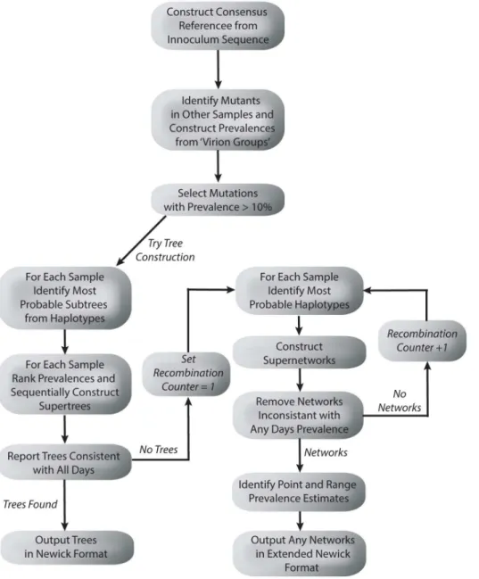
Here we provide a brief outline of our general approach, which is explained in more detail in subsequent sections. The aim of our approach was twofold. Firstly, identify mutations arising in an infection chain of viral hosts. Secondly, provide a phylogenetic tree or recombination net-work that best explains the evolution structure of the most prevalent mutations. A flow chart of the process is provided inFig 1.

Fig 1. A flow chart describing the tree and network construction process.

The first step was to sequence a time series of virus samples. Next, we took the initial sample in the time series (such as an inoculum, for example) and obtained the nucleotide with highest prevalence at each position. This defined a reference (concensus) sequence, which was then compared to the remaining samples enabling the identification of de novo mutations. The pro-portion of reads containing each mutation then represented its prevalence in the viral popula-tion (paired reads with identical start posipopula-tions, end posipopula-tions and sequences were counted once in this process, being assumed to derive from a single PCR product). Mutations with a prevalence above a (user defined) threshold (10%) on at least one sample were included for fur-ther analysis. Next we attempted to construct an evolutionary tree consistent with the preva-lence information and paired end linkage information across all samples. If no consistent tree could be identified, we attempted to construct a recombination network with one reticulation event. If this failed we iteratively increase the number of reticulation events permissable to find a recombination network consistent with the data. Any solutions obtained were outputted in either the Newick format (for trees) or the extended Newick format (for networks).

Our method used two main sources of information. Firstly, a pigeon hole principle was uti-lized, restricting how different sub-populations of viruses, each containing a certain combina-tion of mutacombina-tions, can fit within a tree or network structure. Secondly, linkage informacombina-tion was harnessed, describing how pairs of mutations co-exist in sub-populations. This information is obtained from single paired-end reads (likely to derive from a single viral particle) that con-tained two (or more) mutations.

The pigeon hole principle worked best with a set of mutation prevalences that vary signifi-cantly across the samples collected. More specifically, a subset of mutations undergoing either rapid selection or drift were found to provide the most informative datasets (RNA viruses undergoing drug treatments, or the bottleneck arising when a small number of viral particles infects an animal are examples of where this might happen). Mutations that have consistently low or high prevalence contain information that is harder to leverage, and the underlying evo-lutionary structures are harder to infer. Such mutations were not included in the analysis. Slowly mutating viruses (DNA viruses for example) are also less likely to be sufficient muta-genic for our approach.

The linkage information worked best when recombination events were relatively rare. Viruses with high rates of recombination (such as HIV) will rapidly lose linkage information making the evolutionary structure harder to identify.

We next outline the tree and network construction methods in more detail.

An Evolutionary Tree

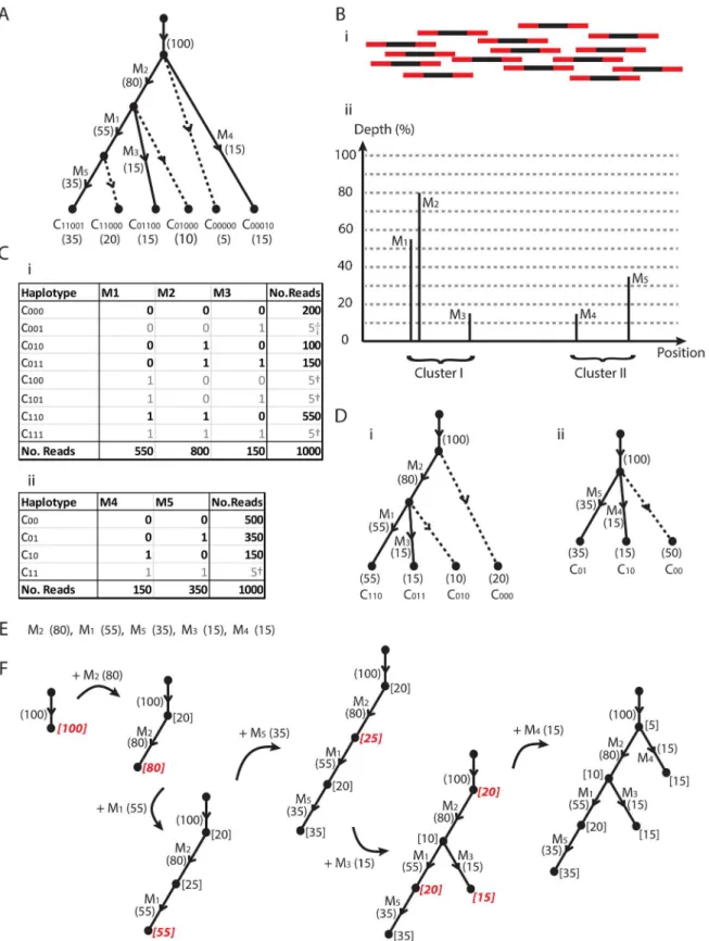
Consider the pedagogic simulation inFig 2, where we have a region of interest (such as an influ-enza segment, for example) that has undergone mutational and selective processes encapsulated by the evolution tree inFig 2A. This tree contains five mutationsM1,M2,M3,M4,M5that lie on

various branches of the tree. These combine into the six clones that are the leaves of the tree. For example, the second leaf is labeledC11000, indicating a clone with haplotype consisting of

muta-tionsM1,M2but notM3,M4,M5. Note that the path from the root of the tree to this leaf crosses

the two branches corresponding to mutationsM1andM2. The number 20 at the leaf indicates

that this clone makes up 20% of the viral population, and is termed theprevalence.

Note that these prevalences form aconserved flow networkthrough the tree [23]. For exam-ple, the prevalence of mutationM1is 55%, which accounts for the two haplotypesC11001and

C11000, with prevalences 35% and 20%, respectively. In general, we find that the prevalence

Fig 2. A super-tree sample.(A) A contrived evolution of a mixed viral population involving five mutations and six clones. Dotted lines indicate internal nodes extended to a leaf. (B) A notional representation of sequencing across the region of interest, and the resulting Depth-Position graph. Paired reads bridge two clusters of mutations. (C) Read count data obtained for the two clusters, with total depth x1000, along with artifacts†. (D) Evolutionary trees corresponding to (Ci,ii). (E) Ordered list of mutations and population prevalences (%). (F) Reconstruction of original tree in (A).

In reality we are not privy to this information and perform a sequencing experiment to investigate the structure. This takes the form of molecular sequencing, where we detect the five mutations, which each have a differentdepthof sequencing, as portrayed inFig 2B. We will later see with real influenza data that percentage depth can be reasonably interpreted as preva-lence. Furthermore, we can group mutations arising on individual sequencing reads into clus-ters. For our example, mutationsM1,M2andM3are positioned such that there are paired end

reads (exemplified inFig 2Bi) whereM1andM2will lie on the sequence at one end, andM3in

the sequence at the other end of the read. MutationsM1,M2andM3thus form one cluster.

Similarly, mutationsM4andM5can be found at the two ends of paired reads and form a

dis-tinct cluster. We then find the mutations are grouped into two clusters, giving the two corre-sponding haplotype tables inFig 2C.

We first construct an evolution tree for each of these tables. Our approach is based upon two sources of information; one utilizes mutation sequencing depth with a pigeon hole princi-ple, the other utilizes linkage information from haplotype tables.

Now we have mutationM2present in 80% of viruses and mutationM1present in 55% of

viruses. If these mutations are not both simultaneously present in a sub population of viruses, then the mutations are exclusive. This implies the two populations of size 80% and 55% do not overlap. However, the total population of viruses containing either of these viruses would then be greater than 100%<80% + 55%. This is not possible, and the only explanation is that a sub-population of viruses contain both mutations; the pigeon hole principle. The only tree-like evo-lutionary structure possible is thatM1is a descendant ofM2, as indicated by the rooted,

directed tree inFig 2Di. Note that we have not utilized any haplotype information to infer this, just the mutation prevalence of the two mutations and a pigeon hole principle.

MutationM3has a prevalence that is too low to repeat a prevalence based argument.

How-ever, we have a second source of information; the paired read data that can link together muta-tions into the haplotypes inFig 2Ci. This table is based on three mutations, which group into 23= 8 possible haplotypes. However, a tree structure with three mutations will only contain four leaves [24] and we see that four of the halpotypes (emboldened) have notably larger counts of reads and are likely to be genuine. The four haplotypes with a notably lower read counts are likely to be the result of sequencing error at the mutant base positions, or template switching from a cycle of rtPCR, and are ignored. The presence of genuine haplotypesC011andC010, lead

us to conclude thatM3is descendant fromM2but notM1, resulting in the tree ofFig 2Di.

From the mutation prevalences 55%, 80% and 15% ofM1,M2andM3, we can also use the

conserved network flow to measure the haplotypes prevalence. For example, the leaf descend-ing fromM2(80%), but notM1(55%) orM3(15%) (cloneC010ofFig 2Di) must represent the

remaining 10% = 80%−55%−15% of the population.

This provides us with two sources of information (sequencing depth and linkage informa-tion) we can utilize to reconstruct the clone haplotypes, prevalence, and evolution. However, not all mutations can be connected by sequencing reads. They may be either separated by a dis-tance beyond the library insert size, or may lie on distinct (unlinked) segments. Our approach is then as follows. We first construct a tree for each cluster of linked mutations. This will be a sub-tree of the full evolutionary structure. We then construct a supersub-tree from this set of subsub-trees.

place an edge corresponding toM2, the mutation with maximum prevalence of 80%. The next

mutation in the tree either descends from the root or this new node. Any descendants ofM2

must have a prevalence less than this 80%. Any other branches must descend from the top node but can only account for up to 20% of the remaining population. These two values are the

capacitiesindicated in square brackets. The next value we place isM1with prevalence 55%.

This is beyond the capacity 20% of the top node, soM1is descendant toM2, accounting for

55% of the 80%, leaving 25%. We thus have a three node tree with capacities 20%, 25% and 55%. The third ordered mutationM5has prevalence 35%, which can only be placed at the

bot-tom node with maximum capacity. Our next mutationM3has a prevalence 15% that is less

than any of the four capacities available, and no useful information on the supertree structure is obtained. This branch is the first to use haplotype information. We know from the first sub-tree that the corresponding branch is a descendant ofM2and notM1. The only node we can

use (in red) has capacity 25% and we place the branch. For the final branch corresponding to mutationM4, the prevalence 15% is less than four available capacities. The second subtree tells

us thatM4is not a descendant ofM5. This only rules out one of the four choices, and any of the

three (red) nodes will result in a tree consistent with the data. The top node selected results in a tree equivalent to that inFig 2A. To see this tree equivalence, the internal nodes in the last tree ofFig 2Fhave additional leaves attached (dotted lines) to obtainFig 2A.

We thus find that a single dataset can result in several trees that are consistent with the data. However, having a time series of samples means a tree consistent with all days of data is required, which will substantially reduces the solution space. Note that the prevalences of the clones at the leaves of the tree results from this recursive process. We thus find that supertree construction is relatively straightforward with the aid of prevalence.

However, trees do not always fit the data. This can be due to recombination occurring within segments, or re-assortment occurring between segments. In the next section we struct recombination networks to cater for this, although we will see that they cannot be con-structed as efficiently as trees.

A Recombination Network

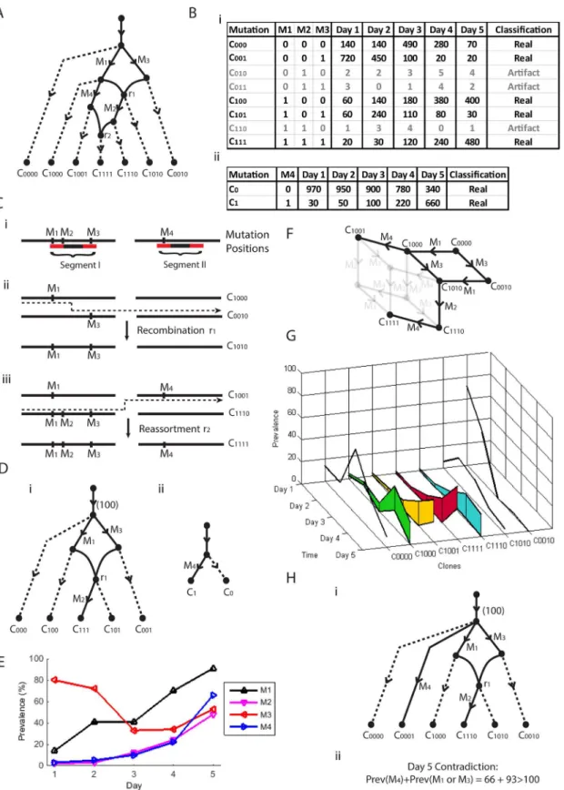
InFig 3Awe see another simulated evolution based upon the two segments inFig 3Cithat accu-mulate four mutations,M1,M2,M3 andM4. First we have mutationsM1 andM3. Then we have the first of two recombination events,r1, where we have recombination within the first seg-ment as described inFig 3Cii. We then have mutationsM2 andM4, followed by the second recombination eventr2 inFig 3Ciii, a re-assortment between the two segments. This results in the seven clones given at the leaves ofFig 3A. The prevalences of the four mutations across five time points are given inFig 3E. Note that we no longer have the conservation of prevalence observed in trees. For example, mutationsM1 andM3 are on distinct branches extending from the root, yet their total prevalence is in excess of 100% (on Day 5 for example). This is due to recombinationr1 resulting in the presence of a clone containing both mutations. The use of the prevalence to reconstruct this structure from observable data thus requires more care.

Now we see inFig 3Cithat the four mutations cluster into two groups of mutations each bridged by a set of paired reads, resulting in two tables of read counts inFig 3Bi and 3Bii. We would like to reconstruct the evolution inFig 3Afrom these data.

Fig 3. A super-network sample.(A) A pedagogic evolution recombination network with four mutations and two recombination events across two segments. (B) Typical haplotype tables arising from (A). (Ci) Two clusters of mutations grouped by paired reads on two segments. (Cii) ClonesC1000andC0010undergo within segment recombination intoC1010, with a crossover site betweenM1andM3. (Ciii) ClonesC1001andC1110undergo between segment recombination (reassortment) intoC1111. (D) Recombination networks arising from the haplotype tables in (B). (E) The prevalence of the four mutations across five days. (F) Phylogenetic network associated with (A). (G) Point and range prevalence estimates. (Hi) A network consistent with the two networks of (D). (Hii)

Incompatible prevalence conditions associated with (Hi).

way of doing this (such as ordering by prevalence which works so well with trees) so a brute force approach is taken, where we construct all possible networks that contain four mutations and the haplotypes observed inFig 3Bi and 3Bii.

This results in many candidate super-networks. We now find that the prevalence informa-tion can be used to reject many cases. For example, the super-network inFig 3Hicontains both sub-networks ofFig 3Di and 3Diias subgraphs. Note that the root node, representing the entire 100% of the population, has daughter branches containing mutationsM4,M1 andM3. How-ever, from the prevalences on Day 5 we see thatM4 has prevalence 66% andM1 andM3 (which recombine) have a collective prevalence (from clonesC001,C100,C101, andC111inFig

3Bi) of 93%. This is in excess of the possible 100% available and the network is rejected. Application of filtering by prevalence (seeMethodssection for full details) rejects all net-works with one recombination event, so we try all netnet-works with two recombination events, resulting in just seven possible recombination networks. These all contain the same set of clones, all of which correspond to the single phylogenetic network inFig 3F. Although only one recombination event is present across the subnetworks, all super-networks with one recombination event were filtered out and two recombination events were required.

Lastly we require estimates of the prevalences of each of the seven clones. We would like to match these to the prevalences in the tables ofFig 3B. This is a linear programming problem, the full details of which are given in the Methods section. The resulting estimates are given in Fig 3Gwhere we see that some clones have point estimates, whereas others have ranges. For example, we see that cloneC0010has a point estimate for each day. This is because it is the only

clone of the super-network that corresponds to cloneC001ofFig 3Biand their prevalences can

be matched. Conversely, we see ranges for the prevalences of clonesC1110andC1111. This is

because both clones correspond to cloneC111ofFig 3Biand prevalence estimates for each

clone cannot be uniquely specified.

Full details of this approach can be found in the Methods section. In the next section we describe the results obtained when applying these methods to a time series of influenza samples.

Application to Influenza

The data used in this study were generated from a chain of horse infections with influenza A H3N8 virus (sample processing details can be found in the methods section). An inoculum was used to infect two horses labeled 2761 and 6652. These two animals then infected horses labeled 6292 and 9476. This latter pair then infected 1420 and 6273. The chain continued and daily samples were collected from the horses resulting in 50 samples in total. For the present study we used 16 samples; the inoculum and hosts 2761 (days 2 to 6), 6652 (days 2, 3 and 5), 6292 (days 3 to 6) and 1420 (days 3, 5 and 6).

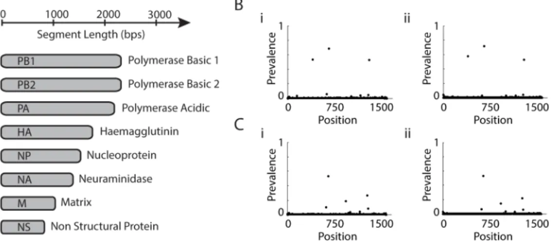
Influenza A virus is a member of the family Orthomyxoviridae which contains eight seg-mented, negative-stranded genomic RNAs commonly referred to as segments and numbered by their lengths from the longest 2341 to the shortest 890 bps [21], as summarized inFig 4A.

Daily samples were collected from each host and paired end sequenced was performed with Hi-seq and Mi-seq machines. The samples sequences were aligned with Bowtie2 [26] with default parameters. We obtain for each sample a SAM file containing mapping information of all the different reads in the sample. Any mapped read whose average Phred-quality per base was less than 30 were discarded.

To produce DNA for sequencing, viral RNA was reverse-transcribed and amplified (RT-PCR). The reverse transcription step can result in the introduction of artefact mutations that in turn would be further amplified in the PCR step, resulting in different levels of amplifi-cation and mutation. This in turn is likely to introduce significant differences between the sequencing depth and prevalence. To combat this, all identical paired end reads (with equal beginning and endpoints, and identical sequences) were grouped, classified as a single PCR product, deriving from a single molecule and only counted once.

We tested this assumption by using the observed insert size distribution to randomly simu-late reads with a number equal to the observed depth (*1.8e6 reads), assuming a single

muta-tion with prevalence of 50% exists, to determine how often two distinct events would produce identical reads. This produced a surprisingly high figure of 7% which will get worse as the depth of sequencing increases and some care is needed (see [27] for further discussion on these kind of ‘birthday paradoxes’). However, many reads contain more than one mutation making identical sequences less likely and the real figure will be somewhat lower. The depth of sequencing with these adjusted counts should then provide an improved measurement of the prevalence of viral subpopulations. We compared an identical sample that was sequenced separately (following the RT-PCR step), the results of which can be seen across two samples inFig 4Bi, 4Bii, 4Ci and 4Cii. Both the position and prevalence of mutations were reproducible to good accuracy suggesting proportional sequencing depth is a good surrogate for prevalence. We note that although there was variation in the depth of sequencing across the genome, the expected proportion of reads containing any given mutation will not change, and the depth of sequencing will not be a large source of bias on the estimated prevalence. However, we cannot rule out the possibility that some mutations are preferentially amplified, which would cause some systematic bias. We thus make the cautionary observation that some biases may exist in the prevalence, and that spike-in experiments to systematically examine the strength of correlation between sequence depth and viral prevalence are needed. Such experiments are beyond the scope of the present study and proportional sequence depth was taken as a suitable proxy for proportional viral prevalence.

We then applied the methods to sets of high prevalence mutations in each of the eight seg-ments individually, and also to a set of three mutations from distinct segseg-ments. The main observations are below.

Fig 4. Flu segments.(A) Size and function of the eight flu segments. (B,C) Depth of mutations from segment 4 from host 2761 Day 4 and host 6292 Day 3, respectively. (i,ii) Results from Hi-Seq and Mi-Seq experiments on separate libraries from the same samples.

Within Segment Evolution

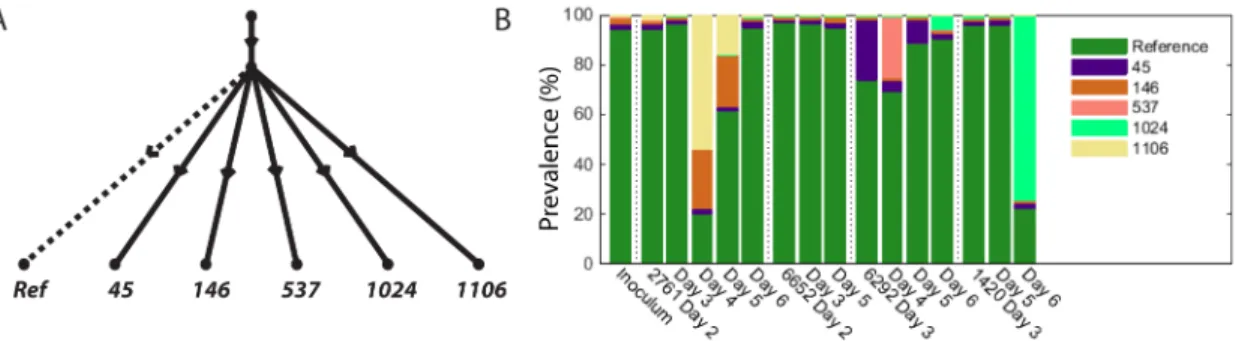
For segments 1, 3, 5, 6, 7 and 8 we obtained tree like evolutions for the segments. In all cases the mutations involved lay on distinct branches and were indicative of mutations arising in independent clones. Segment 6 can be seen inFig 5A, where we see five mutations on six branches. We also see from the stacked bar chart inFig 5Bthat many of the mutations arose during different periods in the infection chain.

However, the evolution structure of mutations within segments did not always appear to be tree like, with segment 2 containing one putative recombination event and seven mutations, and segment 4 containing three putative recombination events and six mutations. This latter case arose because we found three pairs of mutations in putative recombination. Using nucleo-tide positions as labels, these were (431, 674), (431, 709) and (709, 1401). That is, we found sig-nificant counts of all four combinations of mutations, labeledC00,C01,C10andC11, lying on

paired reads. Examples of typical counts for three (out of sixteen) samples are given in the top table inFig 6B(see Supplementary Information for full details). If the evolution is tree-like, reads from one of the typesC01,C10orC11should only arise as an artifact. Note that we have

high read counts of all four categories, which is indicative of recombination.

However, various studies have shown that there is very little evidence of genuine recombina-tion that occurs within segments of influenza [28–30], and these kind of observations can arise from template switching across different copies of segments during the rtPCR sequencing cycle [31]. We developed an analytic approach to consider this possibility in more detail.

Now if the true underlying structure is tree-like, it suggests that one ofC11,C01orC10arises

purely from template switching (the wild typeC00is assumed to always occur). This gives us

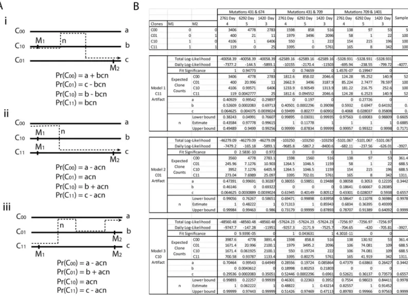
the three models (labeled i-iii inFig 6A and 6B) to consider (see also Template Switching sub-section in Methods sub-section). We leta,bandcbe the population proportions of the three real genotypes. We letnbe the probability that a cycle of rtPCR causes template switching. We then treat template switching as a continuous time three state random process. This allows us to derive probabilities that genotypesC00,C01,C10andC11arise on paired end reads, as given

inFig 6A(seeMethodsfor derivations). The counts of the four classes of read then follow a corresponding multinomial distribution. Maximum likelihood was used to estimate parame-ters, obtain log-likelihood scores, and a chi-squared measure of fit was obtained for each of the three models.

For the pair (431, 674) we found that the best log-likelihood, on all sixteen sampled days, was Model 1 (Fig 6i), where reads of typeC11are artifacts arising from template switching

alone. The parameters obtained provided an almost perfect fit; the expected counts were almost equal to the observed counts and the goodness of fit significance values were close to 1. Models Fig 5. (A) Evolution tree arising from five mutations on segment 6. (B) Prevalences of the clones across the times series.

2 and 3 (Fig 6ii and 6iii) had substantially lower likelihoods and significantly bad fits. This tells us that if the underlying structure is a tree, it involves the three genotypesC00,C01andC10and

mutations 431 and 674 lie on distinct branches.

For the pair (431, 709) we found that the best log-likelihood, over the sixteen sampled days, was Model 3 (Fig 6iii), where reads of typeC10are artifacts. The parameters obtained provided

an almost perfect fit on most days with goodness of fit significance values close to 1. A couple of days had relatively poor fits, but were not significant when multiple testing across all sixteen days was considered. Model 1 (withC11as an artifact,Fig 6i) had very similar likelihoods, but

the data exhibited significantly poor fits on multiple days. Model 2 (withC01as an artifact,Fig

6ii) performed very badly. This tells us that if the underlying structure is a tree, it involves the three genotypesC00,C01andC11and mutation 431 is a descendant of 709.

For the pair (709, 1401) we found that the best log-likelihood, on all sixteen sampled days, was Model 2 (Fig 6ii), where reads of typeC01are artifacts. The parameters obtained provided

an almost perfect fit on all days with goodness of fit significance values close to 1. Models 1 and Fig 6. (A) Three template switching models. (B) Fitted models for three pairs of linked mutations on segment 4.

3 (Fig 6i and 6iii) performed very badly. This tells us that if the underlying structure is a tree, it involves the three genotypesC00,C10andC11and mutation 1401 is a descendant of 709.

Thus the three cases where data are indicative of recombination can be explained purely by template switching during rtPCR. This is reinforced somewhat by the fact that the same model emerged across all sampled days for each mutation pair. However, this does not definitively rule out recombination, which could also exhibit these consistent patterns across sampled days, and so care is needed when interpreting data. Furthermore, the rates of template switch-ing required to explain the data without recombination were not always consistent. For exam-ple, in the sample from host 2761 Day 4, the estimated template switching between mutations (431,674) was 43.6% (95% c.i 38.2%—49.2%). Between mutations (431,709) it was 48.8% (95% c.i 46.3%—51.4%), giving reasonable agreement. Between mutations (709, 1401) it was some-what higher, at 58.6% (95% c.i 68.3%—78.7%), although this may be expected due to the greater distance between the mutations. However, in sample 1420 Day 3, the template switch-ing rate for the pair (431,674), at 99.6% (95% c.i 76.6%—99.3%), was notably higher than both the mutation pair (431,709), at 43.2% (95% c.i 39.5%—47.1%), and mutation pair (709,1401), at 49.3% (95% c.i 36.9%—64.1%). Although differences between samples (and so library prepa-rations) may be expected, differences such as this in the same library are harder to explain without implicating genuine recombination.

We thus have two explanations of the data; genuine recombination or template switching artifacts. We consider both cases and then draw comparisons.

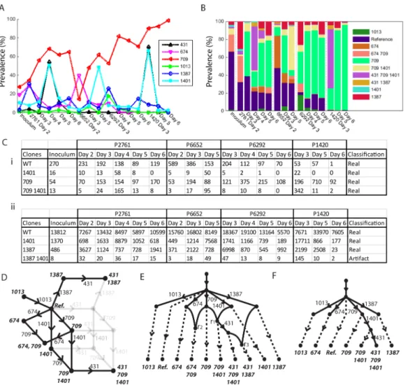
Firstly we consider segment 4 assuming recombination has taken place. The results can be seen inFig 7. The prevalences of six mutations of interest are given inFig 7A. Reasonable link-age information was available across the segment, including the two haplotype tables inFig 7C. The first is linkage information between mutations 709 and 1401, where all four combinations of mutation occur to reasonable depth, implying recombination between the mutations. The second is between mutations 1387 and 1401, where we see only three haplotypes occur to sig-nificant depth, suggesting a tree like evolutionary structure between the two mutations. The full set of tables is in Supplementary Information. Although the sequencing depth in the first table is lower, due to the rarer occurrence of sufficiently large insert sizes, the information gleaned is just as crucial. The most parsimonious evolution found involved three recombina-tion events, resulting in the single cloneset contained in the phylogenetic network given inFig 7D. There were 22 possible recombination networks that fit this phylogenetic network, one example of which is given inFig 7E. The relatively complete linkage information resulted in point estimates for the clone prevalences (rather than ranges), as given inFig 7B.

Detecting Reassortment

Re-assortments occur when progeny segments from distinct viral parents are partnered into the same viral particle, resulting in a recombinant evolutionary network.

Now re-assortment is a form of recombination. This is usually possible to detect in diploid species such as human because linkage information is available across a region of interest, such as a chromosome, and recombination can be inferred. Furthermore human samples have tinct sequencing samples for each member of the species. Inferring re-assortment across dis-tinct viral samples is more difficult because firstly we do not have linkage information across distinct segments, and secondly, we have mixed populations within each sample.

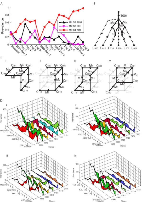
However, we show that re-assortment can still be detected within mixed population viral samples with the aid of information provided by prevalence. ConsiderFig 8. We have three mutations in segments 2, 3 and 4, along with their mutation nucleotide positions 2037, 201 and 709, respectively. We refer to the mutations asS2_2037,S3_201 andS4_709 accordingly. We see inFig 8AthatS2_2037 andS3_201 have prevalences that alternate in magnitude across the 16 days sampled. If we assume a tree like structure, these two mutations cannot lie Fig 7. (A) Mutation prevalences of six mutations in segment 4. (B) Prevalences of the ten associated clones. (C) Two tables of linked mutations exhibiting network like relationship of mutations 709 and 1401, and tree like relationship of 1387 and 1401. (D) The phylogenetic network of the single fitted cloneset. (E) One of 22 possible recombination networks that arise from (D). (F) Probable tree structure from (E) after template switching is considered.

on a single branch, because one prevalence would have to be consistently lower than the other; they must therefore lie on distinct branches. Now mutationS4_709 can; i) be on a dis-tinct third branch, ii) be a descendant ofS2_2037, iii) be a descendant ofS3_201, iv) be an ancestor ofS2_2037, v) be an ancestor ofS3_201, or vi) be an ancestor of both. We can rule out all of these choices as follows.

Firstly we note thatS4_709 has a prevalence that is consistently larger than that ofS2_2037 orS3_201, so cannot be a descendant of either mutation, ruling out ii) and iii). We see from sample 6292 Day 3 thatS2_2037 andS3_201 have a total prevalence greater thanS4_709, meaningS4_709 cannot be an ancestor of both mutations, ruling out vi). In this sample, the total prevalence of all three mutations is in excess of 100%, ruling out i). Now ifS4_709 and

S2_2037 lie on distinct branches, we see from 2761 Day 4 that their combined prevalence is in excess of 100%, ruling out v). Finally, ifS4_709 andS3_201 lie on distinct branches, we see from 6292 Day 4 that their combined prevalence is in excess of 100%, ruling out iv). No tree structure is possible and we conclude the presence of re-assortment as the most likely explanation.

In fact, application of the full method reveals that two re-assortment events are required to explain the data. This results in 51 possible recombination networks, one such example is given inFig 8B. These correspond to the four clonesets given inFig 8C, arising from two possible phylogentic networks. The four clonesets have prevalences that could not be uniquely resolved; their possible ranges are shown inFig 8D. Although we cannot uniquely identify the network or the prevalences, all solutions involved two re-assortments, one involving mutationsS4_709 andS2_2037, the other involvingS4_709 andS3_201. This observation was only possible because of inferences made with the prevalence.

Discussion

We have introduced a methodology to analyze time series viral sequencing data. This has three aims; to identify the presence of clones in mixed viral populations, to quantify the relative pop-ulation sizes of the clones, and to describe underlying evolutionary structures, including reticu-lated evolution.

We have demonstrated the applicability of these methods with paired end sequencing from a chain of infections of the H3N8 influenza virus. Although we could identify underlying evo-lutionary structures, some properties of the viruses and the resulting data make interpretation difficult. In particular, template switching during the rtPCR cycle of sequencing an RNA virus is known to occur, and can result in paired reads that imply the presence of recombination. Although any underlying tree like evolutions can still be detected, these artifacts confound the signal of any genuine recombination that may be taking place, making it harder to identify. The prevalence of mutations, measured as sequencing depth proportion, offers an alternative source of information that can help resolve these conflicts in theory, although more work is needed to evaluate how robust this metric is in practice.

Fig 8. Three mutations between three segments that indicate two re-assortment events.(A) Mutation prevalences across time series. (B) One of 51 recombination networks that fit the data. (C) Two phylogenetic networks that fit the data ((i) and (ii)-(iv)), corresponding to four clonesets. (D) Prevalence ranges for the four clonesets.

mutations, for example. The application of prevalence thus needs to be used with caution, and further studies are needed to fine tune this type of approach.

When the approach was applied to mutations in distinct segments, two re-assortment events were inferred. The differences in mutation prevalences were more marked in this case suggesting the inference is more robust and re-assortment more likely to have taken place. This is also biologically more plausible, with events such as this accounting for the emergence of new strains. We note that although re-assortment may have genuinely taken place, only one of the original clones (containing just mutation 709 on segment 4) survived the infection chain and a longitudinal study would not have picked up such transient clonal activity.

These methods utilized paired end sequencing data and showed that even when paired reads do not extend the full length of segments, or bridge distinct segments, we can still make useful inferences on the underlying evolutionary structures. The two main sources of informa-tion are the linkage offered by two or more mutainforma-tions lying on the same paired reads, and the prevalence information. We note, firstly, that utilising the full range of insert sizes produced in the sequencing library provides linkage information that covered most distances across seg-ments. Filtering paired reads to remove inserts with larger insert sizes can lose useful linkage information. Indeed, it is likely to be profitable to produce libraries with different insert sizes. Secondly, we note that it is by utilizing the variability of the prevalence in a time series dataset that we can narrow down the predictions to a useful degree; application of this method to indi-viduals days will likely result in too many predictions to be useful. Furthermore, this has great-est application to mutations of higher prevalence; this places more rgreat-estrictions on possible evolutions consistent with the data. Subsequently, this kind of variability is most likely to mani-fest itself under conditions of differing selectional forces. A stable population is less likely to contain mutations moving to fixation under selective forces. Lower prevalence mutations will result, meaning less predictive power. Simulations also suggest that although clone-sets may be uniquely identified, prediction of the underlying reticulation network is difficult, with many networks explaining the same dataset.

As we lower the minimum prevalence of analyzed mutations, their number will increase. The number of networks will likely explode and raise significant challenges. Furthermore, sin-gle strand RNA viruses such as influenza mutate quickly, suggesting a preponderance of low prevalence mutations likely exist. This is further exacerbated by the fact that sequencing uses rt-PCR, introducing point mutations and template switching artifacts that create noise in the data. These processes are likely responsible for the grass-like distribution of low prevalence mutations visible inFig 4B and 4C. Thus as we consider lower prevalence mutations we are likely to get a rapidly growing evolution structure of increasingly complex topology. The meth-ods we have introduced, however, can provide useful information at the upper-portions of these structures.

The software ViralNet is available atwww.uea.ac.uk/computing/software. The raw data is available from the NCBI (project accession number SRP044631). More detailed outputs from the algorithm are available in Supplementary Information.

Methods

We now outline details of sample preparation, tree and network construction methods, a tem-plate switching model, and method validation.

Sample Preparation

RT-PCR as described in [5] and [32] was performed. Virus copy numbers are available in sup-plementary information. Full genome amplification was performed as described in [33]. Each DNA sample was then processed for paired end sequencing on both a Hi-Seq and Mi-Seq machine, producing ends with 101 bases.

The reads from the innoculum sample were then used to construct a majority reference sequence. Reads from samples further down the infection chain were compared against this reference for variant calling. Paired reads with identical start and end reference points, and identical sequences, were deemed to arise from a single PCR product. Duplicates were thus removed and only one paired read is selected for the final dataset.

Tree Construction

The construction of phylogenetic trees is a well established area [24]. Trees are frequently con-structed from tables of haplotypes of different species. However, we have two properties that change the situation. Firstly, if we have a set ofnmutations linked by reads, we can have up to 2ndistinct haplotypes. However, a consistent set of splits from such a table should only have up ton+ 1 distinct haplotypes, in a split-compatible configuration [24]. To construct a phyloge-netic tree we thus need to classify the genotypes as real or artifact. Secondly, we have prevalence information, in the form of a conserved network flow through the tree. This can help us to both decide which haplotypes to believe and to construct a corresponding tree.

To describe the algorithm we first introduce some notation. Now, the evolutionary structure is represented by two types of rooted directed tree; one where each edge represents a mutation, such as inFig 2F, and one where all leaves represent clones in the population, such as inFig 2A and 2D. The first is a subtree of the latter. The latter has a conserved flow network. These will be termed theCompact Prevalence TreeandComplete Prevalence Treerespectively.

Now to each edgeein the compact prevalence tree, we assignprevalenceρ(e). This

repre-sents the proportion of population containing the mutation represented by the edgee. The sin-gle directed edgeein(v) pointing toward a vertexv(away from the root) represents a viral population of prevalenceρ(ein(v)), all containing the mutation corresponding to edgeein(v),

along with its predecessor mutations. The set of daughter edgesEout(v) leading away from node

vrepresent populations containing subsequent mutations, each with prevalenceρ(e),e2 Eout(v). The remaining population fromρ(ein(v)) contains just the original mutation set, having

a prevalence described by thecapacityz(v). The conservation of prevalence satisfied by each vertexv2Tis then represented by the condition:

rðeinðvÞÞ ¼zðvÞ þ X

e2EoutðvÞ

rðeðvÞÞ _ð1Þ

The root node has total prevalence of 1, representing the entire population of interest. This describes the mutation based trees such as that inFig 2F. To obtain a complete tree containing all the clones, we need to extend an edge from each internal node to represent the associated clone (these are the dashed lines inFig 2A). The prevalence of the additional edges are equal to the capacities of the parental nodes.

The algorithm is broken into two steps. The first calculates subtrees. The second calculates supertrees.

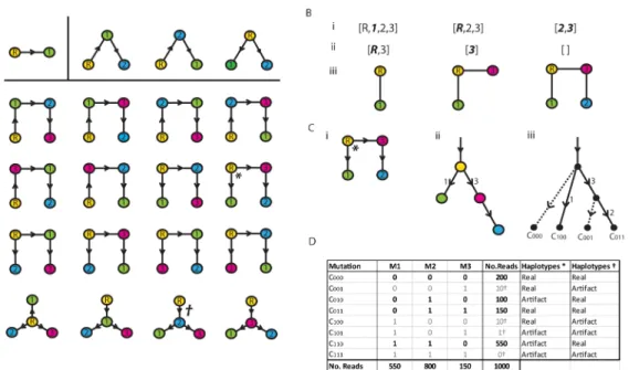
Step 1 Subtree construction. Now, fornmutations we have 2npossible haplotypes, with corresponding countsni,i= 1, 2,. . ._{, 2}n_{, and a tree withn+ 1 haplotypes to fit. This implies} that 2n−n−1 of those counts are artifacts. For example, inFig 9Dwe see the simulated counts

for 23haplotypes on 3 mutations. Now Cayley’s formula states that there arenn−2_different

labeled trees that can be constructed on n vertices [34]. These are easily constructed with the aid of Prüfer sequences [35], which are any integer sequence [p1,. . .,pn−2] such thatpi2{1, 2, . . ._{,n}. The first few examples are given inFig 9A.}

To construct a tree we start withp= [p1,. . .,pn−2] and the vectorv= [1, 2,. . .,n]. At each

step we take the lowest entry ofvnot inp, and the lowest entry ofp, and join the two corre-sponding nodes together with an edge. For example inFig 9Bwe start withv= [R, 1, 2, 3], where the root nodeRis treated as the minimum value, along with Prüfer sequencep= [R, 3]. The smallest element ofvnot inpis 1. The corresponding node is then joined to the node for the smallest elementRofp, such as exemplified inFig 9Biii. These two elements are removed frompandvand the process repeated until we are left with two elements inv. Our example leaves us with the two elements 2 and 3, the corresponding nodes of which are then joined by an edge. The edges are then directed away from the root, resulting in the prevalence clonal tree inFig 9Cii. The corresponding complete prevalence tree is inFig 9Ciii.

Once we have all the possible subtrees constructed, we use maximum likelihood to select the most plausible tree. Consider, for example, the penultimate column ofFig 9D, which corre-spond to the four haplotypes for the tree () inFig 9A–9C. Note that the haplotypeC110with a

count 550 is an artifact for this tree. If each mutation artifact arises with probability, then an artifact read of typeC110contains two mutant bases and occurs with probability2. We can

then construct log-likelihoods (summed across time points) for the artifact counts arising from clones that do not belong to the putative tree being tested. We then assume Poisson distributed Fig 9. (A) Cayley trees for 2, 3 and 4 vertices. (Bi) Vertex listvfor example (*). (Bii) Prüfer sequencep. (Biii) Tree construction. (Ci) The graph directed away from the root. (ii) The equivalent compact clonal tree. (iii) The corresponding complete clonal tree. (D) Alignment of trees*and†to haplotype tables.

counts and construct the following likelihood function for a given putative clonal treeT_:

L_ðT_{Þ ¼}X t

X

h2=T

logðPoiss_nðtÞ

j

ðnðtÞxðhÞ_ÞÞ

ð2Þ

Heretindexes the time point,n(t)and= 0.003 are the total depth and the error rate, respectively. The valuesx(h) represents the number of mutants in haplotypeh. The tree with maximum likelihood is selected. Although the use of a Poisson distribution may be approxi-mate, this technique is a pragmatic way to identify plausible haplotypes/trees.

Step 2 Supertree construction. We next build supertrees of the evolution from the sub-trees. As we saw in the example inFig 2F, this involves ranking the subtree branches by preva-lence, and adding mutations sequentially as in the example inFig 2F, checking pairwise ancestry relationships between mutations (from the subtrees), along with the capacity of preva-lence available at each node (by checkingEq (1)for every time point).

Note that this algorithm may produce no trees. This implies there are no supertrees consis-tent with the data, and recombination networks may be more suitable.

The Recombination Algorithm

We would like to use data such asFig 3Bto reconstruct the evolutionary structure. The splits method [25] is used to construct phylogenetic networks such asFig 3G. There are many recom-bination networks that correspond to any given phylogenetic network. A standard method to identify recombination networks is to look for an optimal path of trees across the recombina-tion sites [36]. These methods generally have the full mutarecombina-tion profile of a set of species of interest to compare. Our problem is exacerbated by missing data and the full haplotypes of dis-tinct species (clones in our case) are not available. However, we have prevalence information which can help identify structures consistent with the data.

We construct recombination networks in five steps; haplotype classification, super-network construction, super-network filtering, prevalence maximum likelihood estimation, and preva-lence range estimation. We describe these steps in detail.

Step 1 Haplotype classification. In order to distinguish the real and artifact haplotypes in any table such asFig 7Cwe do the following. For any countnðtÞh associated with haplotypeh

and time pointt, we calculate the probability it arises as an error using the Poisson distribution. This gives a term of the formPoiss_nðtÞ

h

ðnðtÞxðhÞ_{Þ, wheren}(t)_{is the total read depth from that time}

point,x(h) is the number of mutations distinct from the wild type, andis a user selected error rate per base per read. We then take the combined log-likelihoodL_{across all time points. All}

log-likelihoods below a thresholdL_{0are classified as real. The values= 0.003 and}L_{0 ¼} 350 were used in implementation. An error rate of= 0.003 is a conservative overestimate of the true error rate [37]. The likelihood threshold was the value that misclassified the least number (4%) of haplotypes (where‘real’haplotypes were defined to be those containing at least one prevalence above 10%). This threshold can be lowered if the inclusion of lower prevalence hap-lotypes is desirable, although more false positive haphap-lotypes will subsequently be included.

Step 2 Super-network construction. This is a brute force approach where we construct all possible recombination networks usingr= 0, 1, 2,. . ._{reticulated nodes in turn. Any networks} that do not contain the real haplotypes of the individual haplotype tables of Step 1 are rejected. The value ofrselected is the smallest value with any valid networks after Steps 3 and 4 are implemented.

population. We letρcdenote the prevalences of that clone. We then have the conditions:

X

c

r_c¼1_;r

c0 ð3Þ

Now we have the estimated prevalenceλ_{mof each mutationm= 1, 2,}. . ._{,Mfrom the} pro-portional sequencing depth at the mutations position. If we letCmdenote the set of clones

from the super-network that contain mutationm, we have conditions of the form:

X

fc2C_mg

r_c¼l_{m ð4Þ}

We solve the linear programming problem defined by Eqs3and4with the simplex method. If no solution exists on any daytthe network is rejected. If a solution is found, it is the input to the (more precise) calculation in Step 4. This step generally reduces the number of networks to manageable levels.

Step 4 Prevalence point estimation. In realityλ

mis an estimate and we have more

infor-mation than just the depth of mutations. For each cluster of mutations we have the countnðtÞh

for each real genotypeh(artifacts are ignored) and time pointstin the corresponding table. Conditioning on the total countn(t)of real genotypes results in a binomial log-likelihood of the following form:

L_¼X h

nðtÞh logðn ðtÞX

c2Ch

rðtÞ c Þ

Here the sum is over the setChof clones that contain haplotypeh. We then sum this over all tables and time points and maximize for estimates of the clone prevalencesrðtÞ

c . We use

gradi-ent descgradi-ent to maximize, projecting each step onto the simplex inEq 3. Projecting onto the simplex is relatively straightforward, the updated prevalence vectorρjust becomes_jjrjjr₁, where

negative components are set to zero.

Step 5 Range estimation. Step 4 does not always result in a unique estimate, because there may be ranges of valuesrðtÞ

c on the simplex ofEq 3that yield identical terms P

c2s rðtÞ

c . Then ifr^ ðtÞ c

are the estimates from the gradient descent, we use the simplex method to maximizerðtÞ c

sub-ject toEq 3and conditions of the form:

X c2s rðtÞ c ¼ X c2s ^ rðtÞ c

Valid clonesets with the maximum likelihood are then selected. This can be applied to any putative network to either conclude that the network is not feasible, or produce a range of pos-sible prevalences associated with the network.

Template Switching

We model template switching during rtPCR as follows. Suppose we have two mutations of interest and four possible genotypes, labeledC00,C01,C10andC11. We have corresponding

read depth countsn00,n01,n10andn11. Now, if tree like evolution exists, one ofC01,C10orC11

is an artifact arising from template switching during rtPCR (the wild type C00 is assumed to always occur). We demonstrate the case whereC01is an artifact (model 2 inFig 6Aii). The

deri-vation for the other two models is similar. Then we assume that the real clonesC00,C10andC11

We model rtPCR as a time continuous three state process, where template switching occurs at a rateλ_{, jumping to any of the three templatesC}

00,C10orC11with probabilitiesa,bandc,

respectively. We also refer to the states asa,bandc. The template switching rateλ_{is taken to}

be a constant, which is equivalent to assuming template switching occurs with uniform proba-bility along the segments. Any sequence context effects along segments are ignored. We let

pa(t),pb(t) andpc(t) be the probabilities of occupying a copy of the corresponding templates at positiont. Then conditioningpa(t) over a time interval (t,t+dt) results in the following expres-sion (see [38] for typical derivations):

p_aðtþdtÞ ¼p_aðtÞð1 _{ldtÞ þp}

aðtÞaldtþpbðtÞaldtþpcðtÞaldt

This gives us the following differential equation and solution:

dpa

dt ¼lða paÞ,paðtÞ ¼aþ ðpað0Þ aÞe lt

We rescale time so thatt= 1 represents one rtPCR cycle. We then have the following transi-tion matrix between states:

T¼

aþ ð1 _aÞe l _{b be} l _{c ce} l

a ae l _{bþ ð1 bÞe} l _{c ce} l

a ae l _{b be} l _{cþ ð1 cÞe} l

0 B B B @ 1 C C C A

Probabilities for all typesC00,C01,C10andC11can now be defined, which we demonstrate

forC10. Derivations for the other terms can be obtained in a similar manner. FromFig 6Aiiwe

see that to obtain a read of the formC10, we can start in either stateborcand end in either

stateaorb. This gives us four terms to add:

PrðC10Þ ¼bTbaþbTbbþcTcaþcTcb¼bða ae

l_{þbþ ð1 bÞe} l_{Þ þcða ae} l_{þb be} l_{Þ ¼bþacn}

Heren= 1−e−

λ

is the probability a template switch occurs. The formulas inFig 6Aare obtained similarly.

The countsn00,n01,n10andn11then follow a multinomial distribution, from which

log-like-lihoods can be derived. A chi-squared goodness of fit can then be obtained. We note that in many cases, solutions for the four termsPr(C00),Pr(C01),Pr(C10) andPr(C11) in terms ofa,b,c

andncan be obtained, resulting in a perfect fit. When this is not possible, one or more of the three models can be rejected if the fit is sufficiently bad.

Note that none of these three models necessarily explain the data. In the last column ofFig 6D, for example, we have four artificial counts 50, 1000, 1000 and 1000 corresponding to geno-typesC00,C01,C10andC11. All three models are a bad fit suggesting recombination is present.

However, this relies on small counts forC00, which were not observed in the real data that was

examined.

Note that template switching has no effect on the prevalence of individual mutations. For example, consideringFig 5Ciii, if we addPr(C01) andPr(C11), we getb+c, which is precisely

the prevalence of mutationM2.

Validation and Simulation

software Shorah using the same simulation approaches as Zagordi et al [12,15] and Astro-vskaya et al. [16].

To measure the performance of the mixed population estimation, we computed the Preci-sion, theRecall, and theAccuracyof prevalence estimation for the methods of interest. The recall (or sensitivity) gives the ratio TP

TPþFNof correctly reconstructed haplotypes to the total

number of true haplotypes, where we have true positives (TP), false negatives (FN) and false positives (FP). The precision gives their ratio to the total number of generated haplotypes,

TP TPþFP.

The accuracy measures the ability of the method to recover the true mixture of haplotypes, and was defined as measuring the mean absolute error of the prevalence estimate. Where a range estimate is obtained for the prevalence, we calculate the shortest distance from the true value to the range.

Comparison with Shorah was done on simulated deep sequencing data from a 1.5 kb-long region of HIV-1. Simulated reads have been generated by MetaSim [39], a meta-genomic simu-lator which generates collections of reads reproducing the error model of some given technolo-gies such as Sanger and 454 Roche. It takes as input a set of genome sequences and an

abundancy profile and generates a collection of reads sampling the inputted genomic population.

For up to 12 haplotypes and 3 reticulations we performed 100 runs as follows. We randomly constructed a network by attaching each new branch to a random selected node. Reticulations were also randomized. The prevalences of the resulting clones (at the leaves) were randomly selected from a Dirichlet distribution. This is repeated for 10 time points of data. We used MetaSim to generate a collection of 5,000 reads having an average length of 500bp and replicat-ing the error process of Roche 454 sequencreplicat-ing. The methods were then applied to the resultreplicat-ing data.

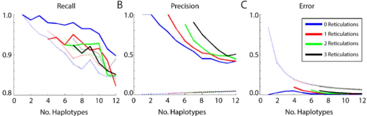
Shorah output can display mismatches or gaps in the outputted genomes, with increasing frequency at the segment edges. We applied a modification on Shorah output by trimming the edge and we then corrected one or two mismatches or gaps on all the genomes before address-ing the comparison.Fig 10A–10Cprovide the comparison for recall, precision and error indi-cators. We found slight improvements for recall, especially for tree like evolution. The precision and error also had improved results. We acknowledge that the simulations were based upon evolutionary structures that the models are designed to fit so such improvement might be expected. Furthermore, Shorah likely have better performance on low prevalence clones. However, these simulations demonstrate that reasonable results can be obtained from the techniques we have introduced.

Fig 10. Validation profiles for a range of haplotype counts, including; (A) Recall, (B) Precision, and (C) Error.In all cases the solid line denotes the algorithm preformance, the dashed line indicates Shorah performance.

Supporting Information

(CSV)

S2 Data. Hi-seq Coverage.

(CSV)

S3 Data. Mi-seq Coverage.

(CSV)

S4 Data. Output Information.

(XLSX)

S5 Data. Viral Copy Numbers.

(PDF)

S1 File. Segment 1 Networks for visualisation in Dendroscope.

(TXT)

S2 File. Segment 2 Networks for visualisation in Dendroscope.

(TXT)

S3 File. Segment 3 Networks for visualisation in Dendroscope.

(TXT)

S4 File. Segment 4 Networks for visualisation in Dendroscope.

(TXT)

S5 File. Segment 5 Networks for visualisation in Dendroscope.

(TXT)

S6 File. Segment 6 Networks for visualisation in Dendroscope.

(TXT)

S7 File. Segment 7 Networks for visualisation in Dendroscope.

(TXT)

S8 File. Segment 8 Networks for visualisation in Dendroscope.

(TXT)

S9 File. Cross Segment Networks for visualisation in Dendroscope.

(TXT)

Author Contributions

Conceived and designed the experiments: CDG PRM DFC. Performed the experiments: CDG PRM DFC. Analyzed the data: CDG PRM DFC. Contributed reagents/materials/analysis tools: CDG PRM DFC. Wrote the paper: CDG PRM DFC.

References

1. Beerenwinkel N and Zagordi O, 2011, Ultra-deep sequencing for the analysis of viral populations,Curr. Opin. Virol, 1(5), 413–418. doi:10.1016/j.coviro.2011.07.008PMID:22440844

3. Skums P, Mancuso N, Artyomenko A, Tork B, Mandoiu I, Khudyakov Y and Zelikovsky A, 2013, Recon-struction of Viral Population Structure from Next-Generation Sequencing Data Using Multicommodity Flows,BMC Bioinformatics, 14(9), S2. doi:10.1186/1471-2105-14-S9-S2PMID:23902469

4. Murcia PR, Hughes J, Battista P, Lloyd L, Baillie GJ, Ramirez-Gonzalez RH, Ormond D, Oliver K, Elton D, Mumford JA, Caccamo M, Kellam P, Grenfell BT, Holmes EC and Wood JLN, 2012, Evolution of an Eurasian Avian-like Influenza Virus in Naive and Vaccinated Pigs, 8(5), e1002730,PLOS Pathogens. doi:10.1371/journal.ppat.1002730PMID:22693449

5. Murcia PR 1, Baillie GJ, Daly J, Elton D, Jervis C, Mumford JA, Newton R, Parrish CR, Hoelzer K, Dou-gan G, Parkhill J, Lennard N, Ormond D, Moule S, Whitwham A, McCauley JW, McKinley TJ, Holmes EC, Grenfell BT, Wood JL, 2010, Intra- and interhost evolutionary dynamics of equine influenza virus,J Virol., 84(14), 6943–54. doi:10.1128/JVI.00112-10PMID:20444896

6. Zagordi O and Töpfer A and Prabhakaran S, Roth V, Halperin E and Beerenwinkel N, 2012, Probabilis-tic inference of viral quasispecies subject to recombination, Research in Computational Molecular Biol-ogy, Springer, 342–354.

7. Luciani F, Bull RA and Lloyd AR, 2012, Next generation deep sequencing and vaccine design: today and tomorrow,Trends in biotechnology, 30(9), 443–452. doi:10.1016/j.tibtech.2012.05.005PMID:

22721705

8. Prosperi MCF, Prosperi Luciano and Bruselles A, Abbate I, Rozera G, Vincenti D, Solmone MC, Capo-bianchi MR and Ulivi G, 2011, Combinatorial analysis and algorithms for quasispecies reconstruction using next-generation sequencing,BMC bioinformatics, 12(1), 5. doi:10.1186/1471-2105-12-5PMID:

21208435

9. Barzon L, Lavezzo E, Militello V, Toppo S and Palù G, 2011, Applications of next-generation sequenc-ing technologies to diagnostic virology,International journal of molecular sciences, 12(11), 7861–

7884. doi:10.3390/ijms12117861PMID:22174638

10. Pybus OG and Rambaut A, 2009, Evolutionary analysis of the dynamics of viral infectious disease, Nature Reviews Genetics, 10(8), 540–550. doi:10.1038/nrg2583PMID:19564871

11. Beerenwinkel N and Günthard HF, Roth V and Metzner KJ, 2012, Challenges and opportunities in esti-mating viral genetic diversity from next-generation sequencing data,Frontiers in Microbiology, 3, 329. doi:10.3389/fmicb.2012.00329PMID:22973268

12. Zagordi O, Geyrhofer L, Roth V and Beerenwinkel N, 2010, Deep sequencing of a genetically heteroge-neous sample: local haplotype reconstruction and read error correction,Journal of computational biol-ogy, 17(3), 417–428. doi:10.1089/cmb.2009.0164PMID:20377454

13. Eriksson N, Pachter L, Mitsuya Y, Rhee S, Wang C, Gharizadeh B, Ronaghi M, Shafer RW and Beeren-winkel N, 2008, Viral population estimation using pyrosequencing,PLoS Computational Biology, 4(5), e1000074. doi:10.1371/journal.pcbi.1000074PMID:18437230

14. Westbrooks K, Astrovskaya I, Campo D, Khudyakov Y, Berman Piotr and Zelikovsky A, 2008, HCV quasispecies assembly using network flows,Bioinformatics Research and Applications, 159–170, Springer.

15. 2011, Zagordi O, Bhattacharya A, Eriksson N and Beerenwinkel N, ShoRAH: estimating the genetic diversity of a mixed sample from next-generation sequencing data,BMC bioinformatics, 12(1), 119. doi:10.1186/1471-2105-12-119PMID:21521499

16. Astrovskaya I, Tork B, Mangul S, Westbrooks K, Măndoiu I, Balfe P and Zelikovsky A, 2011, Inferring viral quasispecies spectra from 454 pyrosequencing reads,BMC bioinformatics, 12(6), S1. doi:10. 1186/1471-2105-12-S6-S1PMID:21989211

17. O’Neil ST and Emrich SJ, 2012, Haplotype and minimum-chimerism consensus determination using short sequence data,BMC genomics, 13(2), S4. doi:10.1186/1471-2164-13-S2-S4PMID:22537299 18. Mancuso N, Tork B, Skums P Mandoiu I and Zelikovsky A, 2011, Viral quasispecies reconstruction

from amplicon 454 pyrosequencing reads,Bioinformatics and Biomedicine Workshops (BIBMW), 2011 IEEE International Conference, 94–101.

19. Huang A, Kantor R, DeLong A, Schreier L and Istrail S, 2011, QColors: An algorithm for conservative viral quasispecies reconstruction from short and non-contiguous next generation sequencing reads,In silico biology, 11(5), 193–201. PMID:23202421

20. Prabhakaran S, Rey M, Zagordi O, Beerenwinkel N and Roth V, 2010, HIV-haplotype inference using a constraint-based dirichlet process mixture model,Machine Learning in Computational Biology (MLCB) NIPS Workshop, 1–4.

21. Tsaic K and Chen G, 2011, Influenza genome diversity and evolution,Microbes and Infection, 13(5), 479–488. doi:10.1016/j.micinf.2011.01.013

H1N1/2009) by de novo sequencing using a next-generation DNA sequencer,PLoS One, 5(4), e10256. doi:10.1371/journal.pone.0010256PMID:20428231

23. Papadimitriou PH, 1982,Combinatorial Optimization, Dover.

24. Semple C and Steel M, 2003, Phylogenetics, OUP.

25. Huson D, Rupp R and Scornavacca C, 2010,Phylogenetic Networks, Concepts, Algorithms and Appli-cations, CUP.

26. Langmead B and Salzberg SL, 2012, Fast gapped-read alignment with Bowtie 2,Nature Methods, 9 (4), 357–359. doi:10.1038/nmeth.1923PMID:22388286

27. Sheward DJ, Murrell B and Williamson C, 2012, Degenerate Primer IDs and the birthday problem,Proc Natl Acad Sci U S A, 109(21), E1330. doi:10.1073/pnas.1203613109PMID:22517746

28. Boni MF, Smith GJ, Holmes EC, Vijaykrishna D, 2012, No evidence for intra-segment recombination of 2009 H1N1 influenza virus in swine,Gene, 494(2), 242–5. doi:10.1016/j.gene.2011.10.041PMID:

22226809

29. Boni MF, Zhou Y, Taubenberger JK, Holmes EC, 2008, Homologous recombination is very rare or absent in human influenza A virus,J Virol., 82(10), 4807–11. doi:10.1128/JVI.02683-07PMID:

18353939

30. Boni MF, de Jong MD, van Doorn HR, Holmes EC, 2010,PLoS One, 5(5), e10434. doi:10.1371/ journal.pone.0010434PMID:20454662

31. Simon-Loriere E and Holmes EC, 2011, Why do RNA viruses recombine?,Nature Reviews Microbiol-ogy, 9, 617–626. doi:10.1038/nrmicro2614PMID:21725337

32. Murcia PR, Baillie GJ, Stack JC, Jervis C, Elton D, Mumford JA, Daly J, Kellam P, Grenfell BT, Holmes EC and Wood JLN, 2013, Evolution of Equine Influenza Virus in Vaccinated Horses,J. Virol., 87(8), 4768–4771. doi:10.1128/JVI.03379-12PMID:23388708

33. Zhou B, Donnelly ME, Scholes DT, George K St., Hatta M, Kawaoka Y, and Wentworth DE, Single-Reaction Genomic Amplification Accelerates Sequencing and Vaccine Production for Classical and Swine Origin Human Influenza A Viruses, 2009,J. Virol., 83(19), 10309–10313. doi:10.1128/JVI. 01109-09PMID:19605485

34. Cayley A, 1889, A theorem on trees,Quart. J. Math, 23, 376–378.

35. Prüfer H, 1918, Neuer Beweis eines Satzes über Permutationen,Arch. Math. Phys., 27, 742–744.

36. Song YS and Hein J, Constructing Minimal Ancestral Recombination Graphs, 2005,J. Comp Bio., bf 12(2), 147–169. doi:10.1089/cmb.2005.12.147

37. Sanjuán R, Nebot MR, Chirico N, Mansky LM and Belshaw R, 2010, Viral mutation rates,J. Virol., 84, 9733–9748. doi:10.1128/JVI.00694-10PMID:20660197

38. Bunday BD, 1996,An Introduction to Queueing Theory, Arnold.