THE TAYLOR RULE UNDER INQUIRY: Hidden states
1
Rodrigo De Losso da Silveira Bueno
2EAESP-FGV/UNIVERSITY OF CHICAGO
September 15, 2005
1Work in progress, so comments are very welcome. I would like to express my gratitude for the
invaluable contributions of Andr´e Silva, Jos´e Resende, Marcos Mollica, Ricardo Avelino, Daniel Santos, Lars Hansen, John Cochrane, Monika Piazzesi, and the seminar participants at FGV-SP, IBMEC-RJ and EPGE for their comments. I would also like to thank CAPES for providing theirfinancial support. Any errors found in this paper are mine.
Abstract
This work empirically evaluates the Taylor rule for the US and Brazil using Markov-Switching
Regimes. I find that the inflation parameter of the US Taylor rule is less than one in many
periods, contrasting heavily with Clarida, Gal´ı and Gertler (2000), and the same happens with
Brazilian data. When the inflation parameter is greater than one, it encompasses periods that
these authors considered they should be less than one. Brazil is used for comparative purposes
because it experienced a high level inflation until 1994 and then a major stabilization plan
reduced the growth in prices to civilized levels. Thus, it is a natural laboratory to test theories
designed to work in any environment. The findings point to a theoretical gap that deserves
further investigation and show that monetary policy in Brazil has been ineffective, which is
coherent with the general attitude of population in relation to this measure.
Key Words: Markov-Switching Regimes, Hidden States, Taylor Rule
1
INTRODUCTION
Taylor (1993) describes US monetary policy using a simple linear function linking nominal
inter-est, it, to inflation,πt, and to output gap, xt. Since then, a number of authors have established
the economic fundamentals that support such an empirical finding, known as the Taylor Rule,
roughly defined as follows: it = gππt +gxxt. Taylor (1999) contains several empirical studies
regarding it, and Woodford (2003), among others, was able to derive optimal rules that are closer
versions of Taylor’s.
Clarida, Gal´ıand Gertler (2000) show that the inflation parameter of the Taylor Rule varies
with different samples. In particular, the inflation parameter is greater than one after Volcker
became chairman of the FED, and it is less than one before that event. Their results depend
crucially on their choice regarding when to break the series. They make such a break to
charac-terize a shift in the monetary policy. However, by varying the date the results may be modified,
as well as being always arbitrary due to the exogenous determination of this factor.
In this paper I use the Markov Switching Regime framework to estimate the regimes that
the monetary policy may have experienced. The procedure is appropriate because the choice of
the regimes is endogenous to the econometric model, mitigating the criticisms placed on Clarida,
Gali and Gertler. We can then check the reliability of their assumptions and estimates. It is
also interesting because one may access variations in regimes and verify how policy makers have
changed their behavior, given that the econometrician does not directly observe such changes.
We apply the same procedure for Brazil for several reasons. The first is that the
countrysuf-fered a very pronnounced latent hyperinflation period. However, in 1994 a monetary stabilization
plan, the so-called Real Plan, was launched and brought inflation down to civilized levels. This
successful plan clearly divided the regimes in Brazil and may be easily observed in figure 1.
Before the Real Plan, others were implemented, but failed, and I label them as Collor 1 and
Collor 2 in the figure. Therefore, the procedure should divide clearly both periods, and this is
indeed what happens as I demonstrate later on (see figure 5).
However, the same is not true for the US, at least not in the terms proposed by Clarida,
Gal´ı and Gertler. Therefore, I suggest that their conclusions were driven by the choice made
Figure 1: Interest x Inflation - Brazilian Monthly Data
.0 .1 .2 .3 .4 .5 .6
1990 1992 1994 1996 1998 2000 2002
INTEREST RATE INFLATION (IPCA)
Collor 1
Collor 2
Real Plan
that there were a few periods in which extreme values have influenced the inflation parameter,
forcing it above one. To support this claim, I rely on Bueno’s (2005a) data set, who finds very
similar conclusions to Clarida, Gal´ı and Gertler by using a Kalman Filter and nonlinear least
squares estimation procedures.
Notwithstanding, it is a fact that the US is a mature economy with no price indeterminacy.
Therefore it is fair to ask why I arrive at such conclusions. That gives us the second reason to
put Brazil in this paper.
After the Real Plan, inflation fell dramatically and has sincefluctuated around 7% per annum.
No one would claim that Brazil currently experiences high inflation levela or has uncontrolled
prices, which would signify price indeterminacy. However, I show in this study that even after the
Real Plan, the inflation parameter in Brazil has not increased and exceeded one (which means
theoretically price determinacy) as would expected after such a plan. This astonishing finding
supports Bueno (2005a, 2005b), which varies econometric methods, data frequency, proxies for
output and output gap and mantains these conclusions. Therefore, by contrasting Brazil with
the US, I am able to argue that there is some unexplained gap in theory which deserves more
The remainder of this work is organized as follows: Section 2 discusses the econometric Taylor
rule model that I use in the estimations; Section 3 reports the results using Markov-Switching
regimes for the US; and Section 4 applies the same model to Brazilian data. The last section
serves a conclusive point to this study.
2
THE TAYLOR RULE AND MARKOV SWITCHING
REGIMES
I follow Clarida, Gal´ı and Gertler (2000) to formulate the model. First, suppose the Central
Bank defines a target rate given by:
i∗t =i∗st +gπ,st
£
Et(πt,k)−π∗st
¤
+gx,stEt(xt,q), (1)
where
πt,k is the inflation rate in log terms between periods t and t+k;
π∗st is the target for inflation;
xt,q is the output gap betweent and t+q;
Et is the expectation taken with respect to the information available at t1;
i∗
st is the desired nominal rate when both inflation and output are at their target levels;
st ∈{1,2, . . . , M} represents the prevailing regime at timet.
If one posits that the Central Bank maximizes a quadratic loss function in deviations of
inflation and output from their respective targets, one may obtain this rule. Equation 1 nests
the Taylor rule as a special case, when it is assumed thatk =q=−1.
The process or rule is time-invariant conditional on an unobserved state or regime. The usual
assumption for Markov-Switching regimes is that the unobserved realizations of the regime st
∈ {1,2, . . . , M} follow a discrete time, discrete state Markov stochastic process, defined by the
1
transition probabilities:
pij = Pr (st+1 =j |st=i), M X
j=1
pij = 1,∀i, j ∈{1,2, . . . , M},
where P r stands for probability.
It is assumed thatstfollows an irreducible ergodicM state Markov process with the transition
matrixPM, whereM obviously indicates the number of regimes. We refer to Hamilton (1994) and
Krolzig (1997) for details regarding the statistical properties of the model. I use the expectation
maximization algorithm to estimate the unobserved states and calculate the probabilities of being
in each state.
2.1
SMOOTHING THE INTEREST RATE
Again, inspired by Clarida, Gal´ı and Gertler (2000), I also assume that there is a Central Bank
tendency to smooth variations in the interest rates, and therefore add lagged interest rates in
the rule. Their presence may improve the stabilization performance of the rule. Thus theactual
interest rate, it, is:
it=gi,stit−1+ (1−gi,st)i∗t +υt, (2)
where
gi,st ∈[0,1] indicates the degree of smoothing of the interest rate changes;
υt ∼ N ID¡0, σ2st
¢
is a zero mean exogenous shock on the interest rate, whose variance also
changes through time.
Notice that this shock allows for more realistic conditions, since the Central Bank does not
have perfect control over the interest rate, as equation 1 posits.
Combining the partial adjustment equation 2 with the target model 1, we find the policy
reaction function:
it=ast +gi,stit−1+ (1−gi,st) (gπ,stEt(πt,k) +gx,stEt(xt,q)) +υt, (3)
ast = (1−gi,st)
¡
i∗
st +gπ,stπ∗st
¢
.2
It is noteworthy that the Markov-Switching Regimes method allows for non-linearities in the
model because there are sudden changes, which are discrete. Indeed, this family of models is
veryflexible, making it extremely attractive. For example, one might keep the intercept and/or
the variance of each regimefixed. Or one could vary them, and keep the other parameters fixed.
What we must bear in mind, undoubtedly, is that the moreflexible they are, the more parameters
for estimation, which may bring out a number of practical issues. This is connected with the
definition of the number of regimes that we should choose, estimation time and other concerns.
For the purposes of this paper, I will assume that k = q = 0, and let every parameter free, in
order to obtain the most flexible model.
3
EMPIRICAL RESULTS - USA
3.1
DATA
In the appendix there is a complete description and some basic statistics of the data that I use
in this study.
For the US we use the Effective Federal Funds Rate as interest rate, the output gap
cal-culated by the Congressional Budget Office (see Arnold, 2004), and the Personal Consumption
Expenditure Index is used for inflation. I briefly use the data set of Orphanides (forthcoming)
as proxy for expected inflation and output.3
3.2
ESTIMATES
It is not very well agreed on how one should define the number of regimes and which model to
use. I estimate up tofive regimes to access how the parameters change and what the shape of the
regimes assumes, given the mostflexible model at my disposal. Sims and Zha (2004) estimate a
system with more than 8 regimes, but I think this is excessive.
2
This parameter is not identified at all. However, I assume thatgi,st, i∗st,gπ,st andπ∗st do not vary in such a
way thatast =μ, whereμis some constant. That means that byfindingast varying over time, then there must
exist a time-varying coefficient.
3
Parameter/Regime R1 R2
a 2.29×10⁻³ (2.75×10⁻³
)
3.37×10⁻³ (0.002)
gi 0.901∗
(0.027) 0.908
∗
(0.087)
gπ 1.416∗
(0.271) 1(1..700553)
gx 0.266∗
(0.069) 0(0..381559)
Std. Deviation (×103) 1.019 4.045
Duration 41.02 14.01
Prob. 0.746 0.254
Log-Likelihood 884.76
Schwarz Criterion −9.70 Volcker
∗significant at 1%; ∗∗significant at 5%; ∗∗∗ significant at 10%
Standard errors are reported in parentheses.
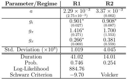
Table 1: US - GDP - QUARTERLY DATA - TWO REGIMES
In this section, I analyze the cases with 2 and 4 regimes, which give us the same general
conclusions had we used all models. In the appendix, the remaining models are detailed. I recall
that we have used the CBO proxy for calculating the output gap. The estimates with 2 regimes
are reported in table 1.
We observe first that both intercepts are statistically insignificant, and the coefficients of
the lagged interest rate are very similar. This shows no time-varying intercept, confirming what
Bueno (2005a) has encountered. Surprisingly, in the second regime, both the inflation and output
gap parameters are statistically insignificant, but in thefirst regime they have reasonable values.
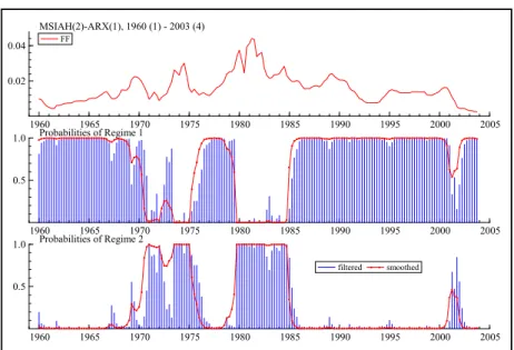
What is very interesting to observe is how these regimes are spread over time by looking at
figure 2.
We observe a very well characterized period after Greenspan, in which the inflation coefficient is superior to 1. However, this same behavior characterizes the 1960’s and the second half of the
1970’s, diverging from Clarida, Gal´ı and Gertler’s (2000) assumption. This clearly suggests that
the sample break proposed by the aforementioned is not that appropriate.
The other regime clearly characterizes the Vietnam War and the Volker-era, where the
coef-ficients are not significant. Thus, two things must be noticed from now on. The first is that the
last regime, which we are labelling Volcker-era, is always very well characterized,4 regardless the
number of regimes that we impose. Accordingly, when I increase the number of regimes, thefirst
4
Figure 2: TWO REGIMES PROBABILITIES - US
1960 1965 1970 1975 1980 1985 1990 1995 2000 2005 0.02
0.04
MSIAH(2)-ARX(1), 1960 (1) - 2003 (4) FF
1960 1965 1970 1975 1980 1985 1990 1995 2000 2005 0.5
1.0 Probabilities of Regime 1
1960 1965 1970 1975 1980 1985 1990 1995 2000 2005 0.5
1.0 Probabilities of Regime 2
filtered smoothed
regime is split into others. The second observation is that I always encounter non-significant
co-efficients for the Volcker-era, as the following table in this section and the tables in the appendix
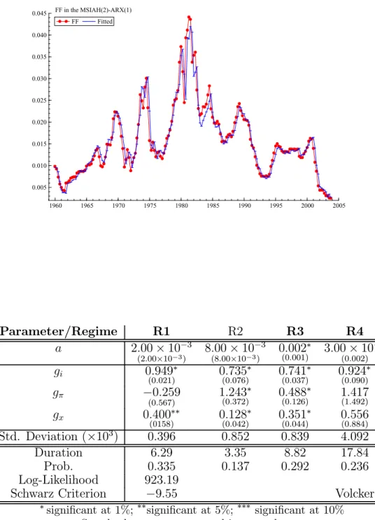
confirm. Looking at figure 3, we can observe how well the model fits the data.
If I increase the number of regimes to 4, I find weak evidence of time-varying intercept,
because, in general, they are very low and statistically insignificant. Although the inflation
parameter is significant in the intermediary regimes, it is greater than one only for the second
regime, which has the shortest duration and lowest probability.5 As a matter of fact, considering
what other empirical studies have reported, such as Orphanides (forthcoming), it is absolutely
unexpected to encounter many periods since the 1960’s in which the inflation coefficient is
non-significant or less than one.6 These results can be easily confirmed in table 2.
The output gap parameters have reasonable values and are significant in general. They reveal
different intensities, but always some effort to reduce output gap variability in compliance with the Kalman Filter estimates made by Bueno (2005a).
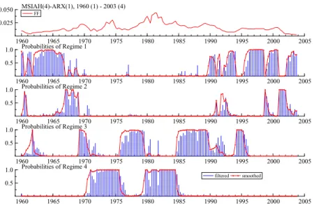
Figure 4 shows the temporal distribution of the regimes. Recall that in Regime 1, the inflation
parameter is non-significant and negative, and in regime 3 it is less than one; therefore, if one
5
This same pattern is found with 5 regimes.
6
Figure 3: MODEL FIT WITH 2 REGIMES - US
1960 1965 1970 1975 1980 1985 1990 1995 2000 2005 0.005
0.010 0.015 0.020 0.025 0.030 0.035 0.040
0.045 FF in the MSIAH(2)-ARX(1) FF Fitted
Parameter/Regime R1 R2 R3 R4
a 2.00×10⁻³
(2.00×10⁻³) 8.00×10
−3
(8.00×10⁻³) 0.002
∗
(0.001) 3.00×10
−3 (0.002)
gi 0.949∗
(0.021) 0.735
∗
(0.076) 0.741
∗
(0.037) 0.924
∗
(0.090)
gπ −0.259
(0.567) 1.243
∗
(0.372) 0.488
∗
(0.126) 1(1..417492)
gx 0.400∗∗
(0158) 0.128
∗
(0.042) 0.351
∗
(0.044) 0(0..556884)
Std. Deviation (×103) 0.396 0.852 0.839 4.092
Duration 6.29 3.35 8.82 17.84
Prob. 0.335 0.137 0.292 0.236
Log-Likelihood 923.19
Schwarz Criterion −9.55 Volcker
∗significant at 1%; ∗∗significant at 5%; ∗∗∗ significant at 10%
Standard errors are reported in parentheses.
takes into account that Greenspan has been leading the FED throughout most of these regimes,
one may be surprised. We also notice that it overlaps large portions of the findings of Sims and
Zha (2004, p. 22). In particular, my regimes 1, 3 and 4 correspond roughly to their regimes 1, 2
and 3, respectively .
Figure 4: FOUR REGIMES PROBABILITIES - US
1960 1965 1970 1975 1980 1985 1990 1995 2000 2005 0.025
0.050 MSIAH(4)-ARX(1), 1960 (1) - 2003 (4) FF
1960 1965 1970 1975 1980 1985 1990 1995 2000 2005 0.5
1.0 Probabilities of Regime 1
1960 1965 1970 1975 1980 1985 1990 1995 2000 2005 0.5
1.0 Probabilities of Regime 2
1960 1965 1970 1975 1980 1985 1990 1995 2000 2005 0.5
1.0 Probabilities of Regime 3
1960 1965 1970 1975 1980 1985 1990 1995 2000 2005 0.5
1.0 Probabilities of Regime 4
filtered smoothed
Generally speaking, the more regimes we allow for, then either the inflation coefficient greater than one is statistically non-significant, or less than one or, if significant and greater than one,
it demonstrates the shortest duration and lowest probability. Therefore, we argue that what
leads to a greater than one parameter are the few extreme observations that conceivably bias
the results toward a higher absolute value. This is a common problem discussed in the literature
and may be found, for instance, in the first chapter of Davidson and MacKinnon (1993). The
results also seem to be in disagreement with Orphanides (forthcoming), but clearly show that
there were regime switches in the US monetary policy, as documented by Sims and Zha (2004).
The findings here put under inquiry the results obtained by both Clarida, Gal´ı and Gertler
(2000) and Orphanides (forthcoming), because they diverge from them. In particular, I estimated
the Markov Switching Model with the same data set of Orphanides (forthcoming), assumingq = 0
and k= 1. Orphanides’ study is interesting because he has collected expected inflation reported
Hence, we can use directly observed expectations to estimate the model.
The tables are located in the appendix, but the analysis is discussed here. With two regimes,
the qualitative findings are identical to mine; with 3 regimes, the results start to deviate from
reasonable. For example, Ifindgπ <0 in the third regime, or very high, although non-significant
in the second regime. With 4 regimes, I find gi >1, and gπ either large, but non-significant, or
less than zero. In other words, with three and four regimes, Orphanides’ data demonstrates a
gπ >1 and significant in only one of the regimes. The shape of the pictures vary with respect to
mine, however they overall clearity of the last regime as representing the Volcker-era.
The general conclusion is that the theories supporting the Taylor Rule need to be further
developed to absorb the empirical results reported here. Anyone would disagree with the claim
that the US has indeterminate monetary dynamics. Thus, the puzzle is not in the data set, since
Bueno (2005a) has obtained similar results as Clarida, Gal´ı and Gertler (2000) using two other
estimation methods and the same sample break. Rather, this seeming incompatible finding,
that is the inflation coefficient less than one for most time of the sample, should refer to some
theoretical gap.
The results are even more striking if we observe that after the stabilization plan in Brazil,
the inflation parameter did not increase to one or above, as I will discuss in the next section.
4
EMPIRICAL RESULTS - BRAZIL
4.1
BRAZILIAN INTERVENTIONS
I suggest the expansion of the section 2 rule in order to take into account some important aspects
of Brazil. First, there were several stabilization plans during the period under analysis. They
should smooth price growth and, thus, the interest rates as I discuss in depth later on. There
were also two important structural changes in Brazil: first the Real Plan in 1994, which caused
the change from a high inflation level to one of low price growth; second, the exchange rate
modification from fixed to flexible rates in 1999. This envrionment is natural for experiments
to test theories assumed to work in distinct economic settings and with particular institutional
range:
Intervention Period Measure
Collor 1 Apr/90 to Aug/90 Abduction of financial assets
Collor 2 Mar/91 to Jun/91 Collor 1 + price control
Real Plan Jul/94 on New currency
Exchange Feb/99 on exchange fluctuation
Collor 1, Collor 2 and Real plans followed others aimed to stabilize the price level and failed.7
Policy makers dried the liquidity of the market freezing the amount of cash that people could
draw out of their own banking accounts in the first two plans. However, government started to
be sued and was forced by courts to release the money, making them to fail. Afiscal adjustment
preceded the third plan, which constituted a total indexation of the economy to the new unit
of value (URV). Once all contracts were indexed and the relative prices so adjusted, the old
currency was extinguished and Real replaced URV. Since then the inflation has been less than
1% a month on average. In February, 1999, exchange rate in Brazil became fullyflexible.
4.2
INTERNATIONAL RESERVES AND EXCHANGE RATE
Some, like Salgado, et alli (2001) among others, claim that the interest rate was also an
instru-ment to control changes over international reserves, such that interest rates responded to reserve
variations, which reflected the perception of the agents concerning which level the exchange rate
should be while it was fixed. Central Bank of Brazil reports appear to support this opinion.
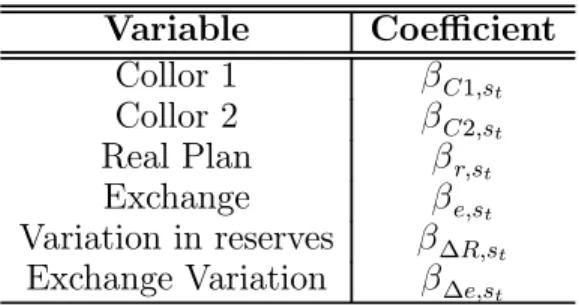
Therefore, I add variation of reserves and exchange rate and assume the following rule:
i∗t =i∗st+gπ,st[Et(πt,k)−π∗] +gx,stEt(xt,q) +X
0
tδst, (4)
where
Xt stands for a vector with the additional variables like dummies, reserves and exchange8;
7
The other plans were: Cruzado, from March/86 to Oct./86; Bresser, from July/87 to Sept./87; Summer, from Feb./89 to Apr./89. All those plans had a heterodox character of pegging prices someway. In general, they failed because there was nofiscal control and government always started to issue money again.
8
Variable Coefficient
Collor 1 βC1,st
Collor 2 βC2,st
Real Plan βr,st
Exchange βe,st
Variation in reserves β∆R,st
Exchange Variation β∆e,st
Table 3: CORRESPONDENCE BETWEEN COEFFICIENTS AND VARIABLES
δst is a vector of parameters corresponding to these variables.
Walsh (2003) or Taylor (1999) may provide a theoretical justification for the inclusion of such
variables.
Thus, combining the partial adjustment equation 2 with target model 4, I find the policy
reaction function:
it=ast+gi,stit−1 + (1−gi,st) (gπ,stEt(πt,k) +gx,stEt(xt,q)) +X
0
tβst+υt, (5)
where
ast = (1−gi,st)
¡
i∗st +gπ,stπ∗st
¢
;
βst = (1−gi,st)δst
9.
In order to collapse into the Taylor’s model, I assumek =q= 0. Table 3 maps each variable
that I add with its respective coefficient.10
4.3
DATA
For Brazil, I used the following quarterly data: SELIC Index for interest rates, Personal
Con-sumption Expenditure - IPCA for inflation and GDP. For monthly data, the same inflation and
interest rate measures are assumed, but I use the monthly GDP calculated by the Brazilian
Central Bank. As alternative proxies for this measure, I employ the consumption of Energy in
GWh and an Industrial production Index.
9
Since the focus of this paper is not on theδparameters, it is unnecessary to indentify them.
10
4.4
QUARTERLY DATA
I perform the same exercise with Markov-Switching for Brazil and report the results in this
section. The only model that I was able to estimate with quarterly data had 2 regimes. The
other models often did not converge, or presented overflow problems because of the restricted
number of observations available. Thus, later on I employ monthly data to check the robustness
of the results here. The output gap is obtained by quadratic detrending.
By looking at figure 5, one can perceive that the method effectively divides the periods
pre- and post-Real, which is highly expected from the method. The first regime represents the
post-Real Plan era, and the second, the pre-Real era. The transition between periods is nicely
depicted by the smoothed line. Moreover, from thefigure, one can conclude with the maintenance
of monetary policy over subsequent governments: from 1995 to 2002 with President Fernando
H. Cardoso, and from 2003 on, with President Lu´ıs I. Lula da Silva. This, of course, is in line
with the opinion of Brazilian people.
Figure 5: TWO REGIMES PROBABILITIES - QUARTERLY - GDP - BRAZIL
1995 2000 2005
0.5 1.0
MSIAH(2)-ARX(1), 1991 (2) - 2003 (4)
selic
1995 2000 2005
0.5
1.0 Probabilities of Regime 1
filtered smoothed
1995 2000 2005
0.5
1.0 Probabilities of Regime 2
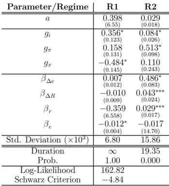
Table 4 shows the estimates.11 It is a surprise to observe the inflation parameter to be
non-11
Parameter/Regime R1 R2
a 0.398
(6.55) 0(0..029018)
gi 0.356∗
(0.123) 0.084
∗
(0.026)
gπ 0.158
(0.131) 0.513
∗
(0.098)
gx −0.484∗
(0.145) 0(0..110243)
β∆e 0.007
(0.012) 0.486
∗
(0.083)
β∆R −0.010
(0.009) 0.043
∗∗∗
(0.024)
βr −0.359
(6.558) 0.029
∗∗∗
(0.017)
βe −0.012∗
(0.004) −(140..01770)
Std. Deviation (×103) 6.80 15.86
Duration ∞ 19.35
Prob. 1.00 0.000
Log-Likelihood 162.82
Schwarz Criterion −4.84
∗significant at 1%; ∗∗significant at 5%; ∗∗∗ significant at 10%
Standard errors are reported in parentheses.
Table 4: BRAZIL - GDP - QUARTERLY DATA - TWO REGIMES
significant and less than one after the Real Plan, while before it was less than one (as theory
predicts), due to the presence of a sharp inflationary period.
Because of the small number of observations, I repeat the exercise with monthly data.
4.5
MONTHLY DATA
I estimate the Markov-Switching Regimes model for Brazil using 2, 3 and 4 regimes. I use three
proxies for output, but always quadratic detrending for obtaining the output gap: GDP, GWh
and an Industrial Production index. In this section, I report the results with GWh. Tables with
other proxies are shown in the appendix.
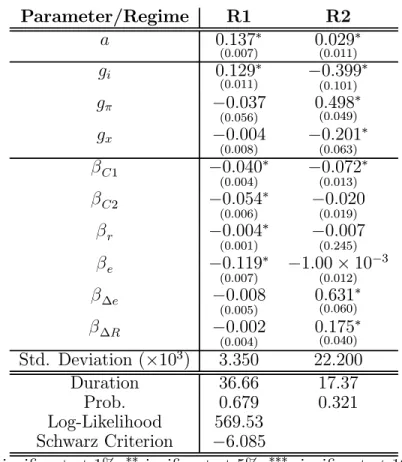
Table 5 shows some differences compared to the quarterly data; for instance, gi <0 and gx is
distinct between tables. However, the inflation parameter seems to be very close of each other.
From the table presented, we observe that the intercept is time-varying, and the reaction to
output gap is insignificant in the post-Real Plan period.
Figure 6 shows a very similar graph compared to quarterly data. In regime 1, the spikes
Parameter/Regime R1 R2
a 0.137∗
(0.007) 0.029
∗
(0.011)
gi 0.129∗
(0.011) −0.399
∗
(0.101)
gπ −0.037
(0.056) 0.498
∗
(0.049)
gx −0.004
(0.008) −0.201
∗
(0.063)
βC1 −0.040∗
(0.004) −0.072
∗
(0.013)
βC2 −0.054∗
(0.006) −(00..019)020
βr −0.004∗
(0.001) −(00..245)007
βe −0.119∗
(0.007) −1.00×10
−3 (0.012)
β∆e −0.008
(0.005) 0.631
∗
(0.060)
β∆R −0.002
(0.004) 0.175
∗
(0.040)
Std. Deviation (×103) 3.350 22.200
Duration 36.66 17.37
Prob. 0.679 0.321
Log-Likelihood 569.53
Schwarz Criterion −6.085
∗significant at 1%; ∗∗significant at 5%; ∗∗∗ significant at 10%
Standard errors are reported in parentheses.
results, based on the findings with quarterly data.
Figure 6: REGIME PROBABILITIES - MONTHLY DATA - GWh - BRAZIL
1990 1995 2000
0.25 0.50
MSIAH(2)-ARX(1), 1990 (2) - 2003 (12)
selic
1990 1995 2000
0.5
1.0 Probabilities of Regime 1
1990 1995 2000
0.5
1.0 Probabilities of Regime 2
filtered smoothed
Then I impose one more regime and estimate the parameters. Regime 2 comes out to represent
the spikes stressed infigure 6, the crises in the second half of the 90’s, and the transition between
regimes 1 and 3. (See figure 7.)
Exactly as in Bueno (2005a,b), which uses other estimation methods12, table 6 shows that
the lagged interest rate parameter becomes important after the Real Plan. At the same time,
the inflation parameter gradually loses importance. In addition, again a time-varying intercept
surfaces in thesefindings.
Imposing 4 regimes in the model, we perceive that regime 1 in previous models is once again
divided. A close look atfigure 8 reveals that its regimes 3 and 4 are similar to those found with
the model with 3 regimes. Regime 2 represents the transition period in 2003, when President
Lula took over the presidency, the transition from a fixed to flexible exchange rate regime in
1999, and other spikes not markedly characterized.
Table 7 provides no qualitative difference from previous analyses with 2 and 3 regimes. We do
not annoy the reader with more tedious words to stress the point that the results demonstrate the
12
Figure 7: THREE REGIMES PROBABILITIES - MONTHLY DATA - GWh - BRAZIL
1990 1995 2000
0.25 0.50
MSIAH(3)-ARX(1), 1990 (2) - 2003 (12)
selic
1990 1995 2000
0.5
1.0 Probabilities of Regime 1
1990 1995 2000
0.5
1.0 Probabilities of Regime 2
filtered smoothed
1990 1995 2000
0.5
1.0 Probabilities of Regime 3
Parameter/Regime R1 R2 R3
a 0.035∗∗
(0.014) 0.194
∗
(0.008) −0.017
∗∗∗
(0.009)
gi 0.811∗
(0.052) −0.011
∗
(0.023) 0.397
∗
(0.127)
gπ 0.127
(0.121) 0.277
∗
(0.018) 0.531
∗
(0.104)
gx −0.019
(0.014) −0.088
∗
(0.030) 0(0..098128)
βC1 −0.001
(0.125) −
0.161∗
(0.006)
0.012 (0.012)
βC2 −0.013
(0.068) −0.111
∗
(0.010) 0(0..015011)
βr −0.001
(4.00×10⁻³) −3.00×10
−3
(0.006) 0(7..107533)
βe −0.032∗
(0.013) −0.160
∗
(0.008) −0.082
∗∗∗
(0.044)
β∆e −0.001
(0.002) 0(0..013028) 0.399
∗
(0.051)
β∆R −0.003
(0.002) 0(0..004007) 0(0..052040)
Std. Deviation (×103) 1.306 2.674 15.334
Duration 21.07 2.93 16.54
Prob. 0.676 0.129 0.195
Log-Likelihood 698.56
Schwarz Criterion −7.17
∗significant at 1%; ∗∗significant at 5%; ∗∗∗ significant at 10%
Standard errors are reported in parentheses.
Figure 8: REGIME PROBABILITIES - MONTHLY DATA - GWh - BRAZIL
1990 1995 2000
0.25 0.50
MSIAH(4)-ARX(1), 1990 (2) - 2003 (12)
selic
1990 1995 2000
0.5
1.0 Probabilities of Regime 1
1990 1995 2000
0.5
1.0 Probabilities of Regime 2
1990 1995 2000
0.5
1.0 Probabilities of Regime 3
1990 1995 2000
0.5
1.0 Probabilities of Regime 4
filtered smoothed
ineffectiveness of the Taylor Rule in Brazil and that the results are not theoretically supported.
5
CONCLUSIONS
The results for the US turned out to be different during variations in the sample of the series. Any choice about where to start or to end a sample is arbitrary, and could distort the results that one
obtains. Therefore, I let the data itself choose different regimes and estimate the parameters of
the Taylor rule using Markov-Switching Regimes method, a completely new empirical approach,
which yields conclusions that contrast directly with those of Clarida, Gal´ıand Gertler (2000) and
with Orphanides (forthcoming). Again, I did not find any evidence of a time-varying intercept
for the US. The main (and surprising) finding is that the more regimes we allow for, then either
the inflation greater parameter than one is statistically non-significant, or less than one or, if
significant and greater than one, it has the shortest duration and the lowest probability. When
it is statistically significant and greater than one, this happens in unexpected periods like the
1960’s. These findings refute Clarida, Gal´ı and Gertler’s (2000) assumption about the break in
the series. As a consequence, the greater than one inflation parameter seems to be driven by the
Parameter/Regime R1 R2 R3 R4
a 0.065∗
(0.011) 0.100
∗
(0.014) 0.140
∗
(0.008) 0(0..008007)
gi 0.600∗
(0.054) 0.389
∗
(0.074) 0.137
∗
(0.023) 0.433
∗
(0.122)
gπ 0.050
(0.046) 0(0..011063) 0.370
∗
(0.014) 0(0..189160)
gx −0.010∗∗∗
(0.006) −(00.030).026 −0.052
∗∗
(0.025) 0(0..263160)
βC1 −0.036
(3.593) −0.041
∗
(0.002) −0.111
∗
(0.006) 0(0..006012)
βC2 −0.025
(0.015) −0.042
∗
(0.006) −0.074
∗
(0.007) 0(0..014113)
βr −0.001∗
(3.00×10−3) −0.005
∗
(0.001) −(00..006)001 0(0..104268)
βe −0.058∗
(0.011) −0.084
∗
(0.012) −0.107
∗
(0.008) −0.078
∗∗∗
(0.040)
β∆e 0.001
(0.003) −0.010
∗
(0.003) 0(0..007028) 0.562
∗
(0.050)
β∆R −0.003
(0.002) −0.010
∗∗
(0.004) −(00..008)006 0(0..016039)
Std. Deviation (×103) 1.010 1.252 2.268 11.675
Duration 23.27 4.11 3.05 8.58
Prob. 0.544 0.145 0.121 0.190
Log-Likelihood 711.12
Schwarz Criterion −6.80
∗significant at 1%; ∗∗significant at 5%; ∗∗∗ significant at 10%
Standard errors are reported in parentheses.
Then if we accept that most periods in the US economy existed an inflation parameter inferior
to one, this raises a theoretical question about the dynamic stability of the economy. On the
other hand, the reactions to output gap are almost always significant, revealing a permanent
concern of policy makers about reducing output gap variability, regardless of the econometric
model used, although with different intensities over time.
With quarterly data for Brazil, I estimated a Markov-Switching model with two regimes. I
confirmed all the results of Bueno (2005a, b) and observed a continuation of the monetary policy
after President Lula da Silva’s executive succession. With monthly data I was able to conclude the
existence of a time-varying intercept in Brazil (no matter the number of regimes that we impose),
and three very well pronounced regimes: high inflation regime (pre-Real Plan), transitory regime
during 1994/1995 when the Real Plan was implemented, and subsequent consistent monetary
policy just altered over a few months due to international crises or domestic exchange rate
surges13. We could also observe that the reaction to inflation is, in general, less than one or
insignificant, and it seems to approximate one in regimes where high inflation was predominant.
By contrast, the coefficient for the lagged interest rate becomes high and significant in the post-Real plan regimes, in compliance with the results using the Kalman Filter and nonlinear least
squares (see Bueno, 2005a, b).
Overall, two conclusions emerge. Theoretically, there is space for further research into
co-herent explanations regarding the results obtained here. Practically, one can conclude that the
Taylor Rule may be ineffective to conduct monetary policy. This is particularly important in
Brazil, because there there is a widespread feeling among people that the conduction of monetary
policy does not work at all. The Central Bank has increased the interest rate for several months
between September/2004 and May/2005 without success in terms of reducing the inflation.
We point out that our results are in line with Sims and Zha (2004) who find different regimes
for US monetary policy, and hence different coefficients. Thus other studies on monetary rules
must take into account this data particularity.
13
References
[1] ARNOLD, Dennis. A Summary of Alternative Methods for Estimating Potential GDP.
Washington, DC: Congressional Budget Office, 2004.
[2] BUENO, Rodrigo D. L. S. Questioning the Taylor Rule: Hidden variables. Working Paper:
University of Chicago, 2005.
[3] BUENO, Rodrigo D. L. S. The Ineffectiveness of the Taylor Rule. Working Paper: University
of Chicago, 2005.
[4] CATI, Regina C., GARCIA, Marcio G. P. & PERRON, Pierre. Unit Roots in the
Pres-ence of Abrupt Interventions with an Application to Brazilian Data. Journal of Applied
Econometrics, vol. 14, n.o 1; pp. 27-56, 1999.
[5] CLARIDA, Richard, GAL´ı, Jordi & GERTLER, Mark. Monetary Policy Rules and
Macroe-conomic Stability: Evidence and some theory.Quarterly Journal of Economics, vol. 115, n.o
1, pp. 147-80, 2000.
[6] DAVIDSON, Russel & MACKINNON, James G.Estimation and Inference in Econometrics.
New York: Oxford, 1993.
[7] DICKEY, David A. & PANTULA, Sastry G. Determining the Order of Differencing in
Autoregressive Processes. Journal of Business & Economic Statistics, vol. 5, n.o 4, 455-61,
1987.
[8] HAMILTON, James D. Time Series Analysis. Princeton: Princeton, 1994.
[9] HARRIS, Richard I. D.Cointegration Analysis in Econometric Modelling. Englewood Cliffs:
Prentice Hall, 1995.
[10] KROLZIG, Hans-Martin. Markov-Switching Vector Autoregressions. Berlin:
Springer-Verlag, 1997.
[11] ORPHANIDES, Athanasios. Monetary Policy Rules, Macroeconomic Stability and Inflation:
[12] PHILLIPS, Peter & PERRON, Pierre. Testing for a Unit Root in Time Series Regression.
Biometrika, vol. 75, n.o 2, p.p. 335-346, 1988.
[13] SIMS, Christopher A. & ZHA, Tao. Were There Regime Switches in US Monetary Policy?
Princeton University: Working paper, 2004.
[14] TAYLOR, John. B. Discretion versus Policy Rules in Practice. Carnergie-Rochester
Con-ference Series on Public Policy, vol. 39, p.p. 195-214, 1993.
[15] TAYLOR, John B. Monetary Policy Rules. Chicago: The University of Chicago Press and
NBER, 1999.
[16] WALSH, Carl E. Monetary Theory and Policy, 2nd. ed. Cambridge, MA: MIT Press, 2003.
[17] WOODFORD, Michael. Optimal Monetary Policy Inertia. Unpublished, Princeton
Univer-sity, 1999.
Series Pot. GDP GDP PCE EFFR
qn q P
t i
Source CBO BEA BEA BG
Seas. Adj. NA YES YES NA
Freq. Q Q Q M
Units B 2000 US B 2000 US 2000 = 100 %
Range 1949-2014 1947-2003 1947-2003 1954-2004
BEA U.S. Department of Commerce: Bureau of Economic Analysis
BG Board of Governors of the Federal Reserve System
CBO U.S. Congress: Congressional Budget Office
PCE Personal Consumption Expenditures: Chain-type Price Index
EFFR Effective Federal Funds Rate
NA Not applicable
Table 8: DATA DESCRIPTION - USA
qn q i π
Mean 6.99 6.97 0.015 0.009
Std. Dev. 0.53 0.55 0.008 0.007
Skewness −0.16 −0.14 1.105 0.974
Kurtosis 1.82 1.85 4.414 4.094
#Obs. 220 228 198 227
Table 9: BASIC STATISTICS - US
APPENDIX A: DATA DESCRIPTION
UNITED STATES
This section is designed to define the data source and to give the basic statistics of the data I
am using. Income and output are always in constant prices. The data-source that we use for the US is summarized in table 8.
Some basic statistics about these variables are presented in table 9. All variables are in log terms.
I proceed the Phillips-Perron unit root test (see Phillips and Perron, 1988) with trend and intercept, unless otherwise noticed.14 See table 10.
14
For simplicity, I do not follow Dickey and Pantula’s (1987) procedure here.
Variable Levels 1.st
Differences
q −2.49 −10.65∗,b
i −2.34b −10.91∗,c
π −4.80∗,b
∗- Significant at 1% level
b - Without trend; c - Without trend and intercept
Series GDP IPCA SELIC Cons. Energy PINDEX Reserves Exchange
q π i GW h IND Res d
Source BCB IPEA IPEA Eletrobr´as IBGE BCB BCB
Seas. Adj. YES YES NA YES YES NA NA
Freq. Q/M M M M M M M
Units B 2003 Real 1990 = 100 % GWh 2002 = 100 US$ B R$/US$
Range 1991-2003 1947-2003 1974-2004 1979-2004 1991-2004 1970-2005 1990-2004
BCB Central Bank of Brazil NA Not applicable
IPCA Consumer Price Index PINDEX Production Index
IPEA Applied Research Economics Institute IBGE Brazilian Institute of Statistics SELIC Effective Federal Funds Rate
Table 11: Data Description
Quarterly π q i
Mean 0.20 26.53 0.24
Std. Dev. 0.31 0.10 0.33
Skewness 1.39 −0.54 1.48
Kurtosis 3.36 2.03 3.70
# Obs. 52 52 52
Table 12: BASIC STATISTICS - BRAZIL
I also ran the Johansen’s cointegrating test among q, π, and i (see Harris, 1995.) I rejected the hypothesis of no cointegration using both trace and max-eigenvalues statistics, with intercept and no trend, but I do not report the results.
The Johansen’s test allows me to use the variables at their individual levels. But I could
simply assume that interest rate is stationary as in Clarida, Gal´ı e Gertler (2000), because of
the empirical plausibility of this assumption, as well as the low power of the unit root tests. Moreover, stationarity is also a property found in many theoretical models.
APPENDIX B: BRAZILIAN DATA DESCRIPTION
BRAZIL
The data used in this work is described in table 11.
Some basic statistics about these variables are presented in table 12.
I proceed the Phillips-Perron unit root test in table 13 with trend and intercept, unless otherwise noticed.
Although I do not report results, we carried out Johansen’s cointegration test and whatever the hypothesis regarding trend and intercept, linear or quadratic, there is always at least one cointegrating vector.15
15
Variable Levels First Differences
q −2.70 −6.16∗,b
π −2.25 −5.21∗,b
i −2.61 −6.96∗,b
∗- Significant at 1% level; b - Without trend
Table 13: UNIT ROOT TESTS - Quarterly - BRAZIL
Monthly π i q GW h IND
Mean 0.08 0.09 10.73 9.96 4.49
Std. Dev. 0.12 0.12 0.24 0.15 0.10
Skewness 1.81 1.66 0.31 −0.23 −0.53
Kurtosis 6.15 5.12 1.85 1.67 2.74
#Obs. 171 171 171 171 158
Table 14: BASIC STATISTICS - BRAZIL
Basic statistics for monthly data are in table 14.
I proceed the Phillips-Perron unit root test with trend and intercept, unless otherwise noted in table 15
APPENDIX C: MARKOV-SWITCHING - US
3 REGIMES - US
5 REGIMES - US
APPENDIX D: ORPHANIDES DATA
Orphanides data is annualized. That’s why the standard deviation seems higher.
Variable Levels First Differences
q -1.36 -12.59b,∗
π -4.30∗ −
i -4.36∗ −
GW h -2.79 -14.28b,∗
IND -5.69∗
-∗- Significant at 1% level; b - Without trend
Parameter/Regime R1 R2 R3
a 1.00×10⁻³
(2.00×10⁻³) −4.00×10
−3
(5.00×10⁻³) 0(0..005005)
gi 0.959∗
(0.022) 0.849
∗
(0.038) 0.839
∗
(0.131)
gπ −0.364
(0.649) 1.350
∗
(0.308) 0(1..081001)
gx 0.436∗∗
(0.212) 0.259
∗
(0.076) 0(0..369419)
Std. Deviation (×103) 0.384 1.399 4.546
Duration 5.68 7.53 13.42
Prob. 0.319 0.515 0.166
Log-Likelihood 903.58
Schwarz Criterion −9.65 Volcker
∗significant at 1%; ∗∗significant at 5%; ∗∗∗ significant at 10%
Standard errors are reported in parentheses.
Table 16: US - GDP - QUARTERLY DATA - THREE REGIMES
Figure 9: THREE REGIME PROBABILITIES - US
1960 1965 1970 1975 1980 1985 1990 1995 2000 2005 0.02
0.04
MSIAH(3)-ARX(1), 1960 (1) - 2003 (4) FF
1960 1965 1970 1975 1980 1985 1990 1995 2000 2005 0.5
1.0 Probabilities of Regime 1
1960 1965 1970 1975 1980 1985 1990 1995 2000 2005 0.5
1.0 Probabilities of Regime 2
1960 1965 1970 1975 1980 1985 1990 1995 2000 2005 0.5
1.0 Probabilities of Regime 3
Parameter/Regime R1 R2 R3 R4 R5
a 0.00×10⁻³
(2.00×10⁻³) −7.00×10
−3
(5.00×10⁻³) 9.00×10
−3∗∗
(3.00×10⁻³) −(00.003).003 0(0..007004)
gi 0.954∗
(0.019) 0.768
∗
(0.053) 0.846
∗
(0.029) 0.819
∗
(0.080) 0.825
∗
(0.128)
gπ
1−gi −(00.503).050 1.003 ∗
(0.362) 0.735
∗
(0.151) 2(1..124572) −(00..925)183
gx
1−gi 0.470
∗∗
(0196) 0.076
∗∗
(0.038) 0.397
∗
(0.008) 0.313
∗∗∗
(0.172) 0(0..395405)
Std. Deviation (×103) 0.383 0.583 0.804 1.569 4.553
Duration 6.20 2.45 9.88 7.49 14.00
Prob. 0.318 0.094 0.301 0.130 0.158
Log-Likelihood 928.97
Schwarz Criterion −9.24 Volcker
∗significant at 1%; ∗∗significant at 5%; ∗∗∗ significant at 10%
Standard errors are reported in parentheses.
Table 17: US - GDP - QUARTERLY DATA - FIVE REGIMES
Figure 10: FIVE REGIMES PROBABILITIES - US
1960 1965 1970 1975 1980 1985 1990 1995 2000 2005 0.025
0.050 MSIAH(5)-ARX(1), 1960 (1) - 2003 (4)
FF
1960 1965 1970 1975 1980 1985 1990 1995 2000 2005 0.5
1.0 Probabilities of Regime 1
1960 1965 1970 1975 1980 1985 1990 1995 2000 2005 0.5
1.0 Probabilities of Regime 2
1960 1965 1970 1975 1980 1985 1990 1995 2000 2005 0.5
1.0 Probabilities of Regime 3
1960 1965 1970 1975 1980 1985 1990 1995 2000 2005 0.5
1.0 Probabilities of Regime 4
1960 1965 1970 1975 1980 1985 1990 1995 2000 2005 0.5
Parameter/Regime R1 R2
a −0.194
(0.213) 0(0..244860)
gi 0.930∗
(0.032) 0.860
∗
(0.081)
gπ
1−gi 3.214
∗∗
(1.393) 2(1..050519)
gx
1−gi 1.785
∗∗∗
(0.939) 0(0..251701)
Std. Deviation 0.480 1.933
Duration 17.24 10.07
Prob. 0.631 0.369
Log-Likelihood −156.32
Schwarz Criterion 3.19
∗significant at 1%; ∗∗significant at 5%; ∗∗∗ significant at 10%
Standard errors are reported in parentheses.
Table 18: US - ORPHANIDES GDP - QUARTERLY DATA - TWO REGIMES - EXPECTED INFLATION (k = 1, q = 0)
Figure 11: TWO REGIMES PROBABILITIES - ORPHANIDES DATA SET - (k = 1, q = 0)
1970 1975 1980 1985 1990 1995
5 10 15
20 MSIAH(2)-ARX(1), 1967 (1) - 1995 (4) FF
1970 1975 1980 1985 1990 1995
0.5
1.0 Probabilities of Regime 1
1970 1975 1980 1985 1990 1995
0.5
1.0 Probabilities of Regime 2
Parameter/Regime R1 R2 R3
a 0.317
(0.283) −(00.370).249 37.750
∗
(0.624)
gi 0.792∗
(0.027) 0.993
∗
(0.039) −(00..302)321
gπ 1.581∗
(0.368) (8415..172)53 −1.384
∗∗
(0.619)
gx 0.958∗
(0.220) −(224..522)972 0.608
∗
(0.153)
Std. Deviation 0.409 0.624 1.644
Duration 2.72 3.10 4.070
Prob. 0.367 0.678 0.239
Log-Likelihood −138.49
Schwarz Criterion 3.25
∗significant at 1%; ∗∗significant at 5%; ∗∗∗ significant at 10%
Standard errors are reported in parentheses.
Table 19: US - ORPHANIDES GDP - QUARTERLY DATA - THREE REGIMES - EXPECTED INFLATION (k = 1, q = 0)
Figure 12: THREE REGIMES PROBABILITIES - ORPHANIDES DATA SET - EXPECTED INFLATION (k = 1, q = 0)
1970 1975 1980 1985 1990 1995 5
10 15
20 MSIAH(3)-ARX(1), 1967 (1) - 1995 (4) FF
1970 1975 1980 1985 1990 1995 0.5
1.0 Probabilities of Regime 1
1970 1975 1980 1985 1990 1995 0.5
1.0 Probabilities of Regime 2
1970 1975 1980 1985 1990 1995 0.5
1.0 Probabilities of Regime 3
Parameter/Regime R1 R2 R3 R4
a −0.447∗∗
(0.211) 0(0..426305) −(00..624)378 38.241
∗
(11.222)
gi 1.053∗
(0.023) 0.777
∗
(0.032) 0.999
∗
(0.052) −0.342
∗
(0.326)
gπ −2.218
(1.763) 1.571
∗
(0.380) (385,694.083.004) −1.373
∗∗∗
(0.744)
gx −2.659∗
(0.979) 0.926
∗
(0.234) −(2,56404..667580) 0.613
∗
(0.163)
Std. Deviation 0.228 0.390 0.655 1.648
Duration 2.03 2.32 2.45 4.04
Prob. 0.199 0.347 0.385 0.070
Log-Likelihood -131.98
Schwarz Criterion 3.59
∗significant at 1%; ∗∗significant at 5%; ∗∗∗ significant at 10%
Standard errors are reported in parentheses.
Table 20: US - ORPHANIDES GDP - QUARTERLY DATA - FOUR REGIMES - EXPECTED INFLATION (k = 1, q = 0)
Figure 13: FOUR REGIME PROBABILITIES - ORPHANIDES DATA SET - EXPECTED INFLATION (k = 1, q = 0)
1970 1975 1980 1985 1990 1995
10
20 MSIAH(4)-ARX(1), 1967 (1) - 1995 (4)FF
1970 1975 1980 1985 1990 1995
0.5
1.0 Probabilities of Regime 1
1970 1975 1980 1985 1990 1995
0.5
1.0 Probabilities of Regime 2
1970 1975 1980 1985 1990 1995
0.5
1.0 Probabilities of Regime 3
1970 1975 1980 1985 1990 1995
0.5
1.0 Probabilities of Regime 4
Parameter/Regime R1 R2
a 0.140∗
(0.007) 0(0..005013)
gi 0.125∗
(0.011) −0.455
∗
(0.104)
gπ −0.040
(0.054) 0.542
∗
(0.047)
gx −0.008∗∗∗
(0.005) −0.061
∗
(0.017)
βC1 −0.040∗
(0.040) −0.036
∗∗
(0.017)
βC2 −0.057∗
(0.006) −(00..033)022
βr −0.006∗
(0.001) −(00..216)035
βe −0.121∗
(0.007) 0.038
∗∗
(0.015)
β∆e −0.011∗∗
(0.005) 0.659
∗
(0.060)
β∆R −0.001
(0.004) 0.172
∗
(0.040)
Std. Deviation (×103) 3.284 21.969
Duration 31.12 15.49
Prob. 0.675 0.325
Log-Likelihood 571.59
Schwarz Criterion −6.11
∗significant at 1%; ∗∗significant at 5%; ∗∗∗ significant at 10%
Standard errors are reported in parentheses.
Table 21: BRAZIL - Gdp - MONTHLY DATA - TWO REGIMES
APPENDIX E: MARKOV-SWITCHING - BRAZIL
I present only the results with GDP because they are identical to using the Indutrial Production Index - IND.
Figure 14: TWO REGIME PROBABILITIES - MONTHLY DATA - GDP - BRAZIL
1990 1995 2000
0.25 0.50
MSIAH(2)-ARX(1), 1990 (2) - 2003 (12)
selic
1990 1995 2000
0.5
1.0 Probabilities of Regime 1
1990 1995 2000
0.5
1.0 Probabilities of Regime 2
filtered smoothed
Parameter/Regime R1 R2 R3 R4
a 0.141∗
(0.000) 0.090
∗
(0.007) 0.175
∗
(0.008) −4.00×10
−3 (0.007)
gi −0.020∗
(1.00×10−3) 0.799
∗
(0.035) −(00..092)104 0.397
∗
(0.090)
gπ −0.086∗
(0.69×10−3) 0(0..093091) 0.333
∗
(0.051) 0.746
∗
(0.072)
gx 0.005∗
(0.16×10−3
) 0(0..006010) 0.028
∗
(0.008) 0(0..014024)
βC1 −0.037∗
(0.000) 0.111
∗
(0.006) −0.136
∗
(0.014) −2.00×10
−3 (0.011)
βC2 −0.034∗
(0.000) 0.113
∗
(0.004) −0.087
∗
(0.000) −(00.176).010
βr −0.013∗
(0.000) −1.00×10
−3
(0.001) −(00..033)011 0(0..124132)
βe −0.110∗
(0.000) 0.093
∗
(0.007) −0.141
∗
(0.007) −0.117
∗
(0.033)
β∆e 0.104∗
(0.000) −(00..002)001 −0.095
∗
(0.028) 0.222
∗
(0.050)
β∆R 0.014∗
(0.000) −(00..002)002 −(00..010)010 0(0..019028)
Std. Deviation (×103) 0.006 1.267 2.751 9.691
Duration 1.81 16.02 5.62 14.30
Prob. 0.073 0.643 0.080 0.204
Log-Likelihood 784.36
Schwarz Criterion −7.68
∗significant at 1%; ∗∗significant at 5%; ∗∗∗ significant at 10%
Standard errors are reported in parentheses.
Figure 15: FOUR REGIMES PROBABILITIES - MONTHLY DATA GDP - BRAZIL
1990 1995 2000
0.25 0.50
MSIAH(4)-ARX(1), 1990 (2) - 2003 (12)
selic
1990 1995 2000
0.5
1.0 Probabilities of Regime 1
1990 1995 2000
0.5
1.0 Probabilities of Regime 2
1990 1995 2000
0.5
1.0 Probabilities of Regime 3
1990 1995 2000
0.5
1.0 Probabilities of Regime 4