Hierarchical Compressed Sensing for Cluster Based Wireless Sensor Networks

Hierarchical Compressed Sensing for Cluster Based

Wireless Sensor Networks

Vishal Krishna Singh

Dept. of Information Technology Indian Institute of Information Technology

Allahabad, India

Manish Kumar

Dept. of Information Technology Indian Institute of Information Technology

Allahabad, India

Abstract—Data transmission consumes significant amount of energy in large scale wireless sensor networks (WSNs). In such an environment, reducing the in-network communication and distributing the load evenly over the network can reduce the overall energy consumption and maximize the network lifetime significantly. In this work, the aforementioned problem of network lifetime and uneven energy consumption in large scale wireless sensor networks is addressed. This work proposes a hierarchical compressed sensing (HCS) scheme to reduce the in-network communication during the data gathering process. Co-related sensor readings are collected via a hierarchical clustering scheme. A compressed sensing (CS) based data processing scheme is devised to transmit the data from the source to the sink. The proposed HCS is able to identify the optimal position for the application of CS to achieve reduced and similar number of transmissions on all the nodes in the network. An activity map is generated to validate the reduced and uniformly distributed communication load of the WSN. Based on the number of transmissions per data gathering round, the bit-hop metric model is used to analyse the overall energy consumption. Simulation results validate the efficiency of the proposed method over the existing CS based approaches.

Keywords—Compressed sensing; in-network communication; network lifetime; traffic load balancing; wireless sensor network

I. INTRODUCTION

Wireless sensor networks (WSNs) have revolutionised today's practice of numerous scientific and engineering endeavours, including ecosystems, environmental sciences, military applications, scientific research etc. WSNs are used for sensing physical variables of interest at unprecedented high spatial densities and long-time durations [1]. Applications like environmental monitoring, scientific research etc., explore the benefits of WSNs. Such applications require transferring a huge amount of sensed data from one point of the network to another. Considering the fact, that the energy consumed in transmission of 1 Kb of data over a distance of 100 meters is equal to the energy consumed in executing 300 million instructions with the rate of computation being 100 million instructions per second on a processor with general configurations [3], [4]. Almost 70% of the total energy is consumed in communication within the network [2]. Hence, the inherent constraints of WSNs such as limited bandwidth and limited battery life makes them prone to failure and compromise the network lifetime. Significant energy conservation in such networks can be achieved by: a) minimizing the cost of interaction between the nodes and b)

achieving traffic load balancing during in-network communications [3]. Techniques such as data aggregation have been used to efficiently reduce the communication load of the network, however the issue of asymmetric load distribution in the network remain an important concern till date. Load balancing and optimized energy consumption are thus, much sought after parameters for multi hop data transmission in WSNs.

This work addresses the problem of uneven energy consumption and network lifetime maximization through a novel in-network data processing scheme which incorporates CS in a novel way over a clustered routing structure. The nodes are randomly deployed in a sensing area which is divided into homogenous sub-regions. Such a division is done to model the real world scenario of an area such as a thermal power plant. In such a deployment, the area can be divided into homogeneous regions in such a way that one homogeneous region is different from the other.

For example, the area with the thermal station (one homogeneous region) will exhibit high temperature readings as compared to the residential areas of the plant (another homogeneous region) and are known as a priori. The proposed HCS is divided into two phases, a) Clustering and communication phase b) CS and data processing phase. The proposed scheme incorporates CS in a way to efficiently distribute the communication load evenly over the network. To the best of our knowledge, the advantages of using CS and hybrid CS on tree based routing structure are many but its advantages over a clustered routing structure have not been explored yet. The contributions of this work can be summarised as:

 A CS based data processing scheme with minimum in-network transmissions.

 A scheme for enhancing the network lifetime by balanced network traffic load distribution

II. RELATED WORK

Data aggregation in WSNs is considered to be the most easily deployable data reduction technique [2]. With varying network topology, such as cluster based [2], tree based [3], chain based [4], various data aggregation schemes have been proposed [4], [5], [6], [7], [8], [9]. Data aggregation mainly exploits the redundancy in the spatially and temporally co-related data sensed by the nodes [10]. Hence, significant energy conservation is achieved by reducing the amount of data being forwarded by any node. However, data aggregation approaches suffer from certain disadvantages. The most important concern with most of the data aggregation approaches, is the loss of information. Data aggregation approaches mainly focus on transferring only a summary of the sensed value to the sink. Hence, a lot of information about the measured value is sacrificed by the aggregation techniques [11]. Another drawback of data aggregation schemes is the asymmetric load distribution within the network. This results in parts of the network having relatively higher activity and thus becoming non-operational because of dead nodes, leaving the sink isolated. For example, in case of an event, WSNs have large amount of data flowing in the network. In such an environment, activity in the deployment area depends upon the occurrence of an event and position of the nodes [12]. The nodes near the sink have high energy consumption as compared to the nodes in other region because of heavy load of data transmission to the sink. Asymmetric distribution of the load results in high activity in parts of the network causing nodes with heavy communication load to die quickly.

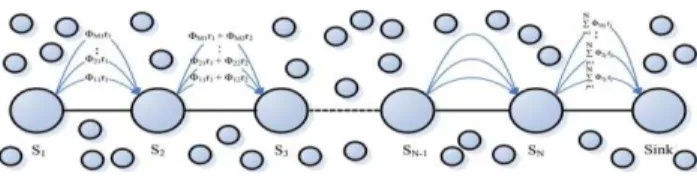
Fig. 1. Traditional data gathering in multi-hop environment

CS has evolved as a promising technique, which can efficiently overcome the drawbacks of the existing aggregation approaches. Data gathering in traditional multi hop environment can be understood from the Fig 1. which shows the highlighted path in a WSN where, „N‟ sensor nodes form a multi-hop path for data collection. Let the reading generated by the node S1 is r1. Similarly, reading generated by the node S2 is r2 and so on. In a normal data acquisition process, the node S1 sends its reading to node S2. S2 in turn transmits both its data r2 and the data obtained from S1 to S3 .Finally in the end, the last node of the route, sends all the data received from previous nodes along with its own data to the sink. As seen in the Fig.1, the nodes closer to the sink consume more energy as compared to the nodes away from the sink. Due to this, the nodes closer to sink will be drained quickly compromising the lifetime of the network.

Fig. 2. Data gathering with Compressed Sensing

The Fig. 2 shows the compressed data gathering method in

the highlighted path of a WSN where, „N‟ sensor nodes form a

multi-hop path for data collection. The sink upon receiving all

the M samples from „N‟ nodes, reconstructs the original data.

In order to send the ith sample to the sink, S1 generates a random coefficient



_i1 and multiplies it‟s reading i.e. r1 with it. The product is then sent to the node S2. Similar multiplication is performed at the node S2 with the random coefficient Φ_i2and the sumΦ_{i1 1}r  Φ_{i2 2}r is sent to the node S3. This process is followed by every node in the route to send M samples of their data. Such a transmission results in the sink receiving Φ

1

n r ij j j



 . The number of samples sent by each node is

scheme. The authors divide the nodes in a clustered fashion to transmit the compressed data through various levels.

Thus, variations of CS have proved to be advantageous in such an environment as WSN, but the existing approaches have certain disadvantages. An important concern is that most of the existing work on CS view compression from the signal processing perspective only [21], [22]. Applications on data compression, from the networking protocol perspective in WSNs are limited [23]. CS, if and when applied naively to a sensor network, imposes extra burden over the network. As shown in Fig. 2, suppose

N



1

nodes are each sending one sample to the Nth node, the outgoing link of that node will

carry „N‟ samples if no aggregation is performed; or will carry

1 sample if lossy aggregation is performed. If we apply the CS principle directly, the CS aggregation will force every link to

carry „M‟ samples, leading to unnecessary higher traffic at the

early stage transmissions [13]. To overcome these drawbacks, the idea of hybrid CS was proposed but hybrid CS has its own disadvantages. The selection of non-CS and CS points within the hybrid-CS scheme is critical in getting the benefit of CS [13], [14], [15]. Distributed CS [23] suffers as compared to a mixed protocol in large-scale WSNs, under real technological constrains. Unless the network size and compression are both taken into consideration in network design, distributed CS approaches tend to have average performance in terms of lifetime and energy conservation. Interestingly, existing works on compressed data gathering in WSNs, mainly exploit the tree based routing structure. Because of the drawbacks of the tree based routing structure, such as unstable network topology, most of the existing works face the problem of unreliability and poor quality of service [26].

Thus, the proposed HCS is developed on the principle of hybrid CS over clustered routing structure, with the aim of achieving reliable data transmission with minimum energy consumption (achieved by minimizing and balancing the network traffic evenly over the network).

III. PROBLEM DEFINITION

The main objective in WSNs is to reduce the in-network communication and improve the throughput of the network by increasing the network lifetime. However, network lifetime in large scale wireless sensor networks is also significantly affected by uneven energy expenditure by sensor nodes. Nodes with heavy communication load consume more energy and die quickly causing holes and isolation of some regions of the network. It is therefore desirable to process as much data locally as possible so as to reduce the number of bits transmitted. Techniques such as data aggregation are used to reduce the amount of data being forwarded by the nodes. However, data aggregation schemes have certain drawbacks such as, asymmetric load distribution and information loss. In case of an event, WSNs have large number of message transmissions in the network. In such an environment, activity in the deployment area depends upon the occurrence of an event and position of the nodes. The nodes near the sink have high energy consumption as compared to the nodes in other regions because of heavy load of data transmission to the sink. An asymmetric distribution of the load results in parts of the network having relatively higher activity and thus becoming

non-operational because of dead nodes, leaving the sink isolated. Energy conservation may be achieved by transmitting only the summary of the sensed data that may result loss of information. Recent reported work state that, the idea of using CS for data transmission can be advantageous in the above scenario. Naïve application of CS to a sensor network imposes extra burden over the network, hence Hybrid CS would be the most suited solution. However, determining the CS and non-CS points is crucial in such approaches to explore the true potential of the scheme. Hence a CS scheme with the ability of uniform load distribution and efficient data transmission is desired. Reduced in-network communication and optimized energy usage in such a scheme will significantly improve stability period and reduced instable region. Hence, a scheme based on compressed sensing over clustered routing structure is proposed.

IV. PROPOSED APPROACH A. Compressed sensing

The idea of compressive data gathering is relatively new in the field of wireless sensor networks. Some of the basic yet essential properties of the framework asserts that, a relatively small number of samples of a sparse data contains enough information to successfully recover the original data with almost no data loss [27]. Mathematically, If a sparse data „

x

‟

can be denoted as



1, 2 3



T

,

..

N

x



x x x



x

such that

N

x



R

and the orthogonal sparse basis or projection ofxis given by

      



₁

,

₂

,

₃

..

_N



where



_iis the ith

column of



, then x can be given by the following equation:

1

.

N

i i

i

x

S

S



  





(1)

Such that, S is a vector of the coefficient matrix



and “.” represents the inner product. According to the theory of the CS, provided the target dataxis K-sparse in the basis



, then under specific conditions, M adaptive measurements ofx are sufficient to fully recover the original data such that

M



. Where each weighted measurement, y, can be written as:

Φ

y



x

(2)

The recovery of the target data by M measurements is dependent on the following condition:





2

.

Φ . .

M



c





K logN

(3)

Where

Φ

is a

M



N

sensing matrix, „c‟ is a positive

constant and



(

Φ )



is the coherence between the sensing matrix

Φ

and the representation basis



. The original data is recovered by solving a convex optimization problem, given by:

(

1

_i

)

i

l

s





s

1

n

min

s

ò

R

s l

And considering,

^

Ψ

x



s

_{, with}

s

^ _{being the optimal}

solution.

Thus, an important conclusion can be drawn from the assertion is that the basic foundation of CS relies on sensing matrices. For reliable and efficient compression, the data must be sparse in some intitutively known domain and the sensing matrix,

Φ

, must meet the restricted isometric property (RIP).

An essential property of the sensing matrix,

Φ

, is the Null space property (NSP) and is denoted by:

  

Φ : 0 . NSP



N  z Az 

To explain, a sparse data x, can be completely recovered by

Φx

, if for every pair of distinct vectors such as ,x x' , k





'

Φx = Φx

. Considering the mentioned condition is not true i.e. if Φx = Φx' , results

Φ



x



x

'





0

such that

'

2k

.

x

 

x



Therefore, it can be said that for „A‟ to

uniquely represent every k

x





,

N

(

Φ)

should not contain

a vector that belongs to 2k



. This feature of the sensing matrix is known as spark of the matrix and is defined as:

Definition 1. The spark of a sensing matrix given by

Φ

, is the smallest number of linearly dependent columns of

Φ

.

Theorem 1. If the spark of a sensing matrix

Φ

, is greater than

2

k

then, for a given vector, y, where

y



R

m, there exists a unique data

x





_k

,

such that

y



Φ

x

.

Proof: To prove the theorem 1 by contradiction, let there

be a vector „y‟ such that

y



R

mand there exists a unique

data

,

k

x





such that

y



Φ

x

. It is assumed that, spark

( )

 

2

k

. Or it can be said that there are at most

2

k

linearly independent columns which implies that there is an

(

Φ)

h N



such that

2

.

k

h





Now, since ₂ ,

k

h



therefore

h

 

x x

'

, where

x x

, '





_k

.

As we know that

(

Φ)

h N



, therefore

Φ

 

x x



'



0

and

Φ

x



Φ

x

'. But this is a contradiction of the above assumption that there exists a unique data

x





_k

,

such that

y



Φ

x

. Hence, spark

( )

 

2

k

. Now, considering spark

( )

 

2

k

, and for a

given „y‟ there exist

x x

, '





_k

,

such that:

Φ Φ



x



Φ

x

'. This implies that, Φ



'



0

xx  , OR

Φh 0



, replacing '

x x



with

h

.

Since spark

( )

 

2

k

, hence at most

2

k

columns of



are linearly independent and

h



0

. Therefore, the theorem 1 is proved as

x



x

'. An important conclusion from the above theorem is that the number of measurements i.e.

m

, should follow the following condition:

2

m



k

Definition 2. For a measurement matrix



, to satisfy the null space property (NSP) of order

k

, there must exist a constant

C



0

such that,

2

1

h

h

C

k







(5)

is true for all

h



N

( )



and for all „ ‟ such that

 

k

.

That is, a k-sparse vector in

N

( )



is

h



0

, iff, the matrix



satisfies the NSP. The literature supports the fact that a NSP of order

2

k

is necessary and sufficient condition for a recovery algorithm (say �1 minimization).

The NSP guarantees do not cover for data, which is degraded because of noise. In [27], the authors proposed RIP

on the sensing matrix „



‟ for full recovery of the data even if

it is corrupted.

Thus, the framework for data transfer using hierarchical CS in WSN can be summarised with the following advantages:

1) The computation load is shifted from encoder (CH) to the decoder end (sink).

2) Routing for data transmission is independent of the compression.

3) Same number of data packets for every node in the network.

Considering the above advantages, an efficient data transfer scheme for wireless sensor networks is proposed in C and D.

B. Sensor Network Model

The graph, G V,E , is the sensor network where V

consists of all (N) sensor nodes in the network and the sink node given by

v

₀. A link is assumed to be present between two nodes of V iff, the two nodes are within each other‟s

A network model with the following assumptions is considered:

1) A wireless sensor network is randomly deployed and the sensor nodes transmit the data on the occurrence of an event.

2) The network consists of only one sink.

3) The deployed area is randomly divided into sub-regions in such a way that readings from one region are different from the other.

4) Establishing routing information consumes relatively less energy as compared to the data gathering process, hence it is not considered for energy computation.

The two phases of the proposed scheme are discussed in the following sections:

C. Clustering and Communication

Selection of First level cluster head (FCH)

The FCH is chosen using the standard LEACH protocol from the deployed sensor nodes. Once the FCHs have been identified, the cluster formation and communication protocol is established as follows:

1) The FCH sends a join message to all the one hop neighbours.

2) All the one hop neighbours join the FCH if one of the following condition is true:-

 It has not received a join message from any other FCH.

 It has received a join message from more than one FCH. In this case the node joins the nearest FCH.

3) One hop neighbours, after joining the FCH, follow the two hop communication protocol and broadcast a join message to their one hop neighbours.

4) The two hop neighbours of the FCH follow the same communication protocol as explained in (ii).

5) The data is compressed using CS and is forwarded to respective SCHs.

Selection of Second level cluster head (SCH)

Assuming that the sink is aware of the position of all the nodes including the FCHs, the FCHs closest to the sink are identified as the SCHs. A multicast message from the sink to all the FCHs establishes the communication hierarchy. The communication protocol is established as follows:

6) The SCH sends a join message to all the one hop FCHs.

7) All the one hop FCHs join the SCH if one of the following condition is true:-

 It has not received a join message from any other SCH.

 It has received a join message from more than one SCH. In this case the node joins the nearest SCH.

8) One hop FCHs, after joining the SCH, follow the two hop communication protocol and broadcast a join message to their one hop neighbours.

9) Two hop neighbours of the SCH follow the same communication protocol as explained in (step 7).

10) The SCH applies Huffman encoding on the received data and forwards it to the sink.

D. Compressed Sensing and Data processing

The compression ratio () is defined as the ratio between the amount of data available for transmission and the the amount of data actually transmitted. In a large scale WSN, the number of nodes in a cluster can be relatively high, leading to large amount of data at the cluster heads (CHs). Applying CS at the CH reduces the number of bits significantly, but the compression ratio might still be very low due to huge amount of data from the member nodes. In order to minimize the data to be transmitted and improve the compression ratio, a threshold (T), such that T M/ ˆ , is applied at the one hop neighbours of the FCH.

Sensor nodes in each cluster, on detecting an event, transmit their readings to their respective FCHs through one hop or two hop transmission only. If the incoming traffic, at the one hop neighbours, increases from the predefined threshold (T), the received data is compressed using the CS principle. Application of CS at this point of the network not only minimizes the network traffic but also imposes no extra load on the intermediate nodes.

Otherwise, the received data is transmitted to FCHs without compression. CS at one hop neighbours is applied in the same

way as on the FCH‟s and is explained later in this section. One

of the FCHs is designated as the SCH and receives the data forwarded by all the FCHs. It is assumed that each FCH already knows the value of the projection vectors in the measurement matrix



for all the nodes that belong to that cluster. In real environment a pseudorandom number generator is used to generate the value of the measurement coefficient



using the unique id of every node. Thus, with the node id‟s

known, the measurement matrix is constructed locally at the sink and at the cluster heads. Sub-matrices for respective clusters are formed at each FCH, by decomposing the measurement matrix



. Let the sub-matrix for

i

th cluster is given by



CHi, the respective cluster head is given by

CH

_i,

and the cluster‟s data vector is given by CHi

d

. The cluster head,

CH

_i, computes the projection of all the data items within the cluster by multiplying the measurement matrix for the cluster with the data received from all its nodes, that is

CHi CHi

d



.

Finally, M projections of the cluster data is forwarded by the

CH

_ito the SCH. The number of nodes in the cluster and the sparsity of the data determines the value of M. Each SCH, adds its own data (i.e. data of its own cluster) with the data obtained from all the members of the first level cluster and apply Huffman encoding on the received data.

Algorithm 1: Clustering and Communication

Input: v(i).id (Node id), sink, sparsity (S),v i . min_d  

Output: FCH(First level Cluster Head), SCH(Second level Cluster Head) Start

For all v i

 

check eligibility for cluster head

if v i  0 and v i .G0

set:temp_randrand;generate random value

set: Threshold  P/ (1P r( %round(1 P))) ; using the

probability ‘P’, set the threshold

if temp_rand



Threshold

set v(i).type ‘FCH’; determining FCH

End

for all FCH(j) ; Communication setup

Broadcast join message for all v(i)

If v i rec 

distance  compute distance from FCH j( )to one hop neighbors.

if distancev i . min_d

set v i . min_d distance

join v i with min_dfor respective FCH ; establish one hop neighbours

End End for all 1HN(k)

send join message

for all v i

if v i

 

rec 

distance  compute distance from 1HN(k)  

v i

v i . min_d distance

join v i with min_d for respective 1HN; establish two hop neighbours

End End

Algorithm: Compressed Sensing and Data Processing Input: Compression Threshold (T), FCH, SCH

Output : Huffman Encoded

1 Φ N

FCHi FCHi

i d





for all 1HN

receive data from its child node ; receive sensed data

if 1HN_trans



T

take CS_measurement  dOHNi ; column vector of order



N1



generate ΦOHNi; Order (M×N), using node.id

set Z_i ΦOHNidOHNi; Order of Z is (M1)

save: Z_i

FCH_i  Z_i; forward Z to respective FCH

else

FCH_i dOHNi; data transfer from one hop neighbor to respective FCH

End for all FCH

FCH

measurement

i

CS d ; column vector of order



N1



generate ΦFCHi; Order (M×N), using node.id

set Y_i ΦFCHidFCHi; Order of Y is (M1) save: iY

SCH_i Y_i; data transfer from FCH to respective SCH

End for all SCH

encode data using Huffman encoding

sink_{huffman encoded( i}Y); data transfer from SCH to

sink

End

TABLE I. SIMULATION PARAMETERS

Parameter Value

Network size 100m100mto 500m500m Number of sensor node (n) 100 (minimum) and 900 (maximum) Sink position (200 m, 250 m) and (100 m, 100 m) Initial energy 0.5 j

Transmitter/Receiver

electronics(E_elec) 50 nj/bit

Data aggregation (E_DA) 5 nj/bit/report Transmit amplifier (

ò

_fs) 10 pj/bit/m2

Sparse ratio of projection

matrix (



) log2 N /N

Message size (

l

) 1024 bits

V. RESULTS AND DISCUSSION

To evaluate the performance of the proposed framework, simulations were performed for different scenarios and the outcomes were compared with different existing CS based data gathering schemes [23], [24] and [25].

A. Simulation Setup

Lifetime of the network and the number of transmissions, in the proposed scheme, are tested with varying sink positions and are compared with the results presented in [23], [24] and [25]. Table I describes the parameters used for simulations.

B. Communication and Load Distribution analysis

The proposed HCS aims at optimizing the energy consumption by even distribution of the load over the network and maximizing the lifetime of the network by reducing the number of transmissions. The energy consumption at every node is mainly because of the following two kind of activities:

nodes in the network. Hence, the total number of transmissions received at every node is monitored and the activity of every node is mapped for each round of data transmission.

 Transmissions sent – The received packets are processed and are forwarded to the next hop. The energy dissipated in processing the data is minimal and hence the data forwarding is the next major energy consuming task.

Interestingly, in-network compression using CS allows minimum energy consumption for compression. The major energy consuming task being the recovery of the compressed data, is done at the sink which has sufficient energy resources. The proposed HCS exploits the advantages of CS in such a way that the load is evenly distributed over the network and the number of transmissions between the sensor nodes is minimum. Node activities are monitored and mapped for the following scenarios:

Sink located outside

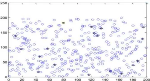
The Fig. 3 shows a random deployment of 400 sensor nodes in 200m 00m area. The sink is located at a corner outside the deployment area. The activity of each node is monitored for each data gathering round and is mapped for the number of transmissions in every round. The activity of each node in one such round, specifically for the deployment shown in Fig. 3, is shown in the activity map 1.

As seen in the Fig. 3, the sink is located at the right corner (200, 250) while the nodes are randomly deployed in an area of

200m200m. While the FCHs (FCH) are many the SCH is only one for this round and is located at (81.78, 188.90). The number of transmissions i.e. sent and received, for every node is analysed and mapped to activity map shown in activity map 1(a) and activity map 1(b) respectively.

Fig. 3. Random deployment of nodes in 200m 00marea (sink outside)

(a) (b)

Activity map 1: Activity of nodes (a) sending transmissions (b) receiving transmissions

As seen in the activity map 1(a), data sending activity is marked all around the map leading to the mapping of moderate transmissions (between 80 and 135) by the sensor nodes at different locations in the map. The two dark patches around (81.78, 188.90) and (22.24, 90.01) signify relatively higher activity. The reason for this high activity around (81.78, 188.90) can be understood from the fact that the proposed HCS allows only the SCHs to communicate with the sink. Since, for this deployment, the SCH is located at (81.78, 188.90) hence it is responsible for sending all the information obtained from its member nodes. This distribution of ability to communicate with the sink allows all the other nodes to save a lot of energy which would have been dissipated by them otherwise. Huge activity is seen around (22.24, 90.01) because the FCH located at this position is the only one in the region and is responsible for sending the data from a large number of nodes. Moderate patches over the map show low number of transmissions (between 80 and 135) between the FCHs and respective SCHs. The sink at the corner shows no activity as it only receives data from the SCH. An important conclusion that can be drawn from this map is that the number of transmissions at every node is moderate and varies between 100 and 150. As seen in the activity maps every node shares the load equally and hence the number of sending activity along with the transmission load on every node is distributed evenly throughout the network.

As seen in the activity map 1(b), data receiving activity is marked all around the map leading to the mapping of moderate transmissions (between 400 and 500) by the sensor nodes at different locations in the map. It must be noticed that moderate receiving activity is seen at all the one hop neighbours and FCHs. The proposed HCS ensures that the number of received transmissions at every node is reduced to a low value (around 400 in this case) except at the SCH. The reduced amount of receiving activity at various FCH shows the advantage of applying CS at the one hop neighbours. The SCH, at (81.78, 188.90), shows the highest number of receiving activity for obvious reasons as it receives data from all the FCHs. As seen in the activity map 1(b), the SCH receives about 1200 transmissions but careful observation reveals that the sink at the corner (200, 250) receives about 300 transmissions only. Comparing the activity maps 1(a) and (b), it becomes clear that although the second level cluster receives a large number of transmissions (in this case about 1200) but with the proposed HCS, the outgoing traffic is reduced to nearly 300. With such a distribution of transmissions, the nodes save a lot of energy and hence the network lifetime is enhanced significantly. A significant deduction from this activity map is that the application of CS at one hop neighbours and at FCHs prevents the nodes from transmitting huge amount of data within the network. Thus, the activity maps proves that with reduced number of transmissions the proposed HCS can enhance the network lifetime significantly.

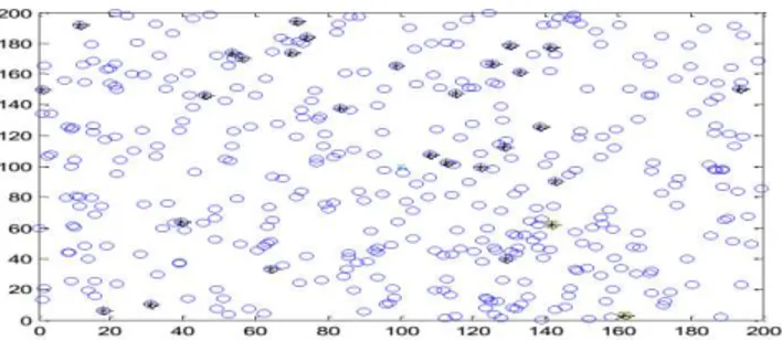
Sink located at the centre

such round, specifically for the deployment shown in Fig. 4, is shown in the activity map 2.

Fig. 4. Random deployment of nodes in 200m 00marea (sink outside)

(a) (b)

Activity map 2: Activity of nodes (a) sending transmissions (b) receiving transmissions

As seen in the activity map 2(a), data sending activity is marked all around the map leading to the mapping of moderate transmissions (between 55 and 110) by the sensor nodes at different locations in the map. The two dark patches around (144.56, 62.76) and (0, 151.01) signify relatively higher activity. The reason for this high activity around (144.56, 62.76) is the presence of SCH. Since the SCH sends majority of the data to the sink, the number of transmissions being sent by the SCH is relatively high (about 300 in this case). A small patch of relatively lower transmissions is seen around (161.08, 2.23) which is the location of the second SCH. The activity at this location is moderate because as seen in the deployment diagram (figure 6) the majority of the FCHs lie closer to (144.56, 62.76) and hence they send their data to it. Thereby leaving only a few FCH to send their data through the SCH at (161.08, 2.23), thus less data to send to the sink. Huge activity is seen around (0, 151.01) because the FCH located at this position is the only one in the region and is responsible for sending the data from a large number of nodes. A patch with moderate activity is seen around (50, 62.7) as there are relatively less number of FCHs in the region and hence increased two hop transmissions. The sink at the centre shows no activity as it only receives data from the SCHs. As compared to the activity map 1(a) the nodes in the activity map 2(a) have lower transmission values ranging between 55 and 110 and the load is more evenly distributed throughout the area. The advantage of having the sink at the centre of the deployment area is the significant reduction in the transmission distance for the SCH. With almost equal activity at every node the load is evenly distributed throughout the area. With sink at the centre the results tend to improve and the effect of this reduction is seen in the lifetime of the network. Another round

of data gathering might result in different number of FCHs and SCHs with different positions.

As seen in the activity map 2(b), data receiving activity is marked all around the map leading to the mapping of moderate transmissions (between 350 and 500) by the sensor nodes at different locations in the map. Important deduction from this activity map is the better distribution of the transmission load as compared to the activity map 1(b) for sink outside the deployment area. The SCH, at (144.56, 62.76), shows the highest number of receiving activity as it receives data from all the majority of the FCHs. As discussed in activity map 2(a) the SCH at (161.08, 2.23) shows relatively low receiving activity as majority FCHs are near to the SCH at (144.56, 62.76). The receiving activity at the sink shows that the number of transmissions received at the sink is almost same as in activity map 1(b) but the difference being the distance between the SCHs and the sink. With sink at the centre, the energy consumption in transmitting the data is relatively low and hence is much better.

C. Transmission Analysis

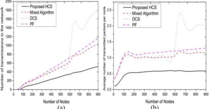
The sink position remaining the same i.e. at the centre, the total number of packets circulating within the network for the proposed HCS is compared with the mixed algorithm proposed in [23]. The performance of the proposed algorithm is also compared with the other approaches i.e. Distributed compressed sensing (DCS) and Pack and forward (PF) strategies as used in [23]. The Fig. 5 shows the behaviour of the proposed HCS and the three existing approaches as the nodes are increased from 9 to 900.

The figure shows a gradual increase in the number of transmissions as the number of nodes is increased. However, Fig. 5 (a) clearly shows that with the proposed HCS, the number of packets within the network is far less as compared to the mixed algorithm proposed in [23] and DCS and PF schemes used for comparison in [23]. Even for a small network, the number of packets in the proposed HCS is much better than the mixed algorithm. Interestingly, a sudden burst, in the number of sent packets, is seen for a particular network size in the mixed algorithm, DCS and PF scheme. However, the proposed HCS remains unaffected with the network size, proving its efficiency over the existing approaches. As seen in Fig. 5 (b), the average number of transmitted packets per node ranges between 0.1175968 and 0.58376 which is much better than the mixed algorithm [23] where the range of per node packet ranges approximately between 0.333856 to 1.1625. The proposed HCS has better performance than the existing approaches, presenting very less number of sent packets which is always better than the mixed algorithm [23], DCS and PF as used in [23].

D. Energy and Network Lifetime analysis

The lifetime of the network is analyzed for both the discussed scenarios. The stability period, first dead and final dead are considered as the parameters for the energy and lifetime analysis.

Sink located outside

(a) (b)

Fig. 5. Comparison among proposed HCS, mixed algorithm, DCS and PF (sink at the centre). (a) Total number of packets circulating within the network. (b) Average number of transmissions per node

Fig. 6. The number of living nodes over rounds (sink outside)

As evident from the Fig. 6, the proposed HCS is able to improve the lifetime of the network to almost 200 % as compared to EEBCDA as proposed in [24]. The first node with the proposed HCS dies in the 1362nd round whereas with EEBCDA [24] the first node dies in the 591st round. The proposed HCS outperforms the EECS [25] and EEBCDA [24], both in terms of stability period and lifetime of the network. The simulations are run until only 10 nodes are alive and, with the proposed scheme, the 390th node dies in the 5380th round after which the network is considered to be dead. An important aspect of EEBCDA [24] and EECS [25] is the even distribution of the load over the network. The relatively small unstable region i.e. the duration between the first and the last dead, in EEBCDA [24] signifies efficient traffic load balancing within the network. However, in the proposed HCS, with sink at the corner outside the deployment area, the SCHs spend huge amount of energy in transmitting their data to the sink. Over the lifetime of the network, every node becomes a SCH and bears this heavy energy consumption. Hence, although the load is distributed efficiently for almost all the nodes in the network, there might be one or more (depending upon the number of SCHs) nodes dissipating huge amount of energy in data transmission to the sink. The presence of such nodes, in every round of data collection, does not allow the proposed HCS to achieve its true potential in terms of stability period and lifetime. The effect is seen in the duration between the first and the last dead of the proposed HCS. After the first node dies in the 1362nd round, the last considered alive node i.e. 390th node dies in the 5380th. Thus, in the current scenario, though the lifetime of the network is improved greatly but the advantage of distributing the load throughout the network is lost.

Changing the position of the sink can not only facilitate the load distribution in the network but can also improve the stability period of the network.

Sink located at the centre

The Fig. 7 shows the lifetime of the proposed HCS with sink at the centre.

Fig. 7. The number of living nodes over rounds (sink at centre)

As evident from the figure, with sink at the centre, not only a perfect distribution of the load is obtained but the stability period is doubled as well. In the current scenario, the first node dies in the 3873rd round whereas when the sink is placed outside the deployment area, the first node dies in the 1362nd round. The proposed HCS, in the current scenario, is able to improve the stability period of the network to almost 200 % as compared to the scheme proposed in scenario 1. The simulations are run until 10 nodes are alive and the 390th node dies in the 5878th round and after this the network is considered to be dead. Comparing the lifetime of EEBCDA proposed in [24] with the proposed HCS (both scenarios), it becomes clear that the proposed HCS (with sink at the centre) improves the lifetime of the network significantly and is able to achieve about 300 % efficiency over EEBCDA [24] and is even better than EECS [25]. With sink at the centre, the proposed HCS is able to efficiently distribute the load throughout the network and hence better traffic load balancing in the network. The effect of this even distribution is seen in the reduced unstable region. Thus, in the current scenario, not only the advantage of distributing the load throughout the network is achieved but the stability period is also improved significantly. Changing the position of the sink to the centre allows the proposed HCS to achieve better results both in terms of network lifetime and reliability as well.

VI. CONCLUSION

improved. The same has been validated through results. The results prove that the proposed HCS outperforms the existing CS based schemes.

VII. FUTURE WORK

We continue to extend our work to analyse the performance of the proposed HCS in a real world deployment. A mathematical model to determine the compression ratio and the communication overhead, remains to be developed in the future.

REFERENCES

[1] Abbasi AA, Younis M. A survey on clustering algorithms for wireless sensor networks. Computer communications. 2007 Oct 15;30(14):2826-41.

[2] Singh S, Chand S, Kumar B. Energy Efficient Clustering Protocol Using Fuzzy Logic for Heterogeneous WSNs. Wireless Personal Communications. 2016 Jan 1;86(2):451-75.

[3] Xue Y, Cui Y, Nahrstedt K. Maximizing lifetime for data aggregation in wireless sensor networks. Mobile Networks and Applications. 2005 Dec 1;10(6):853-64.

[4] Tan HÖ, Körpeoǧlu I. Power efficient data gathering and aggregation in

wireless sensor networks. ACM Sigmod Record. 2003 Dec 1;32(4):66-71.

[5] Sinha A, Lobiyal DK. A multi-level strategy for energy efficient data aggregation in wireless sensor networks. Wireless personal communications. 2013 Sep 1;72(2):1513-31.

[6] Banerjee T, Chowdhury KR, Agrawal DP. Using polynomial regression for data representation in wireless sensor networks. International Journal of Communication Systems. 2007 Jul 1;20(7):829-56.

[7] Othman SB, Bahattab AA, Trad A, Youssef H. Confidentiality and Integrity for Data Aggregation in WSN Using Homomorphic Encryption. Wireless Personal Communications. 2015 Jan 1;80(2):867-89.

[8] Liu T, Li Q, Liang P. An energy-balancing clustering approach for gradient-based routing in wireless sensor networks. Computer Communications. 2012 Oct 1;35(17):2150-61.

[9] Sutagundar AV, Manvi SS. Wheel based Event Triggered data aggregation and routing in Wireless Sensor Networks: Agent based approach. Wireless Personal Communications. 2013 Jul 1;71(1):491-517.

[10] Khedo K, Doomun R, Aucharuz S. Reada: Redundancy elimination for accurate data aggregation in wireless sensor networks. Wireless Sensor Network. 2010 Apr 1;2(4):300.

[11] Guo W, Xiong N, Vasilakos AV, Chen G, Cheng H. Multi-source temporal data aggregation in wireless sensor networks. Wireless personal communications. 2011 Feb 1;56(3):359-70.

[12] Enachescu M, Goel A, Govindan R, Motwani R. Scale free aggregation in sensor networks. InAlgorithmic Aspects of Wireless Sensor Networks 2004 Jul 16 (pp. 71-84). Springer Berlin Heidelberg.

[13] Luo J, Xiang L, Rosenberg C. Does compressed sensing improve the throughput of wireless sensor networks?. InCommunications (ICC), 2010 IEEE International Conference on 2010 May 23 (pp. 1-6). IEEE.

[14] Razzaque MA, Dobson S. Energy-efficient sensing in wireless sensor networks using compressed sensing. Sensors. 2014 Feb 12;14(2):2822-59.

[15] Xiang L, Luo J, Vasilakos A. Compressed data aggregation for energy efficient wireless sensor networks. InSensor, mesh and ad hoc communications and networks (SECON), 2011 8th annual IEEE communications society conference on 2011 Jun 27 (pp. 46-54). IEEE. [16] Caione C, Brunelli D, Benini L. Compressive sensing optimization over

ZigBee networks. InSIES 2010 Jul 7 (pp. 36-44).

[17] Mehrjoo S, Shanbehzadeh J, Pedram MM. A novel intelligent energy-efficient delay-aware routing in wsn, based on compressive sensing. InTelecommunications (IST), 2010 5th International Symposium on 2010 Dec 4 (pp. 415-420). IEEE.

[18] Zheng H, Xiao S, Wang X, Tian X. On the capacity and delay of data gathering with compressive sensing in wireless sensor networks. InGlobal Telecommunications Conference (GLOBECOM 2011), 2011 IEEE 2011 Dec 5 (pp. 1-5). IEEE.

[19] Zheng H, Xiao S, Wang X, Tian X, Guizani M. Capacity and delay analysis for data gathering with compressive sensing in wireless sensor networks. Wireless Communications, IEEE Transactions on. 2013 Feb;12(2):917-27.

[20] Xu X, Ansari R, Khokhar A. Power-efficient hierarchical data aggregation using compressive sensing in WSNs. InCommunications (ICC), 2013 IEEE International Conference on 2013 Jun 9 (pp. 1769-1773). IEEE.

[21] Chung WY, Villaverde JF. Implementation of Compressive Sensing Algorithm for Wireless Sensor Network Energy Conservation. InInternational Electronic Conference on Sensors and Applications 2014. Multidisciplinary Digital Publishing Institute.

[22] Qaisar S, Bilal RM, Iqbal W, Naureen M, Lee S. Compressive sensing: From theory to applications, a survey. Communications and Networks, Journal of. 2013 Oct;15(5):443-56.

[23] Caione C, Brunelli D, Benini L. Distributed compressive sampling for lifetime optimization in dense wireless sensor networks. Industrial Informatics, IEEE Transactions on. 2012 Feb;8(1):30-40.

[24] Yuea J, Zhang W, Xiao W, Tang D, Tang J. Energy efficient and balanced cluster-based data aggregation algorithm for wireless sensor networks. Procedia Engineering. 2012 Dec 31;29:2009-15.

[25] Ye M, Li C, Chen G, Wu J. EECS: an energy efficient clustering scheme in wireless sensor networks. InPerformance, Computing, and Communications Conference, 2005. IPCCC 2005. 24th IEEE International 2005 Apr 7 (pp. 535-540). IEEE.

[26] Chand S, Singh S, Kumar B. Heterogeneous HEED protocol for wireless sensor networks. Wireless personal communications. 2014 Aug 1;77(3):2117-39.

[27] Davenport MA, Duarte MF, Eldar YC, Kutyniok G. Introduction to compressed sensing. Preprint. 2011;93(1):2.

[28] Han Z, Li H, Yin W. Compressive sensing for wireless networks. Cambridge University Press; 2013 Jun 6.

[29] Razzaque MA, Bleakley C, Dobson S. Compression in wireless sensor networks: A survey and comparative evaluation. ACM Transactions on Sensor Networks (TOSN). 2013 Nov 1;10(1):5.