Model Development for Risk Assessment of Driving on Freeway under Rainy Weather Conditions.

Model Development for Risk Assessment of

Driving on Freeway under Rainy Weather

Conditions

Xiaonan Cai1, Chen Wang2*, Shengdi Chen3, Jian Lu1,2

1Transportation Research Center, School of Naval Architecture, Ocean and Civil Engineering, Shanghai Jiao Tong University, Shanghai, P.R. China,2School of Transportation Engineering, Tongji University, Shanghai, P.R. China,3College of Transport and Communications, Shanghai Maritime University, Shanghai, P.R. China

*[email protected]

Abstract

Rainy weather conditions could result in significantly negative impacts on driving on free-ways. However, due to lack of enough historical data and monitoring facilities, many regions are not able to establish reliable risk assessment models to identify such impacts. Given the situation, this paper provides an alternative solution where the procedure of risk assess-ment is developed based on drivers’subjective questionnaire and its performance is vali-dated by using actual crash data. First, an ordered logit model was developed, based on questionnaire data collected from Freeway G15 in China, to estimate the relationship between drivers’perceived risk and factors, including vehicle type, rain intensity, traffic vol-ume, and location. Then, weighted driving risk for different conditions was obtained by the model, and further divided into four levels of early warning (specified by colors) using a rank order cluster analysis. After that, a risk matrix was established to determine which warning color should be disseminated to drivers, given a specific condition. Finally, to validate the proposed procedure, actual crash data from Freeway G15 were compared with the safety prediction based on the risk matrix. The results show that the risk matrix obtained in the study is able to predict driving risk consistent with actual safety implications, under rainy weather conditions.

Introduction

Weather affects driver capabilities, vehicle performance, pavement friction, roadway infra-structure, and crash risk through visibility impairments, precipitation, high winds, and temper-ature extremes. According to the National Highway Traffic Safety Administration in the United States, from 2002 to 2012, there were on average 1,311,970 weather-related crashes each year, resulting in 480,338 injuries and 6,253 deaths and the vast majority of weather-related crashes happened on wet pavements (74%) and during rainfall (46%) [1]. Similarly in China, based on an annual report of road accidents statistics, there were about 56,809 weather-related crashes in 2012, resulting in 65,243 injuries and 17,040 deaths and over forty percent of these crashes occurred under rainy weather conditions [2]. Whether it is in the United State or OPEN ACCESS

Citation:Cai X, Wang C, Chen S, Lu J (2016) Model Development for Risk Assessment of Driving on Freeway under Rainy Weather Conditions. PLoS ONE 11(2): e0149442. doi:10.1371/journal. pone.0149442

Editor:Xiaosong Hu, Chongqing University, CHINA

Received:November 26, 2015

Accepted:February 1, 2016

Published:February 19, 2016

Copyright:© 2016 Cai et al. This is an open access article distributed under the terms of theCreative Commons Attribution License, which permits unrestricted use, distribution, and reproduction in any medium, provided the original author and source are credited.

Data Availability Statement:Data are available from the Transportation Research Center in Shanghai Jiao Tong University for researchers who meet the criteria for access to confidential data. In addition, the minimal data set underlying the findings in our study has been uploaded in the supplemental files.

China, rainy weather has significantly negative impacts on driving safety. Therefore, it could be necessary to develop travel weather warning systems (TWWS) to help drivers identifying driv-ing risk on rainy days.

Road Weather Information System (RWIS) as a kind of TWWS has been successfully applied for aiding decision-making of highway administrations in Europe and America. This system can collect and monitor real-time traffic and weather conditions, and disseminate early warning information to drivers. The cores of the RWIS are their risk estimate models, which were developed based on large weather-related crash data. However, most developing countries are unable to establish their own TWWS due to the lack of sufficient and reliable weather-related crash data. For example, in China, there is only one meteorological criterion [3] used for road weather management instead of the professional TWWS, and the criterion only con-siders weather parameters and ignores significant impacts of traffic conditions such as vehicle type and traffic volume.

To fill the gap, this paper attempts to develop a procedure of risk assessment used to evalu-ate driving risk on rainy days. And the procedure should include combined impacts of multiple factors instead of only meteorological factors and not depend much on historical weather-related crash data.

Literature Review

Generally, there are three types of research methods on evaluating rain-related driving risks. Firstly, their engineering aspects are well understood. In particular, the physical effects of rain on pavement friction [4,5] and driver visibility [6,7] were given much attention. However, con-verting estimates of frictional change or impaired visibility into driving risk is much more diffi-cult considering the stochastic nature of crashes.

Secondly, many traffic safety research activities related to rainy weather focus on analyzing accidents. Palutikof found that rainy weather was the most significant one among all weather factors which resulted in traffic fatalities [8]. In a study by Sherretz and Farhar, it was found that there existed a linear positive correlation between rainfall and traffic crash frequency [9]. More detailed findings about impacts of rainy weather on traffic safety were summarized by Andrey et al. [10] and Eisenberg [11]. However, few researches in developing countries (e.g. China) have been identified due to lack of rain-related crash data.

Thirdly, risk perceptions by drivers are used to identify rain-related driving risks. Andrey and Knapper found that drivers did recognize the evaluated risk associated with adverse weather conditions [12]. Some studies showed that drivers’subjective assessments of the rela-tive danger associated with driving during various weather scenarios were reasonably consis-tent with collision studies [12,13]. That is to say, subjective data from drivers could be applied for evaluating driving risk on rainy days. Driving inexperience is one of the key predictors of crash rates [14], with young novice drivers being at risk particularly [15]. Furthermore, the higher accident rate of young drivers is due to their poor cognitive skills [16] and inattention [17]. On the contrary, experienced drivers can adapt their strategies in time by anticipating var-ious demands of different driving conditions [18]. In light of these, if driving perception by experienced drivers could be provided to young novice drivers, it could be expected that they would better identify driving risk on rainy days and lower crash potential.

Risk assessment is a scientific process of evaluating adverse effects caused by a substance, activity, lifestyle, or natural phenomenon [19]. According to Berdica, the definition of accident risk consisted of two parts: the probability of accident occurrence and the consequence [20]. Some studies [21] considered Relative Risk Ratio (RRR) as an effective method to quantify crash risk under adverse weather conditions. But the method requires a large number of

weather-related accident records to match pairs. Another alternative method is using a risk matrix [20], which includes combined effects of consequence and probability.

The study summarized in this paper attempts to develop a procedure for risk assessment of driving on the freeway under rainy weather conditions, which is based on drivers’risk percep-tion. Data were derived from drivers’subjective questionnaire and actual traffic crashes on China National Freeway G15 (with kilometer post: k1184+275~k1215+870). A risk matrix with the combined effects of consequence and probability was established to determine levels of driving risk. Furthermore, actual crash data on the same freeway segment from May in 2008 to June in 2011 were used to examine the validity of the risk matrix. Being warned by the level of driving risk, drivers, especially young novice drivers, could better identify surrounding risk.

Methods

The study was approved by the Ethics Committee of Shanghai Jiao Tong University. The data derived from drivers’questionnaire drafted by Dr. Xiaonan Cai was analyzed anonymously and therefore no additional informed consent was required. In addition, Dr. Xiaonan Cai and other researchers in Transportation Research Center including Chen Wang, and Jian Lu administered this questionnaire. Moreover, the details about the questionnaire can be seen in the section of Data.

Ordered logit models and rank order cluster analysis are the two main mathematical models in this study. The former was used to calculate impacts and corresponding probabilities associ-ated with various driving circumstances on rainy days. The latter was employed for driving risk classification.

Ordered Logit Model

The dependent variable, level of impact on driving (Ci), is considered discrete in the modeling

withCiranged from slight impact, general impact, serious impact, and catastrophic impact,

andirepresenting theithdriver. Observable independent variables include vehicle type, rain intensity, traffic volume, and location. As a general practice, a non-observable variableε_iis assumed to fit a logistic distribution in order to calculate a continuous latent variableCi

, which is called as impact on driving, or

Ci ¼

XJ

j

xijbjþεi; Ci ¼1;2;. . .;M ð1Þ

where,Jis number of observable independent variables,Mis number of dependent variable,β_j

is the coefficient for thejthvariable, and the dependent variableCihas the following

relation-ship with the latent variableCi

:

Ci ¼

1 _{if C}

i c1

2 _{if c}

1<C i c2

3 _{if c}

2<C i c3

. . . . . .

M if cM 1<C

i

ð2Þ

8 > > > > > > > > < > > > > > > > > :

where,ck(k= 1, 2,. . .,M-1) are threshold values to satisfy:c1<c2<. . .<cM-1. As mentioned

Thus, probabilities of different levels of impact can be calculated as follows:

PðCi¼1Þ ¼

expc1

X xijbj

1_þexp

c1

X xijbj

PðCi¼2Þ ¼

expc2

X xijbj

1_þexpc

2

X xijbj

expc1

X xijbj

1_þexpc

1

X xijbj

. . . .

PðCi¼MÞ ¼1

expcM 1

X xijbj

1_þexpc

M 1

X xijbj

ð3Þ

8 > > > > > > > > > > > > > > > > > < > > > > > > > > > > > > > > > > > :

By definition, driving risk (Ri) represents impact on driving (Ci

) multiplied by the corre-sponding probability (Pi). Consequently, a series ofRican be calculated to measure driving risk

on rainy days.

Rank Order Cluster Analysis

It is assumed that driving risk (Ri) could be obtained and sorted by the ascending order, as

indi-cated byR(1),R(2),. . .,R(n). A certain category (G), includingR(i),R(i+1),. . .,R(j)and satisfying

j>i, can be expressed as G = {i,i+1,. . ._{,j}. On the basis, the diameter ofG,D(i,j), is calculated}

as follows:

Dði;jÞ ¼X

j

t¼i

ðRðtÞ RGÞ 2

ð4Þ

where,RGis the mean value of driving risk in the categoryG.

When driving risk is divided intokcategories, different categories are expressed as follows:

G1 ¼ fi1;i1þ1;. . .;i2 1g

G2 ¼ fi2;i2þ1;. . .;i3 1g

. . . .

Gk ¼ fik;ikþ1;. . .;ikþ1 1g

ð5Þ

8 > > > > < > > > > :

where,iis to satisfy 1 =i1<i2<. . .<ik<ik+1= n+1.

The loss function is defined by the formula (6), which represents the sum of diameters fork

categories. Whennandkare given, the smaller the loss function is, the better the classification of driving risk is. Then the minimal loss function has a recursion relationship shown in the for-mula (7).

L½bðn;kފ ¼X

k

t¼1

Dðit;itþ1 1Þ ð6Þ

L½Pðn;2_{ފ ¼min}

2jnfDð1;j 1Þ þDðj;nÞg

L½Pðn;kފ ¼minkjnfL½Pðj 1;k 1ފ þDðj;nÞg

ð7Þ

(

In this study, driving risk is classified into four categories (k= 4). Thus, the optimal catego-ries of driving risk can be determined as the following method. Firstly,j4that minimizes the

formula (8) should be found. Then, the fourth category is expressed asG4= {j4,j4+1,. . .,n}.

L½Pðn;4_{ފ ¼L½Pðj}

4 1;3ފ þDðj4;nÞ ð8Þ

Secondly,j3should be found, satisfying the formula (9). Then, the third category is

expressed asG3= {j3,j3+1,. . .,j4-1}.

L½Pðj4 1;3ފ ¼L½Pðj3 1;2ފ þDðj3;j4 1Þ ð9Þ

The rest of categories can be found in the same manner. Therefore, {G1,G2,G3,G4,} are the

optimal categories of driving risk.

Data

Questionnaire Design

The segment of National Freeway G15 is located between Suzhou city and Nantong city in Jiangsu Province, with about 32 km in length and a six-lane in both directions. And a general view of the segment is shown inFig 1. Since the segment opened to traffic for only a few years, it could not accumulate enough crash data to be used for risk assessment of driving on rainy days. And crash data derived from other similar freeways in China could not be obtained, given possibly political impacts. Thus, a questionnaire to drivers was designed for collecting drivers’risk perception on rainy days. In addition, some crash records collected from the seg-ment were used to validate the proposed procedure of risk assessseg-ment.

The questionnaire survey collects information of driver, vehicle, rain intensity, and traffic condition. In order to help drivers better understand the survey, some explanations have been noted. First, according to the national specification JTG B01-2003 [22], two-axle large trucks and multi-axle large trucks are combined into a category of large vehicles. Thus, vehicle type only consists of small vehicles (including middle-size vehicles) and large vehicles.

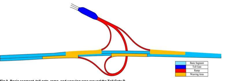
Second, the freeway segment is divided into four parts, including basic segments, toll gates, ramps, and weaving areas. For example, as shown inFig 2, the four parts around the Toll Gate D are labeled by four different colors. Specifically, the toll gate is the segment between two change points of roadway width around the Toll Gate D; the weaving areas indicate the seg-ments that are 500 meters from converging or diverging points on the mainline; the ramps are the connecting segments between the toll gate and the weaving areas; the basic segments are the remaining segments except for the weaving areas on the mainline.

Third, the category descriptions of rain intensity and traffic volume are summarized in Table 1. In the group of rain intensity, the visibility is categorized into four levels based on the specification QX/T 111–2010 [3] and the definitions of light rain, moderate rain, heavy rain and rain storm in this study are consistent with those in the weather forecast, which are easier for drivers to understand. In addition, the traffic volume is categorized into four levels based

Fig 1. A general view of the segment of National Freeway G15 (Kilometer post: k1184+275~k1215 +870).

on the specification JTG B01-2003 [22]. For the freeway segment, actual volume data had been being monitored and collected by the G15 Highway Management System (HMS) from May in 2008 to June in 2011. Furthermore, inTable 1,Vindicates actual data of hourly volume in one direction when the questionnaire survey is made, andCindicates the maximum of hourly vol-ume in one direction from May in 2008 to June in 2011.

Data Collection

Questionnaire surveys were prepared to acquire the data of drivers’demographic information and risk perceptions. Demographic information included age, gender, the type of vehicle driven, and driving experience. Drivers were asked to identify the risks (i.e. impacts) of differ-ent driving conditions on a four-point scale (slight, general, serious, catastrophic).

Surveys were conducted at sites including Toll Gate B, Toll Gate E and a service area around Toll Gate B inFig 1. The duration of surveys was about three months from April to June in 2012 during which rainy weather were expected. With the help of law enforcement officials, respondents were randomly selected according to the last digit of their license plates. Mean-while, one-on-one questionnaire surveys were employed from 7:00 a.m. to 11:00 a.m. and from 2:00 p.m. to 6:00 p.m. Each questionnaire took about 13 minutes on average. The total number of questionnaires received in this survey was 1694, and the number of effective questionnaires Fig 2. Basic segment, toll gate, ramp, and weaving area around the Toll Gate D.

doi:10.1371/journal.pone.0149442.g002

Table 1. Category descriptions of rain intensity and traffic volume. Levels of Rain Intensity

Levels Descriptions

I visibility about 500 meters, light rain

II visibility about 200 meters, moderate rain

III visibility about 100 meters, heavy rain

IV visibility less than 50 meters, rain storm

Levels of Traffic Volume

Levels V/C

I 0.00~0.31

II 0.31~0.67

III 0.67~0.86

IV 0.86~1.00

(driving experience more than two year, no illegal crash records in the past year and the num-ber of trips on the freeway each month not less than two) among them was 1216.

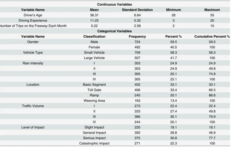
The descriptive statistics of the main variables derived from drivers’questionnaires and actual volume data are summarized inTable 2. In addition, a crosstab of rain intensity and impact on driving was developed. The coefficients of Spearman correlation and Fisher’s exact test were calculated, which is equal to 0.675 and 797.374 (sig.<0.05), respectively, indicating a significantly positive relationship between them.

Results

Assumptions

The study assumes that perceived risk by drivers is consistent with actual crash statistics in evaluating driving risk under rainy weather conditions. Past studies show that drivers’ subjec-tive assessment of relasubjec-tive dangerousness associated with driving during various weather sce-narios are reasonably consistent with collision-based studies [12,13]. But it is undeniable that risk perception could be subject to variation among drivers and regions. Thus, crash data on rainy days were used to validate whether the procedure of risk assessment based on drivers’

risk perception was feasible (in section of Crash Data Validation). Table 2. Descriptive statistics of the main variables.

Continuous Variables

Variable Name Mean Standard Deviation Minimum Maximum

Driver’s Age 36.31 6.64 26 55

Driving Experience 11.25 5.32 3 20

Number of Trips on the Freeway Each Month 5.22 2.58 2 10

Categorical Variables

Variable Name Classification Frequency Percent % Cumulative Percent %

Gender Male 724 59.5 59.5

Female 492 40.5 100

Vehicle Type Small Vehicle 709 58.3 58.3

Large Vehicle 507 41.7 100

Rain Intensity I 303 24.9 24.9

II 303 24.9 49.8

III 305 25.1 74.9

IV 305 25.1 100

Location Basic Segment 402 33.1 33.1

Toll Gate 406 33.4 66.5

Ramp 245 20.1 86.6

Weaving Area 163 13.4 100

Traffic Volume I 273 22.4 22.4

II 333 27.4 49.8

III 366 30.1 79.9

IV 244 20.1 100

Level of Impact Slight Impact 220 18.1 18.1

General Impact 350 28.8 46.9

Serious Impact 375 30.8 77.7

Catastrophic Impact 271 22.3 100

The Ordered Logit Model

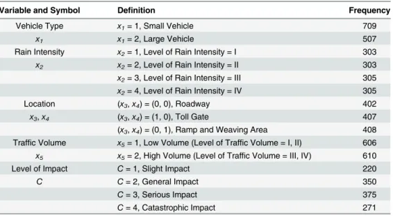
The study specifies four important factors from the survey, including vehicle type, rain inten-sity, traffic volume, and location. Symbols and definitions of the variables are listed inTable 3. Among them, three factors, except location, are defined as ordinal variables. The factor of loca-tion is considered as a nominal variable with four categories, and defined as three dummy vari-ables (0, 1). With the initial variable settings, the first ordered logit model used for risk

assessment is not well fitted, for the variables of“traffic volume”and“location on the freeway”

are not significant at the degree of confidence of 0.95 (AIC = 1318.541, SC = 1357.790). There-fore, some adjustments on independent variables should be made (the second model with smaller AIC and SC values associated with the first model, see inTable 4. First,“traffic volume”

is redefined to have two categories (i.e. low volume and high volume). Second, for“location on the freeway”, ramp and weaving area are combined into one category. That is,“location on the freeway”is defined as two dummy variables.

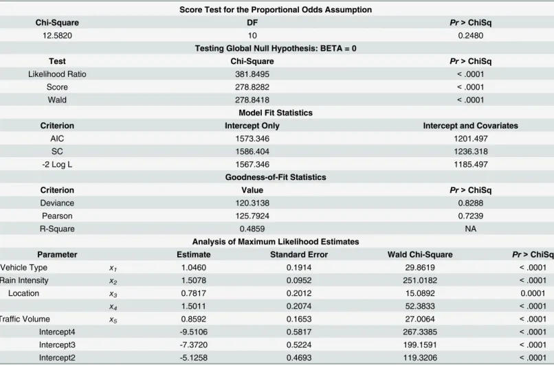
The second ordered logit model was estimated using SAS software and model results are listed inTable 4. Firstly, thePrvalue of score test for the proportional odds assumption is equal to 0.2480, meaning the null hypothesis (i.e. the ordered logit coefficients are equal across the levels of the outcome) could not be rejected. Secondly,Prvalues of statistics of testing global null hypothesis are less than 0.05, meaning there is at least one that could not be equal to zero among all ordered logit coefficients. Thirdly, in term of model fit statistics, criterion AIC and SC provide a means for model selection and promising models give small values for these criteria. Finally, the R-square of the model is equal to 0.4859. With linear regression different, when R-square val-ues of ordered logit models are more than 0.3, the models would be considered to a well fit.

In addition, considering association of predicted probabilities and observed responses, the percent of concordant pairs is equal to 81.3% andcstatistic is equal to 0.827. In conclusion, the ordered logit model has good quality to describe drivers’risk perception of driving on the free-way under rainy weather conditions.

Meanwhile, coefficients of independent variables and model intercepts were estimated using maximum likelihood values. As presented inTable 4, each independent variable is statistically significant and has a positive relationship with the dependent variable (i.e. level of impact). Table 3. Symbols and definitions of variables in the ordered logit model.

Variable and Symbol Definition Frequency

Vehicle Type x1= 1, Small Vehicle 709

x1 x1= 2, Large Vehicle 507

Rain Intensity x2= 1, Level of Rain Intensity = I 303

x2 x2= 2, Level of Rain Intensity = II 303

x2= 3, Level of Rain Intensity = III 305

x2= 4, Level of Rain Intensity = IV 305

Location (x3,x4) = (0, 0), Roadway 402

x3,x4 (x3,x4) = (1, 0), Toll Gate 407

(x3,x4) = (0, 1), Ramp and Weaving Area 408

Traffic Volume x5= 1, Low Volume (Level of Traffic Volume = I, II) 606

x5 x5= 2, High Volume (Level of Traffic Volume = III, IV) 610

Level of Impact C= 1, Slight Impact 220

C C= 2, General Impact 350

C= 3, Serious Impact 375

C= 4, Catastrophic Impact 271

Impact (C) and level of impact (C) have a following relationship with all parameters (vari-ables) specified inTable 4:

C_¼1:0460x

1þ1:5078x2þ0:7817x3þ1:5011x4þ0:8592x5

C¼

1 _{if C5:1258}

2 _if 5_:1258_{<C 7:3720}

3 _if 7_:3720_{<C 9:5106}

4 _if 9_:5106_<C

ð10Þ

8 > > > > > > > < > > > > > > > :

As a consequence, the probabilities (Pi) of four levels of impact (Ci) could be calculated as

follows:

logitðP4Þ ¼ 9:5106þ1:0460x1þ1:5078x2þ0:7817x3þ1:5011x4þ0:8592x5

logitðP3þP4Þ ¼ 7:3720þ1:0460x1þ1:5078x2þ0:7817x3þ1:5011x4þ0:8592x5

logitðP2þP3þP4Þ ¼ 5:1258þ1:0460x1þ1:5078x2þ0:7817x3þ1:5011x4þ0:8592x5

P1¼1 ðP2þP3þP4Þ

ð11Þ

8 > > > > < > > > > :

Table 4. Results of the ordered logit model.

Score Test for the Proportional Odds Assumption

Chi-Square DF Pr_>ChiSq

12.5820 10 0.2480

Testing Global Null Hypothesis: BETA = 0

Test Chi-Square Pr_>ChiSq

Likelihood Ratio 381.8495 <.0001

Score 278.8282 <_.0001

Wald 278.8418 <_.0001

Model Fit Statistics

Criterion Intercept Only Intercept and Covariates

AIC 1573.346 1201.497

SC 1586.404 1236.318

-2 Log L 1567.346 1185.497

Goodness-of-Fit Statistics

Criterion Value Pr_>ChiSq

Deviance 120.3138 0.8288

Pearson 125.7924 0.7239

R-Square 0.4859 NA

Analysis of Maximum Likelihood Estimates

Parameter Estimate Standard Error Wald Chi-Square Pr_>ChiSq

Vehicle Type x1 1.0460 0.1914 29.8619 <.0001

Rain Intensity x2 1.5078 0.0952 251.0182 <.0001

Location x3 0.7817 0.2012 15.0892 0.0001

x4 1.5011 0.2074 52.3833 <.0001

Traffic Volume x5 0.8592 0.1653 27.0064 <.0001

Intercept4 -9.5106 0.5817 267.3385 <.0001

Intercept3 -7.3720 0.5224 199.1591 <_.0001

Intercept2 -5.1258 0.4693 119.3206 <_.0001

where,P1,P2,P3,P4is the probability of slight impact, general impact, serious impact, and

cata-strophic impact, respectively.

Weighted Driving Risk

By definition, driving risk (R) equals impact on driving (C) multiplied by the corresponding probability (P). However, it should be noted that the definition of driving risk literally com-mensurate adverse events of high impacts and low probabilities with events of low impacts and high probabilities. An effective solution for such a problem is to assign a weight variable to each individual level of impact. Thus, weighted driving risk (WR) can be expressed as follows:

WR¼CPW¼ ð1_:0460_x

1þ1:5078x2þ0:7817x3þ1:5011x4þ0:8592x5Þ PW ð12Þ

where,PandWare the probabilities and the weights for four levels of impact, respectively. The weight variable was determined by Delphi method with focus group discussions. Ten members with experience and expertise in traffic safety and operations joined the discussions. The average values of weights from the ten experts for each level of impact are used as the final weights, which are equal to 0.6, 0.9, 1.2, and 1.5 for slight impact, general impact, serious impact, and catastrophic impact, respectively. Based on the formula (12), a series ofWRcan be calculated and the larger theWRvalue, the higher perceived risk by drivers. In other words, according to theWRvalues, driving risk under various conditions can be measured and com-pared. However,WRis only a relative measure of driving risk without any physical implica-tions, which is not easily understood by drivers and road weather managers. Thus, theseWR

values should be classified into different levels of early warning. In addition, sensitivity analysis of weights is presented in section of Discussions.

The Rank Order Cluster Analysis

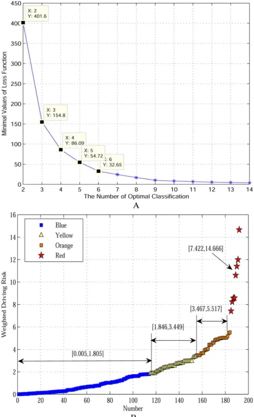
As stated previously, this study classified weighted driving risk (WR) using the rank order clus-ter analysis. Firstly, theWRvalues were sorted by the ascending order. Secondly, the minimal loss functions for different categories were calculated by the MATLAB programming and the results show that the minimal loss functions decrease with number of classifications increasing inFig 3A. In China, an early warning system normally has four different warning colors. Accordingly, theWRwas classified into four levels (k= 4) and the corresponding loss function was equal to 86.09. Finally, the optimal classification ofWRwas found and the four levels of

WRwere coded as blue, yellow, orange, and red, with red color representing the highest risk. Furthermore, the corresponding ranges for four warning colors are shown inFig 3B. That is, when aWRvalue lies in the range from 0.005 to 1.805, a blue early warning is disseminated. However, such method used for early warning could be too complex in real practice. A feasible way is to establish a risk matrix with combined effects of impact and probability.

Risk Matrix

Fig 3. Results of the rank order cluster analysis through MATLAB programming.Panel A shows minimal loss functions vary with number of classifications. Panel B shows distribution ranges of four levels of weighted driving risk (k = 4).

Fig 4. Conducting the risk matrix of driving on freeway under rainy weather conditions.Panel A shows distribution of early warning colors of weighted driving risk.Panel B shows risk matrix with combined effects of impact and probability.

Crash Data Validation

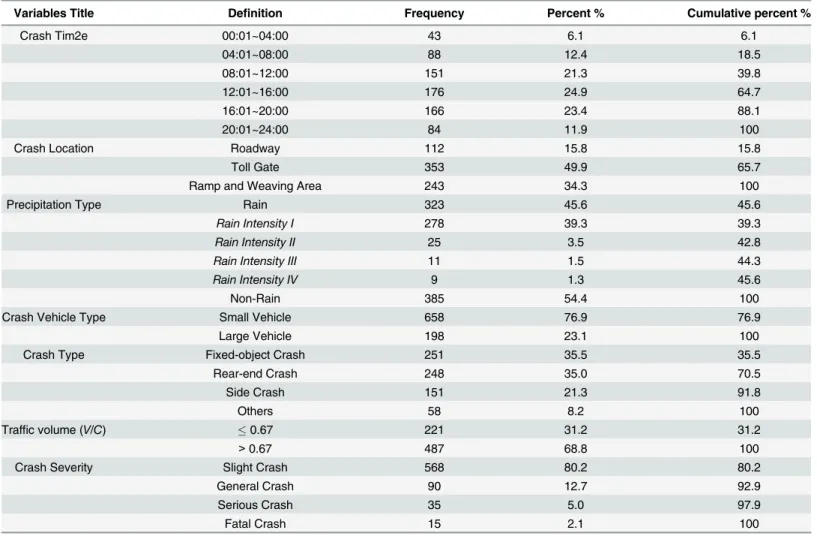
To validate the proposed risk matrix, 708 crashes derived from the segment of National Free-way G15 (K1184+275~K1215+870) were collected from May in 2008 to June in 2011. Crash data from the segment are available with specific information related to crash characteristics, meteorological elements and traffic conditions. Crash severity was divided into four categories: slight crash, general crash, serious crash, and fatal crash with the definitions based on: (1) dam-age to traffic facilities, (2) injury to occupant, (3) occupancy to lane. Crash descriptions are listed inTable 5.

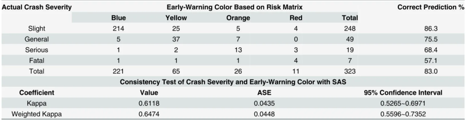
By inputting actual data including crash location, crash vehicle type, rain intensity, and traf-fic volume into the ordered logit model (formula10and11), early-warning colors can be deter-mined by the risk matrix approach and compared with actual crash severity to validate

whether the procedure of risk assessment summarized in the study is feasible. The comparison results are listed inTable 6. Among 323 crashes occurring on rainy days, totally 268 crashes are correctly predicted their warning colors, and the percentage of the correct prediction for slight, general, serious, and fatal crashes is 86.3%, 75.5%, 68.4% and 57.1%, respectively. The predic-tion accuracy for fatal crashes is relatively low. This could be due to the limited sample size. Moreover, Kappa and Weighted Kappa coefficients are calculated to test the consistency between early-warning colors and actual crash severities. As shown inTable 6, the two

Table 5. Descriptions of crashes from the segment of National Freeway G15.

Variables Title Definition Frequency Percent % Cumulative percent %

Crash Tim2e 00:01~04:00 43 6.1 6.1

04:01~08:00 88 12.4 18.5

08:01~12:00 151 21.3 39.8

12:01~16:00 176 24.9 64.7

16:01~20:00 166 23.4 88.1

20:01~24:00 84 11.9 100

Crash Location Roadway 112 15.8 15.8

Toll Gate 353 49.9 65.7

Ramp and Weaving Area 243 34.3 100

Precipitation Type Rain 323 45.6 45.6

Rain Intensity I 278 39.3 39.3

Rain Intensity II 25 3.5 42.8

Rain Intensity III 11 1.5 44.3

Rain Intensity IV 9 1.3 45.6

Non-Rain 385 54.4 100

Crash Vehicle Type Small Vehicle 658 76.9 76.9

Large Vehicle 198 23.1 100

Crash Type Fixed-object Crash 251 35.5 35.5

Rear-end Crash 248 35.0 70.5

Side Crash 151 21.3 91.8

Others 58 8.2 100

Traffic volume (V/C) 0.67 221 31.2 31.2

>0.67 487 68.8 100

Crash Severity Slight Crash 568 80.2 80.2

General Crash 90 12.7 92.9

Serious Crash 35 5.0 97.9

Fatal Crash 15 2.1 100

coefficients are both more than 0.6. Landis and Koch gave an interpretation of the range of Kappa coefficients: [0.6~0.8], Substantial; [0.8~1], almost perfect [23]. Considering stochastic nature of traffic accidents, the consistency between the two is fairly good and the proposed pro-cedure in the study is able to capture actual risk implication on the freeway on rainy days.

Discussions

Sensitivity Analysis of Weights

A sensitivity analysis of weights was conducted to identify how early warning colors would change with weights. The original settings of weights were 0.6, 0.9, 1.2, and 1.5, for slight, gen-eral, serious and catastrophic impact, respectively. When the weights vary, the corresponding early warning colors could change. To identify such potential impact, Kappa and Weighted Kappa coefficients were calculated. As listed inTable 7, the two coefficients are much higher than 0.8. In other words, variations in the four weights will not lead to great change of early warning colors.

Limitations

Some studies indicate that risk perception could be impacted by driver age, gender, driving experience, and accident history. However, the procedure of risk assessment summarized in the study did not analyze effects of these factors on driving risk on rainy days. Instead, these factors were considered as non-observable variables and assumed to fit a logistic distribution in the ordered logit model.

Without any doubts, the relationships among driver’s perception, behavior and actual crashes are so intricate and complicated. Even if drivers have correct perceptions of driving risk, different drivers might take various actions, resulting in different consequences. However, at least, for inexperienced drivers, this procedure could help them better identify driving risk, Table 6. Comparisons of early-warning color and actual crash severity.

Actual Crash Severity Early-Warning Color Based on Risk Matrix Correct Prediction %

Blue Yellow Orange Red Total

Slight 214 25 5 4 248 86.3

General 5 37 7 0 49 75.5

Serious 1 2 13 3 19 68.4

Fatal 1 1 1 4 7 57.1

Total 221 65 26 11 323 83.0

Consistency Test of Crash Severity and Early-Warning Color with SAS

Coefficient Value ASE 95% Confidence Interval

Kappa 0.6118 0.0435 0.5265~0.6971

Weighted Kappa 0.6474 0.0448 0.5596~0.7352

doi:10.1371/journal.pone.0149442.t006

Table 7. Sensitivity analysis of four subjective weights with SAS.

Variation Weights Setting Kappa Coefficient 95% Confidence Interval Weighted Kappa Coefficient 95% Confidence Interval

-0.2 (0.4, 0.7, 1.0, 1.3) 0.9596 (0.9249,0.9943) 0.9711 (0.9462,0.9960)

-0.1 (0.5, 0.8, 1.1, 1.4) 0.9596 (0.9249,0.9943) 0.9711 (0.9462,0.9960)

+0.1 (0.7, 1.0, 1.3, 1.6) 0.9425 (0.9009,0.9842) 0.9583 (0.9277,0.9889)

+0.2 (0.8, 1.1, 1.4, 1.7) 0.9342 (0.8899,0.9786) 0.9522 (0.9195,0.9849)

instead of overestimation or underestimation. In practice, due to lack of weather-related crash data, the method has been used for road weather management of some new projects in China, such as safety evaluations on the segment of National Freeway G15 and Guangshen Offshore Freeway (the Shenzhen Segment). But the improvement effects of before and after interven-tions would be compared and studied in the future.

In addition, visibility is not included in the model as an individual factor. If rainfall and visi-bility are used as two separate variables, the descriptions of rainy weather would be compli-cated with so many combinations. As a result, the required sample size would increase vastly. This cannot be afforded at present.

Conclusions

According to crash statistics from the United State [1] and China [2], rainy weather has signifi-cantly negative impacts on driving safety. However, many countries and regions have not established their own warning systems to help drivers identify driving risk on rainy days due to lack of sufficient historical data. In this study, based on drivers’risk perception, a procedure is developed for risk assessment of driving on the freeway under rainy weather conditions. The procedure includes designing a questionnaire survey to identify risk factors, building an ordered logit model to estimate impacts and corresponding probabilities, using Delphi method with focus group discussions to calculate weighted driving risk, determining four levels of early warning using a rank order cluster analysis, and finally establishing a risk matrix according to the distribution of warning colors. Furthermore, actual crash data derived from the segment of National Freeway G15 (Kilometer post: k1184+275~k1215+870) are used to validate the proce-dure. As a result, the proposed procedure and the risk matrix have shown the consistent results with the actual crash data. That is to say, the procedure of risk assessment in this study can help drivers identify driving risk on rainy days correctly and thus improve traffic safety.

Supporting Information

(XLSX)

S2 Table. Crash data from the segment of National Freeway G15.

(XLSX)

S1 Text. Drivers’questionnaire form.

(PDF)

Author Contributions

Conceived and designed the experiments: XC. Performed the experiments: XC JL. Analyzed the data: XC CW. Contributed reagents/materials/analysis tools: XC JL CW. Wrote the paper: XC CW SC JL.

References

1. Office of Operations, Federal Highway Administration. How do weather events impact roads? Road Weather Management Program. 2014; 10: 16. Available:ww.ops.fhwa.dot.gov/weather/q1_ roadimpact.htm.

2. Traffic Management Administration of the Ministry of Public Security. Annual report of road accidents of the People's Republic of China (2012). Wuxi; 2013.

4. Rose JG, Galloway BM. Water depth influence on pavement friction. Transportation Engineering Jour-nal. 1977; 103(4): 491–506.

5. Henry JJ. Evaluation of pavement friction characteristics. In NCHRP Synthesis of Highway Practice 291. Transportation Research Board of the National Academies, Washington, D.C., 1998. 6. OECD (Organization for Economic Co-operation and Development) Research Group. Adverse

weather, reduced visibility and road safety. OECD, Pairs, 1976.

7. Morris RS, Mounce JM, Button JW, Walton NE. Visual performance of drivers during rainfall. Transp Res Rec. 1977; 19–25.

8. Palutikof JP. Road accidents and the weather. Journal of Highway Meteorology. 1991; 163–189. 9. Sherretz LA, Farhar BC. An analysis of the relationship between rainfall and the occurrence of traffic

accidents. Journal of Applied Meteorology. 1978; 17: 711–715.

10. Andrey J, Mills B, Vandemolen J. Weather information and road safety. 2013; 6: 14. Available:http:// www.iclr.org/images/Weather_information_and_road_safety.pdf.

11. Eisenberg D. The mixed effects of precipitation on traffic crashes. Accid Anal Prev. 2004; 36(4): 637– 647. PMID:15094418

12. Andrey J, Knapper CK. Weather hazards, driver attitudes and driver education. A Report to the Coordi-nator of Highway Safety Research Grant Program, Ontario Ministry of Transportation, Toronto, 1993. 13. Doherty ST, Andrey JC, Marquis JC. Driver adjustments to wet weather hazards. Climatological

Bulle-tin. 1993; 27(3): 154–164.

14. Gregersen NP, Bjurulf P. Young novice drivers: Towards a model of their accident involvement. Accid Anal Prev. 1996; 28(2): 229–241. PMID:8703281

15. Clarke DD, Ward P, Bartle C, Truman W. Young driver accidents in the UK: The influence of age, expe-rience, and time of day. Accid Anal Prev. 2006; 38(5): 871–878. PMID:16600166

16. Deery HA. Hazard and risk perception among young novice drivers. J Safety Res. 1999; 30(4): 225– 236.

17. Klauer SG, Dingus TA, Neale VL, Sudweeks JD, Ramsey DJ. The impact of driver inattention on near-crash/crash risk: An analysis using the 100-car naturalistic driving study data. National Highway Traffic Safety Administration, Washington D.C., Publication #: DOT-HS-810 593, 2006.

18. Underwood G. Visual attention and transition from novice to advanced driver. Ergonomics. 2007; 50 (8): 1235–1249. PMID:17558667

19. Kamrin MA, Katz DJ, Walter ML. Reporting on risk: A journalist's handbook on environmental risk assessment, Produced by Foundation for American Communications and National Sea Grant College Program, 2003.

20. Berdica K. An introduction to road vulnerability: What has been done, is done and should be done, Transp Policy. 2002; 9(2): 117–127.

21. ElDessouki WM, Ivan JN, Anagnostou EN, Sadek AW, Zhang C. Using relative risk analysis to improve connecticut freeway traffic safety under adverse weather conditions. New England (Region One) UTC, U.S. Department of Transportation, Publication #: UCNR 14–5, 2004.

22. Department of Transportation of P. R. China, Technical standards for highway engineering: JTG B0-2003. Beijing: Publisher of China Standards; 2004.