Lower Bounds and Semi On-line Multiprocessor
Scheduling
T.C. Edwin Cheng, Hans Kellerer, Vladimir Kotov
Abstract
We are given a set of identical machines and a sequence of jobs from which we know the sum of the job weights in advance. The jobs have to be assigned on-line to one of the machines and the objective is to minimize the makespan. An algorithm with performance ratio 1.6 and a lower bound of 1.5 is presented. This improves recent results by Azar and Regev who published an al-gorithm with performance ratio 1.625 for the less general problem that the optimal makespan is known in advance.
1
Introduction
The on-line version of the classical multiprocessor scheduling problem is one of the well-investigated problems of the last years. A set of in-dependent jobs has to be processed on m parallel, identical machines in order to minimize the makespan. The jobs arrive on-line, i.e. each job must be immediately and irrevocably assigned to one of the ma-chines without any knowledge on future jobs. This problem was first investigated by Graham who showed that the greedy algorithm has a performance ratio of exactly 2−1/m [4, 5]. A long list of improved algorithms has since been published. The best heuristic is due to Al-bers [1]. She designed an algorithm with performance ratio 1.923 and
c
lower bound 1.852. For a survey on recent results in bin packing prob-lems we refer to [3].
We investigate a semi on-line version of this on-line multiprocessor scheduling problem where we assume that the total sum of processing times is given in advance. In a former paper [6] an algorithm with performance ratio 4/3 for the problem with known processing times and two machines was given. Moreover, this bound was best possible. A less general semi on-line version has been introduced by Azar and Regev in [2] named as the on-line bin stretching problem. A sequence of items is given which can be packed into m bins of unit size. The items have to be assigned on-line to the bins minimizing thestretching factor of the bins, i.e. to stretch the sizes of the bins as least as possible such that the items fit into the bins. Thus, the bin stretching problem can be interpreted as a semi on-line scheduling problem where instead of the total processing time even the value of the optimal makespan is known in advance. The motivation for investigating this problem comes from a file allocation problem as illustrated in [2]. In analogy to Azar and Regev we call our problem the generalized on-line bin stretching problem (GOBSP).
For the bin stretching problem a sophisticated and lengthy proof for an algorithm with stretching factor 1.625 was given in [2]. Moreover, the authors extended the lower bound of 4/3 on the stretching factor of any algorithm for two machines to any number of machinesm.
2
Exact Problem Definition and Notation
In the (GOSBP) we are given a set M of m identical machines (bins) of unit size and a sequenceI of jobs (items) which have to be assigned on-line to one of the machines. (For the rest of the paper we will use only the expressions bins and items.) Each item j has an associated weight wj > 0 which is often identified with the corresponding item.
The weight of a bin B is defined as the total sum of the weights of all items assigned to B and denoted by w(B). More exactly, wj(B)
denotes the weight of binB just before itemj is assigned, but most of the time we will just write w(B) if it is clear from the context. When we will speak of time j, we mean the state of the system just before item j is assigned. The total sum of the item weights w(I) shall be given in advance. W.l.o.g. w(I) =m.
The objective of an algorithm for (GOBSP) is to minimize the stretch-ing factor of the bins, i.e. the maximal weight of the bins after assignstretch-ing the items. For a given sequence of items I let α denote the stretching factor of an on-line algorithm for (GOBSP), andα∗denote the
stretch-ing factor of an optimal off-line algorithm, respectively. Of course, α∗≥1. An algorithm is defined to have astretching ratio ρ if for any sequence of itemsI with total weight m the ratioα/α∗ is less than or
equal toρ.
If the binsB1, . . . , Bm are enumerated in the order when the first time
an item is assigned to a bin, we call binBi thei-th opened bin.
Espe-cially, the set containing the binsB1, . . . , B⌈m
2⌉is denoted byB(1, m/2),
and the set with the bins B⌈m
2⌉+1, . . . , Bm is denoted by B(m/2, m),
respectively.
]0.6; 0.8], ]0.8; 0.9] and ]0.9;∞[. The corresponding items are called
tiny,little,medium,big, and very big, respectively.
Also some bin classes are introduced. A bin B with no items in it is called empty. Forw(B) ∈]0; 0.3] it is called tiny, for w(B) ∈]0.3; 0.6] it is calledlittle and forw(B)∈]0; 0.6] it is called small. IfB consists only of a medium item,B is called medium. Ifw(B)>0.8, it is called
large. IfB consists only of a big item, it is calledbig. A bin consisting only of a very big item is calledvery big If a bin contains a large item
and small items but has weight not exceeding 1.1, it is called nearly full. Finally, bins which contain a large item and have weight greater than 1.1, are called full.
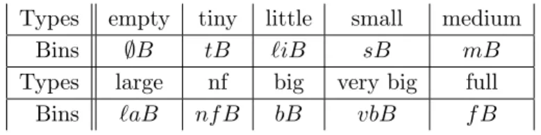
The number of tiny items is denoted bytI, the number of tiny bins is denoted bytB. The abbreviations for cardinalities of the other classes of bins are depicted in Table 1.
Types empty tiny little small medium
Bins ∅B tB ℓiB sB mB
Types large nf big very big full
Bins ℓaB nf B bB vbB f B
Table 1 Abbreviations for bin classes
3
Phase 1 of the Algorithm
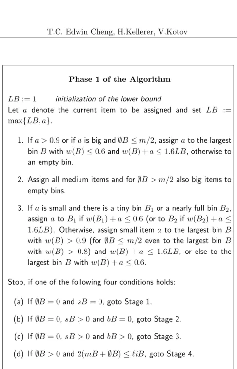
During the algorithm we call LB the current lower bound for the stretching factor of an optimal off-line assignment, starting withLB= 1. In Phase 1 medium items are put alone into bins, big items are put alone into bins as long as more than m/2 bins are empty. When the number of empty bins does not exceed m/2, a big item (like all other large items) is put into the largest small bin in which itfits, i.e. in which the total weight will not exceed 1.6LB, or otherwise into an empty bin. Finally, small items are assigned to small bins if the total weight will not exceed 0.6 or to empty bins. Depending on the four conditions in the end, it will be decided with which stage we continue. A formal description of Phase 1 of the algorithm is depicted in Figure 1.
Some simple properties of the bins after Phase 1 are described in the following lemma:
Lemma 1 During any time of Phase 1 of the algorithm the following properties hold for any bin B:
(a) If w(B) ∈]0.6; 0.8], then B is a medium bin. Moreover, all medium items are alone in bins.
(b) If w(B)>0.8, then B contains a large item. (c) tB+nf B≤1.
(d) sB= 0 or vbB= 0.
Proof: The proofs are straightforward. Assertions (a) and (b) are true by definition of the algorithm. Assertions (c) and (d) follow by induction. We show (c), assertion (d) is straightforward:
Phase 1 of the Algorithm LB:= 1 initialization of the lower bound
Let a denote the current item to be assigned and set LB := max{LB, a}.
1. Ifa >0.9or ifais big and∅B ≤m/2, assignato the largest binB withw(B)≤0.6andw(B) +a≤1.6LB, otherwise to an empty bin.
2. Assign all medium items and for∅B > m/2 also big items to empty bins.
3. If ais small and there is a tiny binB1 or a nearly full binB2,
assign ato B1 ifw(B1) +a≤0.6 (or to B2 ifw(B2) +a≤ 1.6LB). Otherwise, assign small itema to the largest binB
with w(B) > 0.9 (for ∅B ≤ m/2 even to the largest bin B
with w(B) > 0.8) and w(B) +a ≤ 1.6LB, or else to the largest binB with w(B) +a≤0.6.
Stop, if one of the following four conditions holds:
(a) If ∅B = 0 andsB= 0, goto Stage 1.
(b) If∅B = 0,sB >0 andbB = 0, goto Stage 2. (c) If∅B = 0,sB >0 andbB >0, goto Stage 3. (d) If∅B >0 and2(mB+∅B)≤ℓiB, goto Stage 4.
B since the total weight will not exceed 0.6. If a is little, it can be assigned toB or to an empty bin, forming a little bin, or to a large bin or full bin, forming a full bin. Ifais large and is assigned toB, we get either a full bin orB is changed into a nearly full bin. So, in any case tB+nf B ≤1 holds.
Now assume that there is one nearly full bin B, thus no tiny bin. If a fits into B, it is assigned to B and B remains a nearly full bin or becomes full. Ifadoes not fit intoB, we havea >0.5LB, and the bin to whichawill be assigned, will become either a little bin or a full bin.
The next lemma describes the structure of the bins at the end of Phase 1 depending on which Stage is entered in Phase 2.
Lemma 2 The structure of the bins after Phase 1 at the beginning of Stages 1 to 4 can be described as follows:
(a) Stage 1: There are full bins, very big bins, big bins, medium bins plus at most one nearly full bin.
(b) Stage 2: There are full bins, medium bins, little bins and at most one tiny bin or nearly full bin. Moreover we have
2mB≥ℓiB−2. (1)
(c) Stage 3: There are full bins, big bins, medium bins, little bins and at most one tiny or nearly full bin. The bins of B(m/2, m) are all medium bins and thus
mB≥
¹m
2 º
. (2)
(d) Stage 4: There are full bins, medium bins, little bins, at most one tiny bin and empty bins. Moreover we have
Proof: ad (a): The claim follows directly from Lemma 1(a), (b) and (c).
ad (b): The structure of the bins is again a consequence of Lemma 1. Since we do not enter Stage 4, for ∅B > 0 always 2(mB+∅B)> ℓiB holds. Especially for ∅B = 1 we have 2(mB+ 1)> ℓiB. By assigning an item to the last empty bin, the left hand side of the inequality decreases by at most two and the right hand side can increase by at most one. Thus, we get inequality (1).
ad (c): The different types of bins which can exist are a direct conse-quence of Lemma 1. It remains to show that the bins inB(m/2, m) are all medium bins. Remember that big items are put alone into bins as long as∅B > m/2. After the first bin inB(m/2, m) becomes nonempty, big items can be combined with small items and vice versa.
It is easy to show by induction for ∅B ≤m/2 a statement similar to Lemma 1(d) for the big and small items: If ∅B ≤m/2 and bB = 0 or sB= 0, then also bB= 0 or sB= 0 must hold for the rest of Phase 1. It follows, that if bB > 0 and sB > 0 hold at the end of Phase 1, bB >0 and sB >0 must hold already after the last bin in B(1, m/2) becomes nonempty. After this time large items can be assigned to small bins and small items to small bins or bins with load greater than 0.8, none of them to empty bins. Consequently, only medium items can be elements of B(m/2, m).
ad (d): First note that we do not enter Stage 4 (or any other stage) before the number of empty bins is less than or equal to m/2. This means that there is some time when small items are allowed to be packed with big items and vice versa.
ℓiB. Thus, it is only possible that the left hand side of inequality (3) becomes true if there are no bins with a single large item in it and no nearly full bins. The right hand side of inequality (3) follows with an argumentation analogous to (b).
4
Phase 2 of the Algorithm
Phase 2 of the algorithm is split into four stages depending on the structure of the bins after Phase 1. For Stages 1 to 3 we apply a best fit approach. First, we try to put itema into the largest bin in which it fits, and if this is not possible, we assign it to the bin with smallest weight. The formal algorithm for Stages 1 to 3 is depicted in Figure 2.
Phase 2 for Stages 1 to 3 of the Algorithm
Let a denote the current item to be assigned and set LB := max{LB, a}. If ais the (m+ 1)-st item not smaller thanβ, then set LB:= max{LB,2β}.
Assign item a to the largest binB, for which w(B) +a≤1.6LB, else assign ato the bin with smallest weight.
Figure 2 Algorithmic description of Phase 2 for Stages 1 to 3
If our algorithm for (GOBSP) has stretching ratio greater than 1.6, there is a failure item zf which shall be the first item being assigned
to a bin B (w(B) <1) with w(B) +zf >1.6α∗. Then the following
Lemma 3 (a) If zf is assigned to bin B, we have zf ≤ α∗ <
5
3wzf(B)<
5
3. While there are bins with weight not greater than
0.6, the stretching ratio does not exceed 1.6.
(b) Let arriving item a be assigned to bin B with w(B) ≤ 0.9 and
α∗ ≥w(B) + 0.6. Then, w(B) +a≤1.6α∗.
Proof: ad (a): The assertion follows directly from w(B) +α∗ ≥
w(B) +zf >1.6α∗.
ad (b): Asume the assertion does not hold, i.e. ais identical to the failure itemzf. Then we get fromw(B)+zf >1.6α∗ ≥1.6 (w(B)+0.6)
that zf > 0.96 + 0.6w(B). Inserting zf < 53w(B) from Lemma 3(a) into the preceding inequality we getw(B)>0.9, a contradiction.
Before we show that the algorithm works well in Phase 1, we intro-duce some further notation. Consider the bins at the end of Phase 1. Then the very big bins are denoted by V B1, . . . , V Br and the set
{V B1, . . . , V Br} is called the V-group. Analogously, the big bins are
denoted by BB1, . . . , BBs, the medium bins by M B1, . . . , M Bt, and
the small bins by SB1, . . . , SBu, respectively. The corresponding sets
are called B-group, M-group and S-group, respectively. Recall that theM-group consists ofall medium items assigned to separate bins in Phase 1. The nearly full bin N shall be contained in the V-group or B-group, depending on whether w(N) is greater than 0.9 or not. All bin groups shall be sorted in non-increasing order of weight at the end of Phase 1, i.e.
w(V B1)≥. . .≥w(V Br)≥w(BB1)≥. . .≥w(BBs)≥w(M B1)≥. . . . . .≥w(M Bt).
Proposition 1 For Stage 1, the algorithm has stretching ratio 1.6.
Proof: W.l.o.g. assume there is a failure item zf. We distinguish
several cases with respect to the item group to whichzf is assigned:
a) zf is assigned to binM Bt′ (t′ ≤t) of theM-group: Letmt′ denote
the medium item from Phase 1 in M Bt′ and athe first item assigned
toM Bt′ after mt′.
If a 6= zf, then we get wa(M Bt′) +a < 1 and by w(mt′) > 0.6 also
a <0.4. Thus, all bins besidesM Bt′+1, . . . , M Bt have weight at least
1.2. Sincezf is not assigned to M Bt′′ (t′′> t′), we have wzf(M Bt′′)≥
wzf(M Bt′) for t
′′ > t′ and the last item assigned to M B
t′′ before zf
must be greater than 0.6 (otherwise it would be assigned to M Bt′).
Thus, also the bins M Bt′+1, . . . , M Bt have load at least 1.2 and the
total weight of the itemsw(I) would exceed m.
Ifa=zf, due tomt′′< mt′ fort′′ > tan itembmust have been assigned
to M Bt′′ which did not fit into M Bt′, i.e. b+w(M Bt′) >1.6LB. At
that timeLB≥1.2 holds. Therefore,b >1.6·1.2−mt′ ≥1.92−0.8 =
1.12. Thus, at time zf there are m+ 1 items not smaller than mt′
and we conclude α∗ ≥ 2m
t′ > wzf(M Bt′) + 0.6. Lemma 3(b) with
wzf(M Bt′) ≤0.8 contradicts the assumption that zf is assigned to a
bin of theM-group.
b) zf is assigned to binBBs′ (s′≤s) of the B-group: Letbs′ denote
the big item from Phase 1 in BBs′ and a the first item assigned to
BBs′ in Phase 1. Ifa 6= zf, we can argue in a similar way to (a) for
showing that the total weight of the itemsw(I) would exceed m. So assume a =zf. Because of w(BBs′) > w(M Bi) for i= 1, . . . , t at
the end of Phase 1, an item b must have been assigned to each M Bi
which did not fit into BBs′. From LB ≥ 1.2, we get b > 1.6·1.2−
w(BBs′)≥1.92−0.9 = 1.02. Thus , itembis very big andzf is at least
we conclude wzf(BBs′) +zf >1.6·1.6 = 2.56. From Lemma 3(a) we
get zf < 53wzf(BBs′), which gives with the preceding inequality that
wzf(BBs′) > 2.56/(1 + 5/3) = 0.96, a contradiction to the fact that
wzf(BBs′)≤0.9.
c) zf is assigned to bin V Br′ (r′ ≤r) of the V-group: Since at the
end of Phase 1 the weight of each bin of theB-group and theM-group is smaller thanw(V Br′), at timezf to each of these bins an itembhas
been assigned which did not fit intoV Br′. Similar to a) and b) we get
b >1.6·1.2−wzf(V Br′)≥1.92−1 = 0.92, that means at timezf each
bin of the B-group, theM-group and the V-group contains a very big item.
If there are no full bins containing big items at the end of Phase 1, the B-group contains all big items which exist at the end of Phase 1. Therefore, zf is at least the (m+ 1)-st very big item. Hence, α∗ >
0.9 + 0.9 = 1.8, contradicting Lemma 3(a).
If there is a full bin ˜Bwith a big itembat the end of Phase 1, it contains also some small items. Letsdenote the first small item assigned to bin
˜
B. Then at time s all bins with very big items but one are full (and one is at least nearly full). Otherwise s would have been assigned to one of these bins. (Note that very big bins with items greater than 1 would increase LB, so any small item fits into these bins.)
If b is the first item assigned to ˜B, due to the definition of Phase 1, at time s all bins of B(1, m/2) are non-empty. Consequently, all bins except one ofB(1, m/2) with very big items are full.
If s is the first item assigned to ˜B, then no item greater than 0.6 is assigned to ˜Bfor∅B > m/2. Hence, ˜B remains small while∅B > m/2. Because of Lemma 1(a) also in this case all bins but one of B(1, m/2) with very big items are full.
Phase 2. At time zf the total item weight is then greater than
1.1⌈m/2⌉+ 0.9⌊m/2−0.3⌋, an obvious contradiction to w(I) = m.
Let G be a group of bins. If at least one item has been assigned to each bin of Gin Phase 2 (Stages 1 to 3), group Gis called filled. The following lemma is simple but very useful:
Lemma 4 Let G be a filled group of bins each having weight greater thanwat the end of Phase 1. Then all bins but one have weight greater than (0.8 +w/2). Moreover, the average weight of the bins is greater than (0.8 +w/2)if G contains at least two bins.
Proof: It is sufficient to show that there is always at most one binB of group G to which items have been assigned in Phase 2, but which has weight not exceeding (0.8 +w/2). Letabe the new arriving item. Assumeadoes not fit intoB but into a binB′ with smaller weight but no items added. Then,w(B′) +a > w+ 1.6−(0.8−w/2) = 0.8 +w/2. The claim follows.
We show now that the algorithm works well for Stages 2 and 3.
Proposition 2 For Stage 2, the algorithm has stretching ratio 1.6.
a) The M-group is filled before theS-group: Then also theS-group is filled before item zf is assigned. By Lemma 4 all bins but one of
theS-group have weight greater than 0.95 (the last one having weight at least 0.8) and all bins but one of theM-group have weight greater than 1.1 (the last one having also weight at least 0.8). According to inequality (1) we have m ≥t+u ≥ 3
2u−1 and hence u ≤ 2
3(m+ 1). Thus the total weight of the items can be estimated as follows:
w(I) > 1.1(t−1) + 0.95(u−1) + 0.8·2 + 1.1(m−t−u) +zf =
= 1.1m−0.15u−0.45 +zf ≥m−0.55 +zf,
a contradiction tow(I) =m.
b) The S-group is filled before the M-group: Then the first item in Phase 2 assigned to each bin of the S-group is a big item, since items smaller than 0.8 are assigned to a bin of the M-group or to a bin of the S-group to which already a big item has been assigned in Phase 2. Thus, the failure item zf must be assigned to a bin M Bt′
of the M-group. Like in Proposition 1 it is easy to see that zf is the
first item assigned to M Bt′ in Phase 2, otherwise the total weight of
the items would exceedm. Also the first items assigned in Phase 2 to binsM Bt′+1, . . . , M Btare big, otherwise these items would have been
put into M Bt′. Thus, at time zf there are m+ 1 items not smaller
thanmt′ and we concludeα∗≥2mt′ > wzf(M Bt′) + 0.6. Lemma 3(b)
contradicts the assumption thatzf is assigned to a bin of theM-group.
Proposition 3 For Stage 3, the algorithm has stretching ratio 1.6.
a B-group. Again we do a case distinction with respect to the group which is filled first.
a) TheB-group is filled before the other groups: We can continue as in the proof for Proposition 2, noting that inequality (1) is replaced by inequality (2).
b) TheM-group is filled before the other groups: Then the first items assigned in Phase 2 to bins of theM-group are all greater than 0.7 since otherwise they could be assigned to a bin of the B-group. Thus, each bin of theM-group has weight greater than 1.3. By Lemma 3(a) the S-group must be filled before the failure item can arrive and by Lemma 4 all bins but one of the S-group have weight greater than 0.95. Even the smallest bin of the S-group must have weight greater than 0.65. Adding the weights of the items afterzf yields with inequality (1) that
w(I)>⌊m/2⌋1.3 + (⌈m/2⌉ −1) 0.8 + 0.65 +zf > m,
a contradiction tow(I) =m.
c) TheS-group is filled before the other groups: Then the first items assigned in Phase 2 to bins of the S-group are all greater than 0.8 since otherwise they could be assigned to a bin of theM-group. Thus, each bin of theS-group has weight greater than 1.1 (with the possible exception of one bin having weight at least 0.8). Analogously, to part b) of the proof for Proposition 2 we can exclude that the failure item is assigned to a bin of theM-group. Consequently,zf must be assigned
to a bin of the B-group and the M-group must be filled before the B-group. Then, the first items assigned in Phase 2 to bins of the M-group are all greater than 0.7 since otherwise they could be assigned to a bin of the B-group. Again, adding all the item weights gives a contradiction to w(I) =m.
bins each depending on their type after the end of Phase 1. A set of three binsB1,B2,B3forms a3-batch, if is generated from two little bins and one empty bin or one medium. If only small items are assigned to a 3-batch, it is called small 3-batch, if only items greater 0.6 are assigned to a 3-batch, it is calledlarge 3-batch. At the time, when a 3-batch isopened, the “counted” number of little bins, medium bins and empty bins, is reduced appropriately. At the first time when a small item does not fit into a small 3-batch or an item with weight greater than 0.6 does not fit into a large 3-batch, we close the corresponding 3-batch, i.e. no more items are assigned to it. Phase 2 for Stage 4 is depicted in detail in Figure 3.
Lemma 5 Any closed 3-batch has total weight greater than 3.
Proof: a) The assertion is trivially true for small 3-batches, since small items are not greater than 0.6.
Phase 2 for Stage 4 of the Algorithm
Let adenote the current item to be assigned.
1. If a does not fit into the corresponding small 3-batch (large 3-batch), close the batch and open a new small 3-batch (large 3-batch) if possible. If this is not possible, goto 2.
1.1 ais small: Assignato the largest bin of the small 3-batch in which it fits. Goto 1.
1.2 a is medium: Assign a to an empty bin of the large 3-batch, or otherwise to the largest bin in which it fits. Goto 1.
1.3 ais large: If the large 3-batch contains an empty bin and one large item which has been already assigned to this batch, assignato the empty bin. Otherwise, assign it to the largest bin in which it fits. Goto 1.
2. Use best fit, to assign the remaining items into the current open 3-batch and the remaining bins not in batches.
the 3-batch, yielding a total weight greater than 3. If a3 cannot be assigned to B3, it is put into the remaining small bin, yielding total weight greater than (1.6−w(B3)) + 0.8 +w(B3) + 0.6≥3.
Now we are ready to show that the algorithm works well for Stage 4.
Proposition 4 For Stage 4, the algorithm has stretching ratio 1.6.
Proof: Consider the bins to which items are assigned in Step 2 of Stage 4. By Lemma 2(d) there can be two little bins and (at most) one tiny bin which could not be assigned to 3-batches. Moreover, we have three bins (two of them at least little) from the current open 3-batch. Then it can be easily seen that at timezf the total weight of the four
former little bins is greater than 4·0.95 = 3.8 and the total weight of the two other bins exceeds 1.6. By Lemma 5 the bins in batches have average weight 1. Therefore, zf <6−(3.8 + 1.6) = 0.4, contradicting
thatzf is a failure item.
We summarize our results in the following theorem:
Theorem 5 The presented algorithm has stretching ratio 1.6. More-over, the stretching ratio of any deterministic on-line algorithm for (GOBSP) is at least 1.5 for any number m≥6 of machines.
Proof: We get the claimed stretching ratio as combination of Propo-sitions 1, 2, 3 and 4. The lower bound can be obtained from an easy example:
Sendmitems of weight 0.75. If the algorithm puts two of them to the same bin, then sendmitems of weight 0.25. We would getα= 1.5 and α∗ = 1. Thus, the algorithm must distribute the m items of weight
5
Conclusions
In this paper we have presented a relatively simple algorithm with stretching ratio 1.6 for the (GOBSP). Note that the proof of the al-gorithm could be shortened substantially if we apply our alal-gorithm to the on-line bin stretching problem by Azar and Regev. There are still some further interesting open problems: We believe that our algorithm for (GOBSP) can be further improved. Is it possible to adapt our al-gorithm so that we get a stretching factor of at most 1.5 for the on-line bin stretching problem? The two lower bounds for (GOBSP) and for the on-line bin stretching problem are very simple. An improvement of these bounds is not obvious. Specific algorithms for a small number of machines could be developed. Form ≤5, there is still only the lower bound 4.3 for (GOBSP) known.
References
[1] S.Albers,Better bounds for on-line scheduling problems.In: Proc. 29th ACM Symp. on Theory of Computing, pp. 130–139, 1997. [2] Y.Azar, O.Regev, On-line bin-stretching, Theoretical Computer
Science, 268, pp. 17–41, 2001.
[3] E.G.Coffman, J.Csirik, G.Woeginger, Approximate solutions to bin packing problems, In: P.M. Pardalos, M.G.C. Resende (ed.),
Handbook of Applied Optimization, Oxford University Press, 2002. [4] R.L.Graham, Bounds for certain multiprocessor anomalies, Bell
System Technical Journal, 45, pp. 1563–1581, 1966.
[6] H. Kellerer, V. Kotov, M.G. Speranza and Z. Tuza,Semi on–line algorithms for the partition problem,Operations Research Letters, 21, pp. 235–242, 1997.
T.C. Edwin Cheng, Hans Kellerer, Vladimir Kotov, Received Mai 6, 2003
T.C. Edwin Cheng,
Department of Management,
The Hong Kong Polytecnic University, Kowloon, Hong Kong,
E–mail:[email protected]
Hans Kellerer,
Institut f¨ur Statistik und Operations Research, Universit¨at Graz,
Universit¨atsstraße 15, A–8010 Graz, Austria, E–mail:hans.kellerer@uni−graz.at
Vladimir Kotov,
Belarusian State University,
Faculty of Applied Mathematics and Computer Science, Belarusian State University,