A magneto rheological hybrid damper for railway vehicles suspensions

suspensions

Ioan SEBESAN

, Dan BAIASU*

, Gheorghe GHITA

*Corresponding author

_“

POLITEHNICA

”

University of Bucharest, Faculty of Transports,

Splaiul Independentei 313, 060042, Bucharest, Romania

ioan_sebesan@yahoo.com

*

Atelierele CFR Grivita S.A.,

Calea Grivitei 359, 010178, Bucharest, Romania

dan.baiasu@grivita.ro

3

IMS-AR - Institute of Solid Mechanics of the Romanian Academy,

C-tin Mille 15, 010141, Bucharest, Romania

gh_ghita@yahoo.com

Abstract: High speed railway vehicles features a specific lateral oscillation resulting from the coupled lateral displacement and yaw of the wheelset which leads to a sinusoid movement of the wheelset along the track, transferred to the entire vehicle. The amplitude of this oscillation is strongly

dependant on vehicle’s velocity. Over a certain value, namely the critical speed, the instability phenomenon so-called hunting occurs. To raise the vehicle’s critical speed different designs of the suspension all leading to a much stiffer vehicle can be envisaged. Different simulations prove that a

stiffer central suspension will decrease the passenger’s comfort in terms of lateral accelerations of the

carboy. The authors propose a semi-active magneto rheological suspension to improve the vehicle’s comfort at high speeds. The suspension has as executive elements hybrid magneto rheological dampers operating under sequential control strategy type balance logic. Using an original mathematical model for the lateral dynamics of the vehicle the responses of the system with passive and semi-active suspensions are simulated. It is shown that the semi-active suspension can improve the vehicle performances.

Key Words: mathematical model; railway vehicle; hunting oscillations; magnetorheological devices; semi-active suspension.

1. INTRODUCTION

The railway vehicles feature a specific lateral oscillation resulting from the wheelset’s

construction: conical profiled wheels, rigidly mounted on the axle, having opposite conicities. The lateral displacement and yaw coupled oscillations of the vehicle’s wheelset result in a sinusoidal movement of the axle along the tracks. This movement is transferred to

the entire vehicle and it depends on the vehicle’s velocity [1]. For each type of vehicle, if the

speed exceeds a certain value, namely the critical speed, the vehicle’s lateral oscillations become unstable, these oscillations being called hunting. Hunting may induce significant operation problems: running instability, poor ride quality and track wear. From this point of view, an adequate design of the railway vehicle suspensions holds an important role in

maintaining the riding’s comfort and safety parameters. The conventional suspension system

for a passenger vehicle usually has two levels: the axle’s suspension, stiffer, to provide

safety and the suspension of the carbody, softer, to offer best ride quality [2]. Having in view the importance of the lateral oscillations phenomenon numerous authors have dedicated studies to this issue [3–11]. There are possibilities to increase vehicle’s speed by an appropriate design of the passive suspension but this approach proves to have limits. By simulating the vehicle’s response with the lateral dynamics mathematical model its performances for different designs of the passive suspensions are assessed. The identified solutions lead to much stiffer suspensions able to assure the stability of the wheelset movement at higher speeds.

The increase of the critical speed is not the unique criterion of the railway vehicle performances. According to UIC 518 leaflet, the assessment of the vehicle ride quality can be made by measuring the accelerations of the carbody on vertical and lateral directions. The present paper will feature a simulation of the lateral comfort of the vehicle and will use these

performance criteria to improve the vehicle’s suspension concept by introducing semi-active damping devices.

2. THE LIMITS OF THE CLASSICAL SUSPENSIONS

With a view to studying the vehicle’s response in horizontal plan, a mathematical model which simulates the lateral dynamics of a four axle railway vehicle [12, 13] was built up. It is assumed that all the elastic and damping elements forming the classical suspension systems are weightless and have linear characteristics.

Fig. 1 The railway vehicle model for lateral oscillations

z

x

y

x

y

z

x

y

z

2

d

2d

k

k

k

k

y

k

k

k

k

ρ

ρ

ρ

ρ

ρ

ρ

y

y

y

y

y

y

y

Ψ

Ψ

Ψ

Ψ

Ψ

Ψ

v

y

x

k

k

k

k

k

k

k

k

k

k

k

k

k

k

k

k

z

x

y

ψ

φ

Y

Ψ

Φ

Yb1

Ψ

Φ

Y

Ψ

Y

Ψ

Y

Ψ

Y

Ψ

s

O

(ξ

,

,

)

2a

2a

2l

hoo

hob

hcb

hc

c

Under conditions of geometrical, elastic and inertial symmetry, with identical wheel and rail patterns, the equilibrium position of the coach coincides with its median position in relation to the tracks. The rolling surfaces' contact angles are small and the radii of curvature for the rolling treads remain unchanged. Conicity has been considered as having an equal constant value with the rolling surfaces' effective conicity. The mechanical model's geometrical and elastic symmetry facilitates the decoupling of the lateral movements from the vertical ones [1, 5, 10, 11]. To study the vehicle's lateral oscillations, the mechanical model considers the following degrees of freedom: yc, ψc, φc, ybj, ψbj, φbj,yi, ψi, where j=1,2

represents the bogies and i=1 – 4 the wheelsets.

The model highlights the phenomenon of wheel-track contact at large amplitude movement of the axles, characterizing the stability limit cycles, because the flange-rail contact force is considered a linear spring with deadband [3]. The contact forces are

expressed according to Kalker’s linear theory [14]. The resultant creep force cannot exceed the adhesion force. The nonlinear effect of the adhesion limit is treated according to the Vermeulen - Johnson’s nonlinear theory [14] for the case which doesn’t consider the spin creepage. In the model, the tangent track’s irregularities were considered to be periodical, represented with a sinusoid type expression, according to [5, 10]. The isolate variations of the track geometry type bump, was simulated with a single period sinusoid function which considers the irregularity tangent to the track and provides the variation of its dimensions

according to the vehicle’s speed.

The vehicle is considered as being composed of a limited number of rigid bodies, simulating its main parts, connected in between through mechanical weightless linkages: the carbody, the bogies and the wheelsets [15, 16]. Lagrange's equation method was applied in order to establish the movement equations:

k k k

k

Q q

D q

V E q

V E

t  

  

      

 

  

 

) ( ) ( d

d

(1)

where, q is the generalized coordinate, k qkis the generalized speed, E is the kinetic energy, V

is the potential energy, D is the energy dissipation function; Qk is the generalized force

corresponding to the generalized coordinate q . _k

The generalized forces that are considered refer toy and i ψidegrees of freedom of the

wheelsets. The equations of the generalized forces are established using the wheelset efforts diagram presented in [5]. The generalized forces are Q generated by the lateral forces and y_i

i

Q_ due to the yaw moments acting on the wheelsets. Applying Lagrange's equations, the motion equations for the body case, bogies and axles [12, 13] can be obtained. The matrix form of the equations is:

 

M

 

q







 

C

 

q





 

K

   

q



F

(t

)

 

 

 

matrixes of the vehicle’s system,

 

 

 

 

 

 

 

 





 

_{       }

 

 

E 0_{1 1}

 

 

_{ }

 

_{ }

_{ }

F* ₁0

(4)

Table 1. Construction characteristics of the vehicle

Characteristics Symbols Values Units

Body case mass mc 30760 kg

Bogie mass mb 2300 kg

Wheelset mass mo 1410 kg

Carbody moments of inertia Icx

Icz

53596 1661732

kgm2 kgm2

Bogie moments of inertia Ibx

Ibz

2240 2965

kgm2 kgm2

Axles moments of inertia Ioy

Iox

980 100

kgm2 kgm2 Central suspension stiffness

kcx kcy kcz 133 133 473 kN/m kN/m kN/m Axle suspension stiffness

kox koy koz 256 885 904 kN/m kN/m kN/m Central suspension damping

ρcx ρcy ρcz 0 25 18 kN/m/s kN/m/s kN/m/s

Damping of the axle suspension ρoz 3,67 kN/m/s

Wheel tread nominal radius r0 0,460 m

The track’s gauge 2e 1,435 m

The bogie's wheelbase 2a 2,560 m

The distance between bogies 2l 17,2 m

The distance between the secondary suspension springs 2dc 2 m The distance between the primary suspension springs 2do 2 m The distance case center – central suspension hcc 1,24 m The distance axles suspension - bogie center hob 0,01 m The distance central suspension - bogie center hcb 0,06 m

Load on wheel Q 51250 N

The longitudinal creep coefficient f11 9430000 N

The lateral/spin creep coefficient f12 1200 Nm

The spin creep coefficient f22 1000 Nm2

The lateral creep coefficient f33 10250000 N

The effective wheel conicity



The equations (3) are employed both for the study of stability and the system’s response using a numerical integration method of the movement equations, the Runge – Kutta method of 4th order, for which a simulation software has been designed. To simulate the vehicle’s response, the construction characteristics presented in Table 1 are utilized.

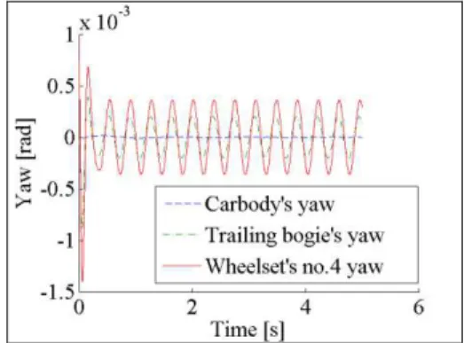
As example, the response of the vehicle with the characteristics in Table 1, launched on a tangent track with periodic irregularities, running with 180 km/h – the maximal testing speed, is presented in figures 2 – 4, indicating that the tracks' perturbations effect is slightly felt at the coach case level, as opposed to the bogie and axles where it persists during the coach's circulation.

The coach's main suspension acts correspondingly and meets the comfort demands inside the coach. The mathematical model of the vehicle previously presented can become a

useful tool to improve the suspension design. A parametric study of the vehicle’s non-linear

stability shows the possibilities of raising the vehicle’s speed through the passive suspension construction.

Fig. 2 The lateral displacement Fig. 3 The yaw oscillations

Fig. 4 The roll oscillations Fig. 5 Axle displacement, v>234.2 km/h

The mathematical model of the vehicle is used to study the vehicle stability. The dynamic system is asymptotically stable if and only if all the eigenvalues of the matrix E have a negative real part [1]. For the vehicle with the characteristics in Table 1, the value of linear critical speed is of 245.6 km/h.

Fig. 6 The bifurcation diagram of the railway vehicle

For the vehicle with the characteristics in Table 1, the stationary solution of the dynamic system is asymptotically stable for speeds less than 245,6 km/h. For speeds greater than 245,6 km/h the solution of the system is unstable. The point of the diagram with the coordinates (245,6; 0) is consequently a bifurcation point – a point where an unstable periodic solution bifurcates subcritically.

Fig. 7 Primary suspension stiffness influence on critical speed

Fig. 8 Primary suspension damping influence on critical speed

Fig. 9 Secondary suspension stiffness influence on critical speed

Fig. 10 The lateral accelerations of the carbody

The solution becomes unstable in the saddle-node bifurcation point with the coordinates (234,2; 9) where the non-linear speed is reached and the amplitude of the wheelset’s movement equals the rail-wheel clearance.

Using the mathematical model, the influence of the suspension damping and of stiffness lateral and longitudinal components on the critical speed of the vehicle is investigated.

The critical speed of the vehicle is strongly influenced by the primary suspension parameters k , ox oy and by the lateral damping of the secondary suspensionk . cy

220

230

240

250

260

120 240 360 480 600 720 840

k

[kN/m]

Vcr lin Vcr nlin

0

100

200

300

400

10 20 30 40 50 60 70 80

₉₀

r

[kNs/m]

Vcr lin Vcr nlin

210

220

230

240

250

1 2 3 4 5 6 7 8 9

k

[MN/m]

Vcr lin Vcr nlin

245.6 234.2 0

1 2 3 4 5 6 7 8 9 10

200 220 240 260 280 300 Vcr [km/h]

In figures 7, 8 and 9 the influences of the mentioned parameters on the vehicle’s critical

speedare presented. The mathematical model previously presented is employed to establish the lateral acceleration of the carbody. The expression of the lateral acceleration, with the notations from Table 1 is:













c y k y h k y k y

m

a       

                 





cb k y

h  

(5)

There are determined the accelerations of the carbody for different values of the central suspension lateral damping coefficient. It can be seen that the result of using more rigid dampers in the central suspension is worse in terms of comfort, due to the coupling effect of those between the lateral oscillations of the bogies and of the carbody – figure 10. This was the reason to consider the use of the semi-active dampers in the secondary suspension of the vehicle.

3. A MAGNETORHEOLOGICAL HYBRID DAMPER

In order to increase the railway vehicle performance, four magneto-rheological controlled dampers will be introduced between the bogies and the carbody to replace the passive dampers. The semi-active systems act to reduce the elastic forces resultant across the vehicle secondary suspension. The semi-active suspension system should continuously control the

vehicle’s response and set the lateral damping coefficient of the secondary suspension to the

appropriate values. Those values are pre-determined in order to meet the safety and comfort demands.

If in the equations (2) the expressions of the lateral damping forces of the secondary suspension are replaced with those given by the magneto-rheological dampers, it will result

the following formulation of the matrix form of the vehicle’s model:

     









    

 









The controllable damping force depends on the relative lateral displacement









applied current intensity.

Using the notations according to figure 1, the relative displacement and speed equations are: bj cb bj c j c cc c

c y h l y h

y         

 _{( 1)} 1

(7) bj cb bj c j c cc c

c y h l y h

y           

 _{( 1)} 1

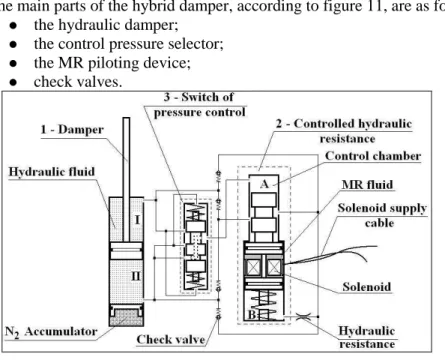
device. In literature this type of damper is known also as MR piloted hydraulic damper. This type of damper features several advantages such as: reduced cost due to the small quantity of fluid required, reduced weight, aspect and overall dimensions similar to those of the passive damper. In fact, the design of the hybrid damper will start from the original passive damper used in the secondary suspension of the vehicle. Figure 11 presents the schematic diagram of a hybrid MR damper proposed by the authors to be included in the vehicle’s semi-active suspension.

The main parts of the hybrid damper, according to figure 11, are as follows:  the hydraulic damper;

 the control pressure selector;  the MR piloting device;  check valves.

Fig. 11 The hybrid MR damper

As control strategy for the MR damper, it is selected a sequential algorithm based on the

balance of forces (balance logic) built to control the system’s vibrations exclusively on an

energy dissipation basis. According to the balance logic, the damping force has to be controlled to balance the elastic force when the carbody is moving away from its equilibrium position – the elastic and damping forces act in opposite directions – and by setting the damping force to a minimal value when the forces have the same direction.

The construction principle of the hybrid MR damper, presented in figure 11 fulfils those requirements. The pressures in the chambers I and II of the damper are controlled by the MR device (the controlled hydraulic resistance) through the pressure switch. The damping force is obtained exclusively hydraulically.

The control system uses speed and movement sensors. When the movement and the speed have opposite signs, the solenoid is supplied with current and the MR fluid is activated. The current intensity is supplied in such way that the cumulated forces in chamber B of the device and of the MR fluid resistance allow the pressure in chamber A to move the piston of the device until the flow between the chambers I and II of the damper would determine the pressure gradient which will produce the damping force according to the control algorithm. The solution proposed for the magneto-rheological device is a double ended piston with a fixed solenoid mounted in a cylinder.

4. THE DESIGN OF THE CONTROL DEVICE WITH MR FLUID

The development of the solution for the MR controlled damper started from the original passive damper type T50/20x210 with the characteristics presented in Table 2. Having in

view that the active surface of the damper’s piston is Ap 16.5cm 2

, the pressure drop is 31

. 30 

pd daN/cm

2 .

Table 2. The characteristics of the passive damper

Characteristic Symbol Value Unit Piston diameter dp 0.05 m Piston rod diameter dt 0.02 m Maximal force F 5000 N

Velocity vp 0.1 m/s

Fluid flow Q 1.65x10-4 m3/s

To establish the dimensions of the controlled hydraulic resistance piston, the surface of the opening,A , required to transfer the flow Q with a pressure drop _o pd will be calculated. The fluid’s flow is considered to be turbulent.

The following equation will be applied:

2 1 2

       

d

o d

p A c

Q (9)

where cd  0.61 characterizes the turbulent flow and 880kg/m 3

is the density of the hydraulic fluid.

The minimal opening surface will be: min  3.26

o

A mm2.

The maximal surface of the opening will be obtained for the free flow between the damper chambers.

The minimal pressure gradient is chosen to be 3 bar – the pressure drop estimated as being generated by the hydraulic resistances on the circuit - and the maximal surface of the opening is max 10.36

o

A mm2.

Considering that the piston of the control device has a diameter of 12 mm, the minimal and maximal forces acting on the piston are:

 _Fmin  34_N – _{the force of the spring in chamber B necessary to close the circuit} between the chambers I and II of by placing the piston of the controllable device in a position that completely closes the hydraulic resistance;

 _Fmax 343_N – _{the minimal force that should be produced by the MR fluid device at} the highest value of the applied current.

The opening is considered to be rectangular with the bigger leg, L , perpendicular on o

the hydraulic resistance piston axle equal to 6 mm.

The strokes of the two extreme positions of the piston are: _cmin  0.54_{mm and} 73

. 1 max 

c mm.

Table 3. The input data of the design

MR fluid type MRF-132LD Maximal velocity of the piston _vmax _0.015m/s Maximal stroke _cmax ₅₁₀3_m Interior diameter of the device _d ₂₂₁₀2_m Diameter of the piston rod  ₈₁₀3

b

d m

Operation temperatures range ₂₀o_C₁₅₀o_C

A wide range of elastomers compatibility -

The constructive model is the one of the double ended device. A design method of a double ended MR damper is presented in [18 - 20]. The input data are presented in Table 3.

To continue the dimensional design, the following parameters are chosen according to the MR fluid characteristics supplied by Lord Corp. [21]. The chosen parameters are shown in Table 4.

Table 4. MR fluid parameters

Shear rate  140s-1 Maximal intensity of the magnetic field H  250kA/m Fluid viscosity   0.25Pa.s Yield stress _c  44.1kPa

Fig. 12 The solenoid of the device

The aim is to maximize the controllability of the device by maximizing the dynamic range coefficient and to minimize the volume of the MR fluid. By imposing those conditions it results the value of the thickness of the gap between the piston and the inner surface of the device [18].

The dimensions of the magnetic circuit composed of the poles, the device case between the poles, the support of the solenoid and the MR fluid [18], considering an applied current of 1.5A, are calculated to design the constructive parameters of the solenoid.

Table 5. The resulting parameters of the MR device

Thickness of the gap 0.4 mm Total force of the device 406.7 N Number of poles 2

Pole width 2 mm

Maximal solenoid diameter 16 mm Solenoid length 30 mm Wire diameter 0.6 mm

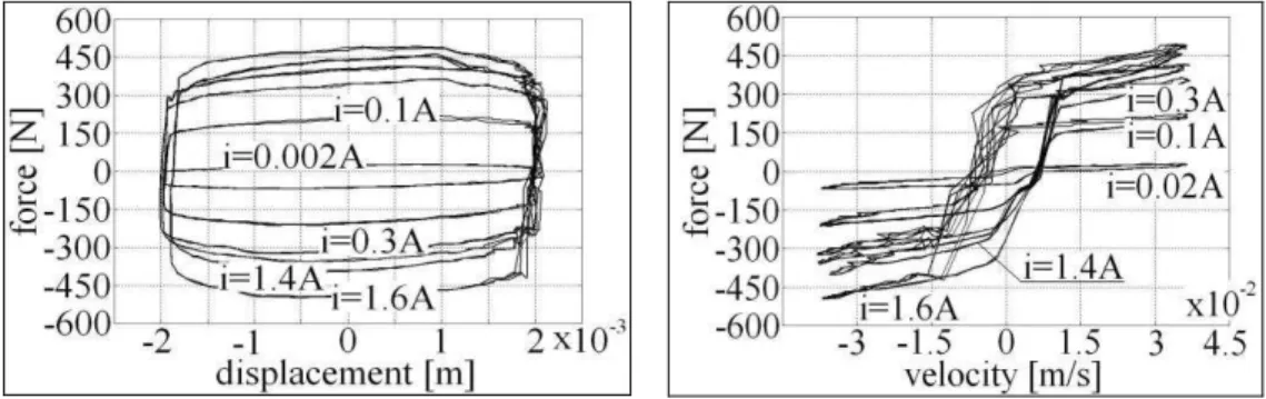
The functional characteristics of the device with magneto-rheological fluid in figures 13 and 14 were experimentally determined.

Fig. 13 Forces vs. displacement diagram Fig. 14 Forces vs. velocity diagram

As it can be seen in the figures above, the maximal value of the force acting on the solenoid piston is greater than the value presented in Table 5. This fact is generated by the number of windings that for technological reasons was greater than the calculated one. The maximal value of the current intensity used in the tests, 1.6A is greater than the estimated 1.5A and this has also an increasing effect on the force. The force of the device is greater than the minimal needed value of 343 N and the device is suitable to control the hydraulic damper.

5. THE OPPORTUNITY OF THE MR SUSPENSION SYSTEMS

In the railway field there are not many vehicles using MR devices. One of the reasons it may be the fact that active technologies are already widely used on high speed trains: the tilting devices which became standard since 1990, the servo-pneumatic and servo-hydraulic active suspensions or the piezoelectric active suspensions. Although extremely effectual, the active suspensions require high powers and sophisticated control technologies. The fact that the

active systems bring supplementary energy to the vehicle may lead to system’s instability.

There are few articles treating the MR suspensions for railway vehicles. In [22] the authors implemented several control strategies used in the automotive industry to a railway vehicle suspension through a computer simulation program which accounts different operational conditions. The results showed that semi-active control improves ride quality of the vehicle. The study, carried on in mid-90th years, evokes the opportunity of using electro-rheological or ferrofluid dampers with the railway vehicle suspension. A study of a MR damper in the secondary suspension of a locomotive is presented in [23]. The paper showed the fact that the semi-active strategy is more efficient than the passive one and the results may be closed to those obtained with an active damper. The design and construction of a MR double ended damper is presented in [20]. The damper model has been established using a testing bench and the ride quality of a vehicle using such a damper, assessed by means of improved simulation software.

The papers [24, 25] are of interest because they present the implementation of an acceleration feed-back control strategy and the positive results of using a MR damper in the

vehicle’s secondary suspension.

A possibility to continue to increase the vehicle’s speed without affecting the comfort is

the use of the controllable suspensions.

In the present paper, the option for controlling the lateral oscillations of the vehicle’s carbody is to use a semi-active control system with a MR fluid device.

The semi-active control systems have the following advantages:

 the oscillations insulation is accomplished by dissipation of energy, similar to the passive devices;

 the system assures full adaptability as active systems do;  no additional energy is introduced in the system;

 the energy needed to operate the semi-active device may be supplied by low power sources;

 there are robust and reliable devices;

 the systems are opened to the unconventional technical solutions.

As operational device of the semi-active suspension, a hybrid MR damper will be introduced in the secondary suspension to control the passive anti-yaw hydraulic damper.

The MR damper brings forward significant benefits in comparison to the classic versions:

 the damping force is controllable in real time;

 it assures great value damping forces at low speeds which is practically impossible with hydraulic dampers;

 the magneto-rheological fluid has its own viscosity which assures a minimal damping force even if the power supply fails;

 the constructive solution is not sophisticated and it is easy to implement for replacing classical dampers.

According to the balance logic control strategy [26], the equation of the semi-active damping force is:





 

_

_

min   

             c c c c c c d c c e c c d y y y y y y F y y F i y y F      (10)

where Fe

 





d y y

dissipation when the hydraulic fluid flows through the control pressure selector’s orifices, reached when the magnetic field isn’t applied (i0).

Having in view the conception of the hybrid damper, in the next pages Fd_minwill be

considered negligible in comparison to the damping forces in semi-active mode. The equation of the damping force will become:





 

  ₍₁₁₎

where is a dimensionless gain factor.

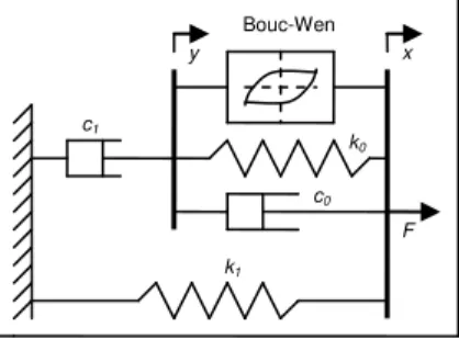
To simulate the result of the semi-active control system utilization with a hybrid MR damper execution element, the modified Bouc-Wen model, proposed by Spencer et al. in 1997 [27] will be used. This model improves the simulated answer of the MR damper in the yield region.

Fig. 15 Modified Bouc-Wen model

The Bouc-Wen models have been conceived aiming from the start to represent the MR dampers. The modified Bouc-Wen model, shown in figure 15, consists in a Bouc-Wen operator which represents the hysteretic behaviour of the damper set in parallel with a viscous damper and a spring simulating the viscous damping and the stiffness of the damper at high velocities, combined with a spring representing the pneumatic accumulator stiffness and a viscous damper to represent the viscous damping effects at high velocities.

The governing equations of the Bouc-Wen model [27] are:

 





F    (12)









c c

y   

    ₀ 1 0 1 _ (13)









z z y x

z      n1     n    (14)

where y is the internal displacement of the damper, A,  ,  are the parameters that determine the shape of the loop, n is the parameter that determines the smoothness of the force-displacement diagram, x₀ is the initial displacement representing the pneumatic accumulator and z

 

To enlighten the influence of the applied current on the MR damper behaviour, it is assumed that the parameters c0, c1,  depend on the voltage applied to the current driver.

There are several formulations of this dependence: linear, third grade polynomial or asymmetric sigmoid function. The linear dependence according to [27] can be expressed with the following equations:

 

   (15)

 

c1  1a  1b (16)

 

c0  0a  0b (17)

where a, c1a and c0a are the values of the parameters at 0 V – passive damper.

The Bouc-Wen model involves 9 parameters that characterize the damper’s behaviour. Those parameters should be determined for each value of the applied current in such way that the predicted response of the damper using the model should be as close as possible to the experimental results obtained through tests. This represents an optimization problem that can be solved through genetic algorithms method. In [26] it is recommended a sequential formulation of the voltage control law similar to the balance logic strategy that would simplify the identification process:

 

 

0 0 , , 0 sgn ,

  

  

x x

x x x x K x

x u

  

  (18)

where  is a dimensionless gain factor experimentally determined to obtain a convenient transmissibility or a minimum r.m.s. acceleration output and K is the measuring calibration factor expressed in _Vmm1_.

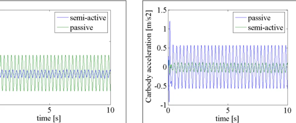
Fig. 16 Carbody acceleration (v=220 km/h,

mm 5 0 

 )

Fig. 17 Carbody acceleration (v=220 km/h,

mm 10 0 

Fig. 18 Carbody acceleration (v=250 km/h,

mm 10 0 

 )

Fig. 19 Carbody acceleration PSD

Several simulations of the employment of the semi-active suspension compared with the use of the classic solution in terms of carbody accelerations are made for different speeds and periodic irregularities amplitudes. To perform those simulations, the controlled damping force generated by the semi-active dampers was included in the mathematical model of the vehicle.

As presented in figures 16 - 19, the use of a semi-active control strategy reduces

significantly the values of the lateral accelerations improving the railway vehicle’s comfort. Figure 19 shows the influence of the semi-active control strategy on the railway vehicle in terms of the p.s.d. value of the carbody acceleration response. There are opened perspectives to study the improvement of passengers comfort using the hybrid MR damper described previously which offers a simple and reliable control of transmissibility of

vehicle’s oscillations from the rolling gear to the carbody.

6. CONCLUSIONS

Having in view that for the passenger trains the safety and comfort conditions are essential, the paper proposes a new type of semi-active suspension controlled by a device with magneto-rheological fluid.

The proposed system may transform any hydraulic damper in a damping system with semi-active control. This application shows the capability of the intelligent fluids to develop a control system more reliable and cost effective than the electro-hydraulic devices.

The design of the piloting device with MR fluid offers possibilities of further developments, being easy adaptable to the specific requirements of the application. For example, if the controlled damper should operate within a wider range of damping forces,

the dimensions of the opening and the piston’s stroke can be modified accordingly. The

control strategy, thought simple, can be very flexible through the dimensionless gain factor which can be adapted according to the specific operational conditions of the vehicle.

REFERENCES

[1] A. H. Wickens, Fundamentals of rail vehicles dynamics, Lisse: Swets& Zeitlinger) 2003.

[2] I. Sebesan, D. Hanganu, The design of the railway vehicles suspensions, Bucharest: Technical Publishing House, 1993.

[3] M. Ahmadian, S. Yang, Effect of system nonlinearities on locomotive bogie hunting stability, Vehicle Syst.

Dyn. 29, 365-84, 1998.

[4] Y. T. Fan, W. F. Wu, Stability analysis of railway vehicles and its verification through field test data, ChIEJ

29, 493-505, 2006.

[5] V. K. Garg, R. V. Dukkippati, Dynamics of Railway Vehicles Systems, Toronto: Academic Press, 1984. [6] Y. He, J. McPhee, Optimization of the lateral stability of rail vehicles, Vehicle Syst. Dyn. 38, 361-90, 2002. [7] S. Y. Lee, Y. C. Cheng, Hunting stability analysis of high-speed railway vehicle trucks on tangent tracks,

J. Sound Vib. 282, 881-98, 2005.

[8] S. Y. Lee, Y. C. Cheng, Nonlinear analysis of hunting stability for high-speed railway vehicle trucks on curved tracks, J. Vib. Acoust. 127, 324-32, 2005.

[9] M. Messouci, Lateral stability of rail vehicles – a comparative study, J. Eng. Appl. Sci. 4, 13-27, 2009. [10] I. Sebesan, Railway Vehicles Dynamics, Bucharest: Technical Publishing House, 1995.

[11] I. Sebesan, I. Copaci, Theory of elastic systems for railway vehicles, Bucharest: Matrix Publishing House, Rom. Editions, 2008.

[12] I. Sebesan, D. Baiasu, Gh. Ghita, Study of the railway vehicle suspension using the multibody method,

INCAS Bull. 3, 89-104, 2011.

[13] I. Sebesan, D. Baiasu, Matematical model for the study of the lateral oscillations of the railway vehicle,

U.P.B. Sci. Bull. 74, 51-66, 2012.

[14] J. J. Kalker, Wheel-rail rolling contact theory, Wear 144, 243-61, 1991.

[15] A. A. Shabana, Dynamics of Multibody Systems, Cambridge: Cambridge University Press, 2005. [16] A. A. Shabana, Computational dynamics, Hoboken: John Wiley & Sons Ltd, 2010.

[17] O. Polach, On non-linear methods of bogie stability assessment using computer simulations, J. Rail Rapid

Transit 220, 13-27, 2006.

[18] T. Sireteanu, Gh. Ghita, D. Stancioiu, Magneto-rheological fluids and dampers, Bucharest: BREN Publishing House, Rom. Editions, 2005.

[19] G. Yang, B. F. Spencer Jr., J. D. Carlson, M. K. Sain, Large-scale MR fluid dampers: modeling and dynamic performance considerations, Eng. Struct. 24, 309-23, 2002.

[20] Y. K. Lau, W. H. Liao, Design and analysis of magneto-rheological dampers for train suspension, J. Rail

Rapid Transit 219, 261-75, 2005.

[21] ***Lord Corporation, Magneto-rheological Fluid MRF-132LD, Product Bulletin, 1999.

[22] H. R. O’Neal, G. D. Wale, Semi-active suspension improves rail vehicle ride, Comput. Control Eng. J. 5, 183-8, 1994.

[23] Y. Shen, S. Yang, C. Pan, H. Xing, Semi-active control of hunting motion of locomotive based on magnetorheological damper, Int. J. Innov. Comput. I. 2, 323-29, 2006.

[24] D. H. Wang, W. H. Liao, Semi-active suspension systems for railway vehicles using magnetorheological dampers. Part I: system integration and modeling, Vehicle Syst. Dyn. 0, 1-21, 2009.

[25] D. H. Wang, W. H. Liao, Semi-active suspension systems for railway vehicles using magnetorheological dampers. Part II: simulation and analysis, Vehicle Syst. Dyn. 0, 1-33, 2009.

[26] T. Sireteanu, Gh. Ghita, D. Stancioiu, C. W. Stammers, Semi-active vibration control using balance-logic strategy: modeling and testing, RJAV I, 31-8, 2004.