Inferring internal properties of Earth's core dynamics and their evolution from surface observations and a numerical geodynamo model

www.nonlin-processes-geophys.net/18/657/2011/ doi:10.5194/npg-18-657-2011

© Author(s) 2011. CC Attribution 3.0 License.

Nonlinear Processes

in Geophysics

Inferring internal properties of Earth’s core dynamics and their

evolution from surface observations and a numerical

geodynamo model

J. Aubert and A. Fournier

Institut de Physique du Globe de Paris, UMR7154, INSU, CNRS – Universit´e Paris-Diderot, PRES Sorbonne Paris Cit´e, 1 rue Jussieu, 75238 Paris cedex 5, France

Received: 28 June 2011 – Revised: 23 September 2011 – Accepted: 3 October 2011 – Published: 12 October 2011

Abstract. Over the past decades, direct three-dimensional numerical modelling has been successfully used to reproduce the main features of the geodynamo. Here we report on ef-forts to solve the associated inverse problem, aiming at in-ferring the underlying properties of the system from the sole knowledge of surface observations and the first principle dy-namical equations describing the convective dynamo. To this end we rely on twin experiments. A reference model time se-quence is first produced and used to generate synthetic data, restricted here to the large-scale component of the magnetic field and its rate of change at the outer boundary. Starting from a different initial condition, a second sequence is next run and attempts are made to recover the internal magnetic, velocity and buoyancy anomaly fields from the sparse surfi-cial data. In order to reduce the vast underdetermination of this problem, we use stochastic inversion, a linear estimation method determining the most likely internal state compatible with the observations and some prior knowledge, and we also implement a sequential evolution algorithm in order to invert time-dependent surface observations. The prior is the multi-variate statistics of the numerical model, which are directly computed from a large number of snapshots stored during a preliminary direct run. The statistics display strong correla-tion between different harmonic degrees of the surface obser-vations and internal fields, provided they share the same har-monic order, a natural consequence of the linear coupling of the governing dynamical equations and of the leading influ-ence of the Coriolis force. Synthetic experiments performed with a weakly nonlinear model yield an excellent quantita-tive retrieval of the internal structure. In contrast, the use of a strongly nonlinear (and more realistic) model results in less accurate static estimations, which in turn fail to constrain the unobserved small scales in the time integration of the

Correspondence to: J. Aubert (aubert@ipgp.fr)

evolution scheme. Evaluating the quality of forecasts of the system evolution against the reference solution, we show that our scheme can improve predictions based on linear extrapo-lations on forecast horizons shorter than the systeme-folding time. Still, in the perspective of forthcoming data assimila-tion activities, our study underlines the need of advanced es-timation techniques able to cope with the moderate to strong nonlinearities present in the geodynamo.

1 Introduction

the measurement errors, which have become very small at the age of satellite magnetic observation. As an illustration of a non-uniqueness problem, closure constraints are needed in order to perform core flow inversions (most recently the quasi-geostrophic assumption, Pais and Jault, 2008). The nonlinearity involved in the core flow problem is an instance of a spatial resolution problem, in the sense that the unre-solved small scales of the magnetic field are responsible for part of the observed secular variation at large scale, in a way which is difficult to predict. This, in turn, complicates the evaluation of the flow large scales (Eymin and Hulot, 2005; Gillet et al., 2009). One elegant, yet not much explored way to handle both problems is through enforcing dynamical con-sistency of the solutions, that is, solving for a velocity field with a time evolution consistent with first principle evolu-tion equaevolu-tions. The problem of determining core flow then becomes an inverse problem where an initial condition is sought, the evolution of which will subsequently explain and predict the observations at various points in time, hereby all dynamically connected together. Along these lines, the now expanding field of geomagnetic data assimilation aims at op-timally combining physical laws and observations of Earth’s core dynamics (see Fournier et al., 2010, for a recent review). This expansion capitalizes on the progress made over the last twenty years by data assimilation techniques in other fields of research, most importantly (from the viewpoint of core dynamics), atmospheric dynamics and physical oceanogra-phy. Regarding the specific three-dimensional Kalman filter which is central to the following, the interested reader is re-ferred to the authoritative monograph by Evensen (2009) for a detailed description of its theoretical foundations, and its extension to nonlinear problems in the form of the so-called ensemble Kalman filter. For further reading, Kalnay (2010), Brasseur (2006), Elbern et al. (2010) and Houser et al. (2010) review recent applications of the Kalman filter to the analy-sis of the atmosphere, of the ocean, of air quality and of land surfaces, respectively.

First principle equations suitable for the direct modelling of core dynamics (Braginsky and Roberts, 1995) are now routinely solved numerically, and have had considerable suc-cess in reproducing the first-order features of the geomag-netic field: morphology and dipole dominance of the field, secular variation and reversals (main advances recently re-viewed by Christensen, 2011). These equations include the induction equation, Navier-Stokes equation with convection described in the Boussinesq approximation, and an equation for the transport of a buoyancy field (which, in the Earth’s core, is of both thermal and chemical origin). The main difficulty faced by these three-dimensional, self-consistent simulations is the current impossibility to reach numerically the physical parameters of natural dynamos. This is related to the great disparity between the diffusion coefficients of the thermal, chemical, magnetic and velocity fields. As the situation is not likely to improve in the foreseeable future, progress in the field has been achieved over the recent years

by identifying and scaling phenomena where some or all of these diffusivities play only a secondary role. For instance, a large set of numerical models has revealed that the magnetic field strength does not depend on any diffusion coefficient, only on the available power to drive the dynamo (Christensen and Aubert, 2006; Aubert et al., 2009). A connected study (Christensen et al., 2010) showed that a morphological simi-larity can be obtained between the geomagnetic field and the output of numerical dynamos if only three time scales are in reasonable proportion when compared to their Earth counter-parts: the rotation period of the planet, the characteristic time scale of advection of the magnetic field by the fluid flow, and the characteristic time for the diffusion of the magnetic field. Here we wish to use the information and dynamically con-sistent solutions provided by numerical geodynamo models in order to carry out inverse modelling. Our long-term aims are (i) to estimate the dynamical state of Earth’s core from surface observations, (ii) to assess the extent to which such estimations are affected by (or immune to) non-uniqueness and spatial resolution problems, and (iii) to determine the magnitude of the associated errors. Linear estimation of the system state invisible parts (also called Kalman filtering or stochastic inversion) is a method of choice for this type of problem. Its efficiency is classically tested through the pro-cedure of synthetic (twin) experiments: a reference solution is first computed, and used to generate a catalog of surface data, which are in turn used to recover the solution, start-ing from a wrong initial guess. Previous attempts (Liu et al., 2007) used parameterised, ad-hoc covariance properties to perform such estimations, and focused mostly on the evolu-tion of the observed, surficial part of the system. The nov-elty of our approach stands in a preliminary numerical com-putation of the system multivariate covariance properties. This approach has already been used in a companion paper (Fournier et al., 2011), addressing the two-dimensional core flow problem described above. Here we proceed to the deter-mination of the three-dimensional internal structure, which can then be used as an initial condition for time evolution, opening the way to data assimilation practice. In the fol-lowing, Sect. 2 presents the numerical model and inversion technique. Section 3 presents the results of the numerical experiments, which are then discussed in Sect. 4.

2 Model and methods

2.1 Numerical geodynamo model

Our numerical model is formulated as in Aubert et al. (2009). We solve for the velocity field u, magnetic field B, and co-density (or co-density anomaly) fieldCin a spherical fluid shell between radiiri andro, of aspect ratiori/ro=0.35 rotating

∂u

∂t = −u· ∇u−2 ez×u− ∇P +RaQ

r

roC+(∇ ×B)×B+E∇

2_{u, (1)}

∂B

∂t = ∇ ×(u×B)+Eλ∇

2_{B, (2)}

∂C

∂t = −u· ∇C+Eκ∇ 2_C+S

T /ξ, (3)

∇ ·u=0, (4)

∇ ·B=0. (5)

Here r is the radius vector. The fundamental scales under-lying the dimensionless scheme are the inverse shell rotation rate−1 _{for time, the shell gapD for length,(ρµ)}1/2_D for magnetic induction, whereρ is the fluid density and µ

the magnetic permeability of the fluid. The kinematic, mag-netic and thermal Ekman numbers are defined as

E= ν

D2, (6)

Eλ= λ

D2, (7)

Eκ = κ

D2. (8)

Hereν,λ,κare respectively the viscous, magnetic, and ther-mochemical diffusivities of the fluid. As detailed in Aubert et al. (2009), the distribution of boundary mass anomaly fluxes can be determined from a parameterised thermody-namical model of Earth’s core evolution. Here we choose an idealised situation which is thought to be representative of Earth at present (Lister, 2003), where the mass anomaly fluxF originates entirely from the inner boundary, and the outer boundary has null mass anomaly flux. The Rayleigh numberRaQis thus

RaQ= goF

4πρ3_D4, (9)

wheregois gravity at radiusr=ro. As shown in Aubert et al. (2009) the dimensionless volume sink term for mass anomaly corresponding to this situation isST /ξ= −3/(r_o3−r_i3). The other boundary conditions at both boundaries are no-slip for velocity, and insulating for the magnetic field. The numerical implementation PARODY-JA is used in this study (Dormy et al., 1998; Aubert et al., 2008). The fields u, B are expanded into toroidal and poloidal scalars, which, together with the scalarC, are described using a finite-difference scheme in the radial direction with up to 160 grid points, and a spherical harmonic decomposition in the lateral directions up to degree and order 133.

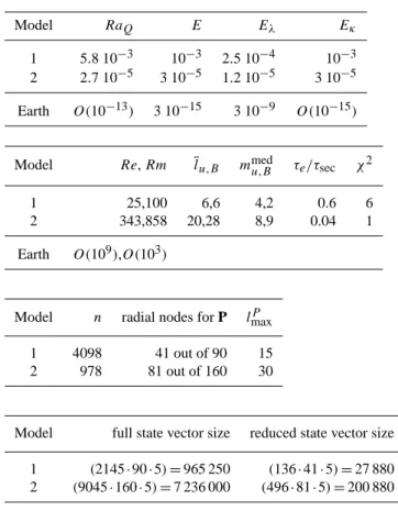
Table 1 summarizes the properties of the two models which have been integrated for this study. The models have been chosen so as to provide end-members in physical com-plexity and semblance to the geomagnetic field. Model

Table 1. Properties of the numerical models used for the study. First

row: input parameters (see main text for definitions). Second row: output parameters. Earth’s core values are estimated in Christensen

and Aubert (2006). The mean harmonic degreeslu,Bin the velocity

and magnetic field are as defined in Christensen and Aubert (2006). The median harmonic ordersmmed_u,B are the orders which, on aver-age, separate the velocity and magnetic power spectra in two do-mains of equal energy. Thee-folding timeτeand secular variation

timeτsecare as defined in Lhuillier et al. (2011a,b). The

morpho-logical semblance to the geomagnetic fieldχ2is defined according to Christensen et al. (2010). Bottom two rows: parameters rele-vant to the determination of the model covariance matrix P. Unless otherwise noted, the numerical experiments use a covariance

ma-trix which is determined from the numbern of free run samples

reported in the table. Also reported are the number of radial nodes used for the determination of the matrix, the degree and orderl_maxP up to which this matrix is determined, the size of the state vector (complex coefficients) and the number of coefficients involved in the determination of P (or reduced state vector size).

Model RaQ E Eλ Eκ

1 5.8 10−3 10−3 2.5 10−4 10−3

2 2.7 10−5 3 10−5 1.2 10−5 3 10−5

Earth O(10−13) 3 10−15 3 10−9 O(10−15)

Model Re,Rm lu,B mmed_u,B τe/τsec χ2

1 25,100 6,6 4,2 0.6 6

2 343,858 20,28 8,9 0.04 1

Earth O(109),O(103)

Model n radial nodes for P l_maxP

1 4098 41 out of 90 15

2 978 81 out of 160 30

Model full state vector size reduced state vector size

1 (2145·90·5)=965 250 (136·41·5)=27 880

2 (9045·160·5)=7 236 000 (496·81·5)=200 880

Model 1

Model 2

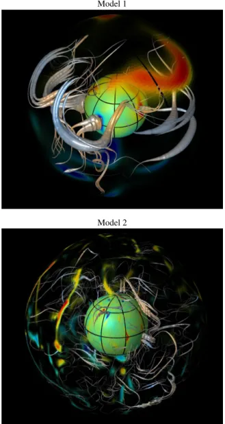
Fig. 1. Dynamical magnetic fieldline imaging (DMFI)

representa-tion of the numerical models magnetic field line structure. The mag-netic field lines are rendered as grey tubes, with thicknesses propor-tional to the local magnetic energy density. The inner core surface is color-coded according to the radial magnetic field strength. The outer surface is color coded similarly, and made transparent with an opacity proportional to the radial magnetic field strength (see Aubert et al., 2008, for further details).

Christensen et al. (2010). The main morphological differ-ence arises from the high concentration of magnetic flux into a small number of patches, and also in the lack of equatorial field features (which was not taken into account in the rat-ings of Christensen et al., 2010). Model 2 fares much better with respect to semblance to the geomagnetic field. It can also be considered a physically more suitable model because the three time scales mentioned in the introduction (magnetic advection, magnetic diffusion, rotation period) are in better

proportion when compared to the Earth than for model 1. The ratio of the magnetic diffusion and magnetic advection time scale is the magnetic Reynolds number Rm, which is very close to the value of about 800 which can be expected in the Earth’s core if surface velocity estimations are rep-resentative of the deep flow (Christensen and Tilgner, 2004). The ratio of the length of day and the magnetic diffusion time scale is the magnetic Ekman numberEλ, which in model 2

is one order of magnitude closer to the valueEλ≈10−9

ex-pected in the core (e.g. Christensen and Aubert, 2006). As a consequence of the higher Reynolds numbers, model 2 also has stronger nonlinearities than model 1, and the effect of a stronger magnetic advection results in an apparent decorrela-tion between the surface and internal magnetic structures (see Aubert et al., 2008, and also Fig. 1). The increased temporal complexity of model 2 can be quantified using the ratio of the

e-folding time of the systemτe, or time constant for the

expo-nential divergence of two infinitesimally close solutions (Hu-lot et al., 2010b; Lhuillier et al., 2011a), to the characteristic time scale for secular variationτsec(Christensen and Tilgner, 2004; Lhuillier et al., 2011b). The increased spatial complex-ity can be evaluated through the mean harmonic degreeslu,B,

as defined in Christensen and Aubert (2006), and median har-monic ordersmmed_u,Bin the power spectrum of the velocity and magnetic field. It is important to mention that although they are quite different, both models have more than half of their energy within the harmonic order rangem=0−13, which means that there is reasonable hope that surface observations supplied within the same spectral range could constrain well the internal structure.

2.2 Rescaling the model output

Although this is not fundamental when only synthetic data are used, any attempt to integrate time-dependent geomag-netic data into a numerical model will require the dimension-less model output to be rescaled to the geophysical world. If the model operated at the same parameter values as the Earth’s core, it would be enough to use the canonical scales presented in the last section. However, as the model operates far from Earth’s core conditions, we have to resort to units underlain by scaling principles known (or thought) to hold both in the model and in the Earth’s core, so that the various quantities, once presented in these new units, should have similar values in the model and in the core.

Following previous work on the secular variation time scale (Christensen and Tilgner, 2004; Lhuillier et al., 2011b; Fournier et al., 2011), time will be presented in units of

scenario presented in Aubert et al. (2009), one magnetic field unit then amounts to 1.7 mT for the present Earth. Fi-nally, the relationship between the convective power, co-density and velocity (Eq. A1 in Christensen and Aubert, 2006) prompts to present the co-density field in units of

pτsec/goD. Using again the high-power scenario, one

co-density unit amounts to 10−5kg m−3.

2.3 Best linear unbiased estimate of the internal structure from surface data

For a given discrete instanttiin a numerical dynamo

simula-tion, we define a (column) state vector (superscriptTdenotes the transpose)

x(ti)=[up_lm(rj,ti),ut_lm(rj,ti),B_lmp(rj,ti), B_lmt (rj,ti),Clm(rj,ti)]T,

(10)

which contains the complex values of the poloidal (super-script p), toroidal (superscript t) harmonic scalars of the fields u,B and the co-densityC, for each harmonic degree and orderl,m on the nodes j of the radial grid. The full size of x is on the order of one to ten million elements (see Table 1). Covariance matrix calculations presented in this study however use a version of x which is decimated by tak-ing a subset of radial nodes and harmonic coefficients (see Sect. 3.1 and Table 1), yielding a typical size on the order of ten to a hundred thousand elements. The state vector is cen-tered and normalised for the time series to have zero mean and unit variance.

We assume that the various elements in x have a Gaussian distribution, with probability density function (pdf)P(x)∝

exp(−x′P−1x/2), where P is called the covariance matrix of the model and the prime symbol denotes the transpose com-plex conjugate. The validity of the Gaussian assumption is explored in Fournier et al. (2011). Some deviations from a Gaussian behavior can be expected, in which case the best linear estimate about to be derived is not optimal anymore in the sense of maximum a-posteriori pdf, but still remains the estimate of minimum variance.

The state vector has an observable part and a hidden part. Our goal is to provide an estimate of the hidden part from the observable part. We define an observation operator H which extracts its observable part from x. The observation opera-tor is thus a rectangular matrix with a number of rows equal to the size of the observations y and a number of columns equal to the size of the state vector x. Because we are dealing with the equivalent of global field models at the core-mantle boundary, and given their current resolution limits (e.g. Olsen et al., 2010), we define the observable part of the state vector as the poloidal magnetic fieldB_lmp(ro)at the outer boundary

up to degree and order 13. The corresponding observation operator contains ones in the entries corresponding to an ob-served quantity and zeros otherwise. The operator contains an additional sub-block when the rate of change ofB_lmp (ro)

is observed as well (up to degree 13). Considering the ra-dial part of the induction Eq. (2) on the fluid side of the outer boundary, where the velocity field vanishes, we obtain

∂B_lmp

∂t (ro)=Eλ∇ 2_Bp

lm(ro). (11)

Prescribing the time derivative of the outer boundary poloidal magnetic field is thus equivalent to prescribing the ra-dial component of ∇2B_lmp. The sub-block dedicated to

∂B_lmp(ro,ti)/∂t thus contains a discrete Laplacian operator

written on the fluid side of the outer boundary. The vector Hx comprises up to 210 elements.

Our inverse problem seeks a state vector x such that

Hx+ǫo=y, (12)

where y is a set of observations, statistically centered and normalised using the same means and variances as those used for x. In a general context, the observations bear some error

ǫo, with a covariance matrix R=E(ǫoǫo′), whereEstands

for the expected value. In other words, the likelihood of y if x is realised isP(y|x)∝exp(−(y−Hx)′R−1(y−Hx)/2). Given the above mentioned sizes of x and y, the problem posed by Eq. (12) is vastly underdetermined. Our preferred estimate of x is the best linear unbiased estimate, which min-imizes the functional

J(x)=(y−Hx)′R−1(y−Hx)+x′P−1x. (13) This estimate is the most likely given the data and model co-variance properties (see Fournier et al., 2011, for details). Looking for the extrema ofJ(x)one finds the best linear in-verse solution, which takes a simple form when x is centered:

x=Ky, (14)

with the Kalman gain matrix

K=PH′ _HPH′_+R−1_{. (15)}

Equation (15) is ubiquitous in geomagnetic field modelling (Gubbins, 1983) and core flow modelling (review in Fin-lay et al., 2010a). In both cases it is usually referred to as stochastic inversion, but we also note that it is formally iden-tical to one of the Kalman filter equations (e.g. Fournier et al., 2010). The stochastic inversion will be more efficient when P contains strong correlations between the observed and un-observed parts of the state vector. Our primary goal being to test the accuracy and prediction power of the inversion with synthetic data, we consider the data error-free i.e.ǫo=0 and

In a time-dependent context, the stochastic inverse can be used to initialise the numerical model and perform forecasts of the system evolution. This forms the backbone of se-quential data assimilation. At a given later time where the numerical model has updated the state vector to a value xf (the forecast), an analysis of the system can be performed by comparing the observed part of the forecast Hxf to the ob-servations y available at the analysis time. The state vector is then corrected to the new value xasuch that

xa=xf+Ky−Hxf, (16)

The analysed state vector is then used as a new starting condi-tion, completing an assimilation cycle. Each time the system is corrected, P should be updated according to a correspond-ing evolution equation (the set of equations updatcorrespond-ing P and the state vector and describing their time evolution is called the Kalman filter, Kalman, 1960). As this is a computation-ally very intensive task, P is often assumed to be time inde-pendent, which amounts to assuming that although the anal-ysis tends to reduce the error on the system state knowledge, the nonlinear dynamics operating between two analyses re-stores this error back to its natural (free run) value. When using such a frozen covariance matrix, the assimilation tech-nique is referred to as optimal interpolation (or OI, see e.g. Kalnay, 2003, for a review).

Atmospheric and oceanic data assimilation usually resort to matrices operating in physical space (Kalnay, 2003, §5.4). There, the choice of an a-priori defined correlation length re-sults in sparse banded structures which are easy to process, even with state vectors with sizes comparable to what is re-ported in Table 1. The accuracy of such an approach depends on whether in-situ measurements are available with sufficient quantity. The geomagnetic assimilation case is completely different because of the lack of in-situ measurements. In that context, the information cannot be efficiently and accurately propagated radially downward past the correlation length if the above approach is employed. We thus need to process a covariance matrix with a full structure, obtained in spectral space, in order to perform an accurate and efficient propa-gation of this information. It can then be understood that practical computational considerations set a limit on the size of such a matrix, which can thus update only a subset of the state vector. This limitation was not present in our previ-ous study (Fournier et al., 2011), where the two-dimensional character of the problem permitted high-resolution inver-sions. When used with this limitation, scheme (16) can be unstable due to the deleterious influence of the uncorrected variables. Here we control these instabilities using a slightly modified version of the OI scheme, where only a fractionβ (0≤β≤1)of the forecast is re-injected at analysis stage xa=βxf+Ky−βHxf, (17) Ifβ=0 then at each analysis time, the system is set to x=0 (time average of the dynamo simulation) before the analysis

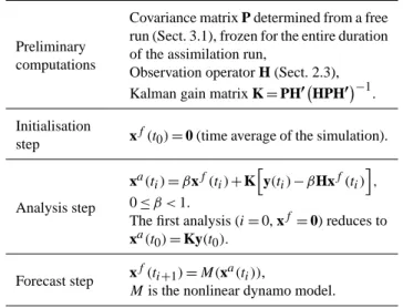
Table 2. Summary of the time-dependent assimilation scheme used

in this study (noise-free data).

Preliminary computations

Covariance matrix P determined from a free run (Sect. 3.1), frozen for the entire duration of the assimilation run,

Observation operator H (Sect. 2.3),

Kalman gain matrix K=PH′ _HPH′−1_.

Initialisation

step x

f_(t

0)=0 (time average of the simulation).

Analysis step

xa(t_i)=βxf(t_i)+Khy(t_i)−βHxf(t_i)i, 0≤β <1.

The first analysis (i=0, xf=0) reduces to xa(t0)=Ky(t0).

Forecast step x

f_(t

i+1)=M(xa(ti)),

Mis the nonlinear dynamo model.

is performed; each analysis is thus an inverse of the cor-responding data with no memory from previously inversed data. Ifβ=1 the analysis corrects the full forecast resulting from the previous time integration; the whole forecast is thus re-injected for the next analysis cycle. A value ofβ between 0 and 1 will help mitigate the two possibilities. There is no theoretical justification for the introduction ofβin the analy-sis. The justification is practical, as we observed that the use of the regular Kalman filter analysis (β=1) resulted in over-energetic estimates of those variables not directly impacted by the observations and the truncated covariance matrix P.

3 Results

3.1 Computation and structure of the model covariance matrix

A correct determination of P is central to the quality of the inversion (14)–(15). Here we approximate P using the mul-tivariate statistics of the numerical model. This matrix is thus computed during a preliminary “free run” of the model, where a numerical integration is performed and a large num-ber n (see Table 1) of state vector snapshots x(ti)are ex-tracted, with a typical time lag between the snapshots on the order of thee-folding time of the system to ensure decorre-lation between snapshots. In terms of classical dynamo time scales, the duration of the free run is 17.5 magnetic diffu-sion timesD2/λ. In terms of the advective time rescaling used in this study, the duration is about 580τsec, amounting to 290 000 yr ifτsec=500 yr. Once each time series of the state vector components is centered and normalised to unit variance, if the vectors x(ti)are stored as columns into a

outer boundary poloidal magnetic field coef

ficients

poloidal velocity field coef

ficients inside the shell

radius

0

0.1

0.2

0.3

0.

0.5

0.6

0.7

0.8

0.9

1

track 1

track 2

modulus of correlation coef

ficient

m=0 _m=1

m=2 _m=3

m=4 _m=5

m=6

m=7 m=8 _m=9

track 1 track 2

corr. coeff. modulus 0 0.2 0.4 0.6 0.8 1

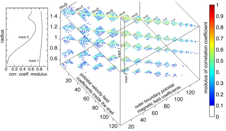
Fig. 2. Representation of the coefficients of the covariance matrix P involved in the determination of the stochastic inverse matrix K. At

five different radial levels (vertical axis), the colored squares map the modulus of the correlation coefficients between the surface poloidal magnetic field harmonic coefficients (first horizontal axis) and the poloidal velocity field coefficients (second horizontal axis). Harmonic coefficients are ordered according to a one-dimensional scheme where all admissible values oflare grouped together for each given value of m. These correlation coefficients are computed from a free model run (here from model 1) wheren=4098 instantaneous state vectors spaced by 0.3τsec(half ane-folding time) each are extracted. The coefficients are computed up to degree and orderlmaxP =15, which corresponds to

the one-dimensional parameterlm=120. Two vertical tracks are drawn, representing the evolution of the correlation coefficients with depth form=4, between harmonicslobs=5 of the observed field andldeep=4 of the deep field (track 1), and between harmonicslobs=5 and

l_deep=12 (track 2).

P= 1 n−1XX

′_{. (18)}

For reasons of storage and cpu time limitations, about half of the numerical grid radial nodes are used to determine P, the remaining nodes (see Table 1) being computed by linear interpolation. We have checked that this has no impact on the quality of the inversion. Likewise, only harmonic coef-ficients up to degree and order l_maxP are retained. In order to capture the correlations involving the dominant scales of the system, we setl_maxP so that it exceeds bothmmed_u,B andlu,B

(see Table 1). The convergence of the coefficients defining P is checked by monitoring the effect of doubling and decimat-ing the number of samples used to build the matrix (see also Fig. 8a).

According to Eq. (15), not all coefficients of P are actu-ally needed to compute the matrix K: only the correlations involving one observed quantity have an effect on the result. We thus represent on Fig. 2 sub-blocks of P displaying the

correlations betweenB_lmp (ro)and one of the fields (hereup_lm

at various radii; the structure is similar for other fields, with some differences detailed below). Harmonic coefficientslm

have been ordered along a one-dimensional lexicographic scheme gathering all possible degrees (up tolP_max=15 in this case) for each given order.

In the case of model 1, Fig. 2 shows that the internal structure is linearly coupled with the surface observations, as could be expected from the visualisation presented in Fig. 1. Correlation coefficients are indeed up to 0.9 when correla-tions betweenB_lmp(ro)(or its time derivative) with another

nonlinear couplings. The dominant azimuthal wavenumber of the surface magnetic field thus reflects that of the internal convection flow, as expected from a dynamo mechanism (e.g Olson et al., 1999; Aubert et al., 2008) where the magnetic energy is sustained through stretching, twisting and folding of the magnetic field lines by a columnar convection flow. The correlations tend to peak at or around the dominant az-imuthal wavenumber of the dynamo, as measured bymmed_u,B

in Table 1. The influence of the leading equatorial sym-metry properties of the flow and magnetic field is seen in the checkerboard pattern of the correlations: iflobsandldeep are respectively the harmonic degree ofB_lmp(ro)(or its time derivative) and the internal field, thenlobs+ldeep needs to have odd parity if the internal field isup_lm,ClmorB_lmt , and even parity if the internal field isB_lmp andut_lm. As the ra-dius decreases towards the inner-core boundary, the correla-tion matrix displayed in Fig. 2 exhibits an upper triangular structure: coefficients withlobs> ldeeptend to preserve their correlation with depth (track 1 of Fig. 2) while coefficients withlobs< ldeep tend to lose their correlation as depth in-creases (track 2). We ascribe this effect to the dominance of the Coriolis force, leading to a strong correlation between magnetic field patches at the surface (largelobs) and convec-tion columns at depth (lowerldeep).

The covariance matrix of model 2 (not shown) has a simi-lar visual structure, with less marked correlations peaking at about 0.7 for the magnetic field and 0.3 for its secular varia-tion. The increased nonlinear dynamics indeed tends to blur the linear relationships between the surface and deep fields. One could expect to see increased correlations between har-monic coefficients of different ordermas a result of the same nonlinear dynamics. This is indeed the case but the signal re-mains small, with cross correlations peaking at less than 0.1. In general, nonlinear dynamics is thus not beneficial to the correlation between the surface and deep fields, but a rea-sonable predictive power of the deep structure from surface observations can still be expected.

3.2 Synthetic inversion tests, model 1

Once the matrices P and K are computed (see Table 2), we then proceed to the computation of a reference time series of the model which will be used to benchmark the efficiency of the inversion. About one hundred to a few hundreds of snapshots spaced by 0.01, 0.05, 0.1 and 0.2 time units (re-spectively equivalent to 5, 25, 50 and 100 Earth years if

τsec≈500 yr) are extracted (in selected cases, a spacing of 0.02 time units or 10 yr is also used). The surface poloidal magnetic field and secular variation harmonic coefficients in this reference time series will be subsequently referred to as the “data”. A twin run is next initialized from a wrong initial guess (the time average of the free run, see Table 2). The data are then injected in the assimilation algorithm and the quality of the reference trajectory recovery is evaluated. In addition to being started from different initial conditions, the

reference run and its twin may have different physical pa-rameters, in order to simulate the effects of modelling errors arising from an imperfect physical description of the system (Liu et al., 2007). Here, however, we wish to isolate the er-rors associated with the inversion for the deep structure from all other sources of errors, and we thus use the same set of physical parameters for the free run determining P, the refer-ence and the assimilation runs.

A first qualitative evaluation of the static and time-dependent inversions is presented in Fig. 3. The first col-umn represents the reference state at an arbitrary timet of the reference time series. The quality of the internal struc-ture retrieval depends on the stage that the assimilation has reached at time t (see Table 2). If the assimilation is ini-tialised exactly at that time, its state (second column) is the time average of the model, the best guess one can make in the absence of data. If the assimilation is initialised and anal-ysed at that time, the resulting static inversion (third column) considerably improves the estimation. The knowledge of P allows for instantaneous propagation of the information to all fields throughout the whole shell, giving very reasonable (but visibly underpowered) estimates of the internal fields. The low strength of the estimated fields is a general property of the linear estimation based on correlations (see for instance Fournier et al., 2011). The detailed agreement between the reference and the recovery is further improved if the assim-ilation has already performed several cycles when timet is attained (fourth column): this shows that the dynamics has a beneficial effect in determining the amplitude of the scales which are neither observed, nor correlated to the surface ob-servations. A quantitative assessment of the recovery quality is presented in Fig. 4, where we compute the energetic mis-fitMu and correlation coefficientCu between the estimated

(est) and reference (ref) velocity fields,

Mu=

Z

V

(uest−uref)2dV .Z

V

u2_refdV , (19)

Cu=

Z

V

uest·urefdV .

s Z

V

u2_refdV

s Z

V

u2_estdV . (20) Here V is the shell volume. The corresponding quantities

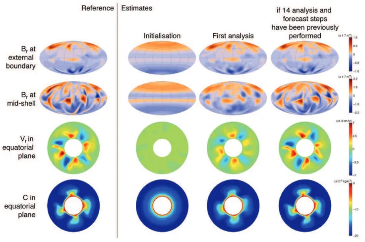
Fig. 3. Results of a twin experiment with model 1, where the surface radial magnetic field (first line) and its secular variation (not shown),

both given up to degree and order 13, are used to retrieve the internal structure (second to fourth line). Column 1 is the state of the reference at timet=1.3τsec. Column 2 is the assimilation state if only the initialisation step has been performed at timet(it thus represents the time

average of the simulation, see Table 2). Column 3 is the assimilation state if only the initialisation step and the first analysis step as been performed at timet. Column 4 is the assimilation state if it has been initialised at timet=0, and if 14 analyses and forecast steps have been subsequently performed with a time lag 0.1τsec(about 50 yr in Earth time) until timet=1.3τsec(note that this column then represents the

forecast, not the analysis). For this run we usedβ=0.75. All fields are presented in the units proposed in Sect. 2.2, with their tentative rescaling to Earth’s core values in parentheses.

run computation used to build P. The internal structure esti-mates are thus worse in the vicinity of this statistical outlier. The fact that the recovery quality fluctuates stands in trast with the ideal Kalman filter which, when used in con-junction with a linear model and when updating a properly initialized error covariance matrix of the model, statistically reduces the misfit between the recovery and the reference (see e.g. Fournier et al., 2010). Our assimilation scheme loses this property because of its imperfections: a time-independent covariance matrix is used and a part of the so-lution length scales spectrum (forlandmabovelmaxp ) is left untouched at analysis time and remains only determined by the dynamics. These uncorrected, dynamically determined scales tend to backreact on the other scales through the non-linear couplings present in the dynamical equations, thus di-verting the system trajectory away from the reference. The fluctuating recovery quality is then the result of a balance

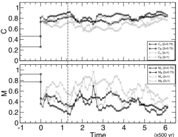
0 0.2 0.4 0.6 0.8 1 C

Cu (β=0.75) CB (β=0.75) Cu (β=1) CB (β=1)

-1 0 1 2 3 4 5 6

Time 0 0.2 0.4 0.6 0.8 1 M

Mu (β=0.75) MB (β=0.75) Mu (β=1) MB (β=1)

(x500 yr)

Fig. 4. Correlation and misfit coefficients after analysis, for the same series of twin experiments as in Fig. 3, for whichβ=0.75

(black), and for a similar series whereβ=1 (grey). Time is in

units ofτsec, as detailed in Sect. 2.2, with a tentative rescaling in

real time in parentheses. The assimilation is initialised and first analysed at timet=0, the values ofMandCreported at negative times are those obtained between the first reference sample and the model time average (which is the initialisation step estimate, second column of Fig. 3). The vertical dashed line is the time at which the fourth column of Fig. 3 has been obtained.

experiments with variable noise levels added to the obser-vations (not shown here) show that the benefits of setting

β=0.75 are preserved when observations are imperfect. To illustrate the issue of observed, estimated and dynami-cally determined scales, we next focus on energy spectra of the surface magnetic field (Fig. 5). Since the data are con-sidered perfect, performing an analysis always results in a perfect match between the observed part of the system and the observations, as illustrated by the vanishing residual be-tween the spectra of the analyses and the reference up to de-gree 13. The first analysis (red curve in Fig. 5) uses the cor-relations contained in P to additionally estimate the unob-served surface field coefficients between degree 14 and de-greelmaxp =15. Coefficients with degrees larger thanl

p maxare not estimated by the first analysis. In contrast, the 15th anal-ysis (green curve, performed immediately after the forecast presented in the fourth column of Fig. 3) benefits from a dy-namical determination of these coefficients, and reduces the misfit to the reference by a factor of 2 for harmonic degrees between 15 and 30.

An important aspect of data assimilation is the evaluation of the forecast quality. When dealing with a real system, it is indeed impossible to evaluate the recovery quality of the internal structure as it was done in Fig. 4. It is however pos-sible to use surface data in order to evaluate a-posteriori how well the system has predicted a given time evolution. This

0 10 20 30 40 50 60

harmonic degree

10-6

10-4

10-2 Ref-1st

Ref-15th 10-6 10-4 10-2

Energy

observed scales dynamically determined scales Estimated scales

Fig. 5. Top: energy spectra of the magnetic field at the model

sur-face for the reference solution (black), the first analysis (red) and the 15th analysis (green). The procedure through which these anal-yses are obtained is described in Fig. 3. Bottom: energy spectra of the differences between the reference, the first and the 15th analy-ses. Units as described in Sect. 2.2, with their tentative rescaling in parentheses.

provides a combined assessment of the performance of the assimilation scheme, of its possible biases and of the suit-ability of the model for describing the real system (dealing with synthetic data, our study does not cover this last as-pect). The quality of thei-th forecast xf_i can only be assessed from the standpoint of the observer and its limited access to the system. It is thus evaluated on the observed part of the system only, using the instantaneous innovation (or instan-taneous forecast error) vector di=yi−Hx

f

i (which indeed

represents the difference between the observable part of the forecast and the data), or more precisely through its norm

di= ||di||. (21)

Here our norm definition is adapted such that each harmonic coefficient is multiplied withl(l+1)/ro prior to the

evalu-ation of the norm, such that the result is a rms value of the radial magnetic field at the outer boundary (or its time deriva-tive). One important property of the innovation vector di is

that its statistical expected value should be zero for an unbi-ased assimilation scheme (e.g. Talagrand, 2003). Computing the cumulative mean innovation

dk=

1 k k X

i=1 di (22)

0

5

10

15

10

10

10

10

10

10

10

instantaneous cumulative mean (x1.7 mT)

(x500 yr)

overturn time

Innovation

overturn time

0.01 τsec

0.05 τsec

0.1 τsec

0.2 τsec

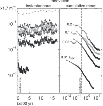
Fig. 6. Instantaneous innovation (or instantaneous forecast error)

di and cumulative mean innovationdkas a function of assimilation

time, for the sequence presented in Fig. 3 and other sequences with same access to observable quantities and assimilation parameters but varying forecast horizon (which is the same as the time lag be-tween analyses), from 0.01τsecto 0.2τsec(solid black lines, each

circle represents an analysis, forecast horizon increases vertically). The innovation is computed only with the magnetic field (not the secular variation). Also plotted are an assimilation sequence with β=1 (solid grey line, forecast horizon 0.1τsec) and the root-mean

squared radial magnetic field amplitude at the outer boundary for the reference sequence (dashed line). Units as in previous figures.

comprises the poloidal magnetic field up to degree and or-der 13 and its secular variation up to a variable degree and order (13 in the case of Figs. 3 to 6). However, to facili-tate comparison between sequences where secular variation is assimilated to a variable degree (see Fig. 7 below), we will evaluate the forecast quality only on the observed magnetic field poloidal coefficients up to degree 13. As expected from the discussion of Fig. 4,didoes not decrease with the number of assimilation cycles, but oscillates about a slowly increas-ing baseline. This long-term trend does not mean that the assimilation gets worse over time, but is simply the conse-quence of an increase of the reference seconse-quence magnetic en-ergy through time (dashed line in Fig. 6). In line with Fig. 4,

di is significantly reduced when β is decreased from 1 to

0.75. Regardless of the forecast horizon (which is the same as the time lag between analyses),dk decreases sharply

af-ter one system overturn time (which is about 0.3 in units of

τsec, a value which is quite independent of the chosen model, Christensen and Tilgner, 2004; Lhuillier et al., 2011a). At very long assimilation times,dkceases to decrease, revealing

the existence of a forecast bias in our scheme. The bias sig-nificantly decreases whenβis decreased from 1 to 0.75. This shows that it is connected to the influence of the uncorrected variables of the state vector on the corrected variables. Al-though it would certainly be desirable to implement a bias re-moval strategy in the assimilation scheme, the present bias is not likely to be a limiting factor in practical applications, its level being typically one order of magnitude lower than the intrinsic forecast error introduced by the assimilation. Fur-thermore, long assimilation times (here 8500 yr) are needed to reveal the presence of this bias. Our synthetic experi-ments, where high-quality data are assimilated in such long sequences, obviously do not represent a practical situation, given the presently available record of Earth’s magnetism on centennial to millenial timescales (e.g. Hulot et al., 2010a).

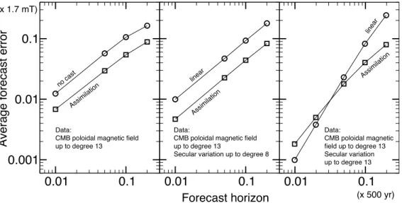
To really become meaningful, the absolute forecast quality should be compared to that obtained with other prediction strategies, the simplest of which is the “no-cast”, or use of the present magnetic field as a forecast for the future. Another still simple strategy is the linear extrapolation of the existing surface magnetic field, making use of the secular variation data. The results of series of no-casts, linear extrapolations and assimilations are reported in Fig. 7, for various forecasts horizons never exceeding the systeme-folding time 0.6τsec. The average forecast error is defined as

d= 1 na

na X

1

di, (23)

wherenais the total number of assimilation cycles. The aver-age forecast errord should not be confused with the cumula-tive mean innovation,dk. It can be first noted thatd

0.01

0.1

Forecast horizon

0.001

0.01

0.1

Average forecast error

0.01

0.1

0.01

0.1

no cast

Assimilation

Assimilation

Assimilation

linear

linear

Data:

CMB poloidal magnetic field up to degree 13

Data:

CMB poloidal magnetic field up to degree 13

Secular variation up to degree 8

Data:

CMB poloidal magnetic field up to degree 13 Secular variation up to degree 13

(x 1.7 mT)

(x 500 yr)

Fig. 7. Average forecast errordof surface poloidal magnetic field coefficients up to degree and order 13, for various prediction strategies and variable forecast horizon. From left to right: the no-cast (poloidal magnetic field coefficients up to degree 13 at a given time are used to forecast at a later time), the linear forecasts (poloidal magnetic field coefficients (B) up to degree 13 and secular variation (SV) up to degree 8 or 13 are used for a linear extrapolation) are compared with the assimilation using the exact same amount of data. For each panel, the average forecast error is computed on an equal number of cycles for the assimilation and the linear prediction. All sequences haveβ=0.75 as in Fig. 3. Units as in previous figures. The averaging time interval for all sequences presented in this figure is from 0 to 6τsec.

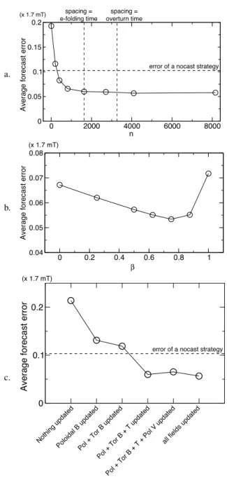
In a final series of experiments (Fig. 8), we use the fore-cast quality as an indicator to perform a number of checks on our data assimilation framework. The first of these is an evaluation of the adequate numbernof free run snapshots needed for building a robust estimate of P, as well as their spacing. Figure 8a shows that more than 1000 samples with a spacing at least equal to thee-folding time of the system are needed for a reasonable determination of the covariance matrix. Conversely, using a too small set of samples leads to forecast errors which may exceed the error made with a no-cast strategy. The next test evaluates the impact of the factorβ which controls the amount of correction brought by the data at analysis time. Figure 8b shows that an optimum in the forecast quality is reached forβ=0.75, which underlines again the potentially deleterious effect of re-injecting all the dynamically determined scales into the system after analysis. Re-injecting some of these dynamically determined scales is however beneficial to the forecast quality, as seen from the regular decrease of the average error fromβ=0 toβ=0.75. Finally, we have performed experiments (Fig. 8c) where the correction at analysis time has been turned off for one or sev-eral fields. Obviously, correcting only the magnetic field har-monic potentials results in a better forecast than not assimi-lating anything, but the forecast quality will outperform that of a no-cast strategy only if the flow and buoyancy harmonic potentials are also corrected. Note that the best improvement comes from updating the buoyancy potential, presumably be-cause the flow driven by the buoyancy anomaly is then also well estimated. This last test emphasizes the benefit of using

multivariate statistics for the estimation, and also illustrates the difficulties encountered by monovariate, modelled co-variances (Kuang et al., 2009) in forecasting the field with better accuracy than that of a linear extrapolation.

3.3 Synthetic inversion tests, model 2

The satisfying results obtained with model 1 can be under-stood through the strong linear couplings existing between the observed and unobserved part of the system. To eval-uate the impact of stronger nonlinearities, we now turn to synthetic experiments performed with model 2. Following the prescriptions obtained through the analysis of model 1, the co-variance matrix for model 2 was built usingn=978 samples in the free run, with a spacing between samples of 0.125τsec, which is about three times longer than the sys-tem e-folding timeτe=0.04τsec. The duration of the free run is 0.65 magnetic diffusion times or 122τsec, amounting to 61 000 yr ifτsec=500 yr. It should be noted from Fig. 8 that if we were to usen=978 also in model 1, this would not substantially degrade the quality of the inversions. The differences present in the following results should thus not be ascribed to the size of the error space (which is the rank of the covariance matrix and is equal ton). The matrix coefficients were computed up to degree and orderlP_max=30. All assim-ilation experiments have been performed usingβ=0.75.

a.

0 2000 4000 6000 8000 n

0 0.05 0.1 0.15 0.2

Average forecast error

error of a nocast strategy spacing =

e-folding time

spacing = overturn time (x 1.7 mT)

b.

0 0.2 0.4 0.6 0.8 1

β

0.04 0.05 0.06 0.07 0.08

Average forecast error

(x 1.7 mT)

c.

Nothing updated

Poloidal B updated_{Pol + Tor B updated} Pol + Tor B + T updated

Pol + Tor B + T + Pol V updated all fields updated 0

0.1 0.2

Average forecast error

error of a nocast strategy (x 1.7 mT)

Fig. 8. Average forecast errordfor series of experiments where the surface magnetic field is assimilated up to degree 13 (the sec-ular variation is not assimilated here), and the forecast horizon is 0.1τsec. (a) the factorβis set to 0.75 and the numbernof

sam-ples used to build P is varied by decimating an ensemble of 8155 snapshots obtained during the model free run, the spacing between each snapshot being 0.13τsec. Two vertical dashed lines indicate

the values ofnfor which the spacing between snapshots is equal

to thee-folding and overturn times of the system. (b) The number

nof samples is set to 4098 and the factorβis varied from 0 (the system is reset to its time average state prior to each analysis) to 1 (the analysis is performed on the forecast resulting from the previ-ous time integration). (c) The correction at analysis time has been turned off for some, or all fields (n=4098,β=0.75). Same time averaging interval as in previous figure.

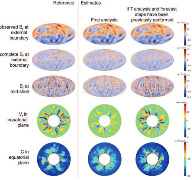
surface magnetic field was observable). With the exception of this additional line, all other lines have the same color bars as the corresponding lines of Fig. 3, in order to high-light the relevance (and possible shortcomings) of the scaling procedure which we have adopted (see Sect. 2.2). From an order-of-magnitude standpoint, the rescaling is indeed satis-factory, but there are variations within the order of magni-tude which the scaling theory fails to describe. For instance, model 2 has a slightly larger internal magnetic energy than model 1 (third line of Fig. 9) but less magnetic flux escapes at the surface (second line). The large-scale velocity and buoyancy anomaly fields have roughly the same amplitude as in model 1, but more powerful small-scales, located mostly within the strong plumes emerging from the inner boundary. When compared to model 1, the static stochastic inversion of one data sample (second column of Fig. 9) captures less of the internal structure of the dynamo. The system is in-deed less observable, in the sense that a reduced state vector which is now ten times larger (see Table 1) needs to be con-strained by the same amount of observation. Furthermore, the stronger nonlinearities present in model 2 tend to even out correlation peaks resulting from the linear couplings in the covariance matrix of model 2, resulting in less accurate estimations. Still, at the exception of the deep magnetic field (third line), which is too small-scaled to be well constrained by the surface observations (first line), a number of gross de-tails of the internal solution are retrieved. The first estimate is underpowered as it was for model 1. If more data samples have been previously assimilated through integration of the time evolution scheme (third column), the estimate reaches the same power as the reference. After a time of 0.7τsec (corresponding to about two overturns), the deep fields are only qualitatively recovered in a morphological sense. The gross details of the convection flow and thermal plumes are roughly into place. However, small scale details created by the nonlinear dynamics, which are especially prominent in the deep magnetic field map, are clearly not constrained by the surface observations and the scheme. The frozen co-variance matrix which we have obtained for model 2 lacks the ability to reliably estimate small-scale details from the large-scale observations. Indeed we have seen in Sect. 3.1 that couplings between different harmonic orders are non-existent, and that couplings between harmonic degrees are prominent under the condition that the solution is rather well controlled by the linear part of the equations (including the Coriolis force). The strong nonlinear dynamics is thus left free to populate these small-scales in a rather unconstrained way. This deleterious effect is also enhanced by the fact that the size of the uncorrected part of the state vector is ten times larger in model 2 when compared to model 1 (Table 1).

Fig. 9. Results of a twin experiment with model 2, where the surface radial magnetic field (first line) and its secular variation (not shown),

both given up to degree and order 13, are used to retrieve the internal structure (second to fifth line). The first column is the reference. Similarly to Fig. 3, column 2 is the estimate if only the initialisation and the first analysis steps have been performed, and column 3 is the estimate obtained after performing a full data assimilation sequence where 7 data samples spaced 0.1τsectime units each are injected in the

model. Note that for this last column, the state of the system is represented after the forecast (not after the analysis). For this run we used β=0.75. For comparison purposes, units and color bars for lines 2 to 5 are the same as in Fig. 3.

Fig. 7, the error for the various strategies no longer follow a power-law of the forecast horizon as this horizon approaches the systeme-folding timeτe=0.04τsec. Indeed it is expected (Hulot et al., 2010b; Lhuillier et al., 2011a) that the error starts to become of macroscopic (same order of magnitude as the reference) amplitude beyond this point, as confirmed by our experiments. The left panel of Fig. 10 shows that the assimilation never performs significantly better than the no-cast. Moreover, when secular variation data up to degree 13 are also used, the linear extrapolations are shown to be much better than the assimilation forecasts, for all horizons below thee-folding time where both strategies again yield the same error. Given thatRe=858 for model 2, the secular variation

at the outer boundary is now mostly controlled by flow ad-vection underneath the outer boundary. The flow responsible for the secular variation is nonlinearly coupled to the obser-vations, and thus not well grasped by our linear estimation technique. This explains the worse results obtained by the assimilation.

0.01 0.1

0.01 0.1

0.001 0.01

Forecast horizon

Average forecast error

(x 1.7 mT)

(x 500 yr) no cast

Assimilation

Assimilation

linear

τe τe

Data: CMB poloidal magnetic field up to degree 13

Data: CMB poloidal magnetic field up to degree 13 Secular variation up to degree 13

Fig. 10. Average forecast errordof surface poloidal magnetic field coefficients, for model 2, various prediction strategies and various forecasts horizons, computed as in Fig. 7.

such low error analyses, this reduces the prospect of im-plementing a reasonably complex and realistic geomagnetic data assimilation framework in an operational context. How-ever, assuming that the errors of the assimilation and linear extrapolation strategies are decorrelated, and if their statistics are known, the predictions from both strategies can be com-bined in order to provide a third prediction which is better than the two original ones. Such an additivity of accuracies is a concept at the root of the linear estimation theory. Here again, a Kalman filter is the adequate tool to perform this task. If we assume that we can estimate the error covariance matrix R of linear extrapolations, and if, for a given forecast horizon, we have both the linear extrapolation forecast xf l and the assimilation forecast xf, then the combined forecast xf cis such that

xf c=xf+K(Hxf l−Hxf). (24) In a more readable presentation which involves the observ-able parts yf l=Hxf l, yf =Hxf and yf c=Hxf c, and the model covariance matrix reduced to the observable part O=

HPH′_{, the combined forecast writes:}

(O+R)yf c=Oyf l+Ryf. (25)

The combined forecast is thus simply an optimal interpola-tion of the two other forecasts. Figure 11 illustrates this con-cept on a forecast horizon 0.05τsec, roughly equal to the sys-tem e-folding time. Diagonal coefficients of the matrix R (Fig. 11a) are estimated following the same procedure as in Sect. 3.1, using 100 linear forecasts performed in a prelimi-nary run of the model. Cross-correlations in the error statis-tics are neglected (non diagonal coefficients are set to 0). Er-rors are naturally statistically centered, and according to the formalism outlined in Sect. 2.3, they are normalised with the corresponding diagonal variances used for P. An error equal

a

0 50 100 lm 0

0.2 0.4 0.6 0.8 1

Rlm,lm

free run variance

b

0 0.2 0.4 0.6 0.8 1

Time 0.01

0.02

innovation _{Assimilation forecasts}

linear forecasts optimal interpolation of the two

(x 500 yr) (x 1.7 mT)

Fig. 11. (a): empirically-estimated diagonal coefficientsRlm,lmof

the error covariance matrix R for linear forecasts of model 2 at the horizon 0.05τsec. Coefficients are normalised with the

correspond-ing variances of the free run, and are ordered accordcorrespond-ing to the same

one-parameterlmordering scheme as in Fig. 2. Non-diagonal

coef-ficients are set to 0. (b): instantaneous innovation (or instantaneous forecast error)di (circles) for the assimilation sequence shown in

Fig. 9 with forecast horizon 0.05τsec. Also represented are the

re-sults of a linear extrapolation using the exact same amount of data, i.e. the surface magnetic field and secular variation coefficients up to degree 13 (squares), and the results of a combined forecast (dia-monds) as defined in Eq. (25), using the empirically-estimated ma-trix R.

to one thus means that the linearly forecast harmonic coeffi-cient varies as much as what was observed for the coefficoeffi-cient itself during the model free run. From Fig. 11.a it appears that the linear forecast performs better on large scales than on small scales. The optimal interpolation outlined above has the effect to mitigate this error by injecting more of the assimilation forecast when the linear forecast error is large. The overall root-mean-squared forecast error thus decreases (Fig. 11b). The quality of the combined forecast outperforms that of the linear extrapolation by about 10 %, and that of the assimilation by about 40 %. More importantly, the combined forecast is shown to be always better than the best of the two strategies. This clearly underlines the interest of hav-ing several independent prediction strategies at hand when attempting to perform forecasts, especially if each strategy is far from perfect.

4 Discussion

a sequential assimilation scheme, can provide inferences on the internal structure of numerical dynamos from surface ob-servations only. The way the stochastic inverse handles the non-uniqueness problem is through the use of prior informa-tion, obtained by directly computing the multivariate statis-tics of the numerical models from a suitably large set of snap-shots with enough spacing between each other. Strong corre-lations were found between the surface observations and the internal fields, which arise from the linear part of the dynam-ical equations and the leading influence of the Coriolis force in the dynamics. This led to excellent synthetic recovery results with a weakly nonlinear model (model 1). Stronger nonlinearities (model 2) however defeat the linear estimation technique to some extent, even though nonlinearity itself can be used with some success in estimating the part of the under-lying field spectrum which is neither observed nor correlated to surface observations (Fig. 5). This could provide a possi-ble path towards improving spatial resolution propossi-blems of the existing inversion strategies mentioned in the introduction.

With kinematic Reynolds numbers of order 109and mag-netic Reynolds number of order 103 (e.g. Christensen and Tilgner, 2004; Aubert et al., 2009) it is certain that nonlinear-ities are important in Earth’s core dynamics. Our results are encouraging but highlight the need for estimation techniques specifically designed to handle a large amount of nonlinear-ity. When dealing with such magnetic Reynolds number (as is the case in model 2), advection by the flow underneath the outer boundary is responsible of most of the secular vari-ation in the observed range. The linear estimvari-ation of core flow performed in this study is clearly insufficient and could be replaced by a classical inversion of the radial induction equation (see for instance Finlay et al., 2010a), which han-dles the nonlinear nature of core flow advection correctly. Another important point is to implement a time evolution al-gorithm for the model covariance matrix, in order to have an instantaneous matrix which, for each analysis time, should be more adapted to the evaluation of nonlinear correlations than the generic, frozen covariance matrix in which, as we have seen, only the correlations subsequent to the linear part of the system arise. A promising method is for instance the ensemble Kalman filter (Evensen, 1994), where the model er-ror statistics are evolved through the use of an ensemble of models states created around the actual model trajectory with the help of a Monte-Carlo method. Such a method is how-ever much more costly in terms of computer power than the method which we have presented here, which had require-ments on disk space (400 GB for model 2) and random ac-cess memory (30 GB) only at the time of the computation of the frozen model covariance matrix.

Geomagnetic data assimilation is however still in its in-fancy, and more acute problems need to be solved before geomagnetism can integrate the advanced data assimilation techniques routinely used in atmospheric and ocean sciences. One of these issues is the choice of a numerical model for performing an operational inversion for the internal structure

of the geodynamo. As discussed in the introduction, the Earth’s core has an extraordinary disparity in the diffusivi-ties of the involved fields, as measured for instance by the magnetic Prandtl number P m≈10−6 of liquid iron. Nu-merical models are not able to handle such diffusivity con-trasts and operate at Prandtl numbers close to unity. Even if we can reach an acceptable level of magnetic turbulence (Rm=O(1000)), current computer power limitations make it impossible to reach a level of hydrodynamic turbulence which approaches that of the Earth’s core. As a result, even if the magnetic induction phenomenon is correctly simulated, we should be cautious about the relevance of the large-scale velocity output of our simulations and inversions. In the ab-sence of a clear path towards improving this situation, our understanding of the physical grounds underlying the mor-phological semblance between numerical dynamos and the geomagnetic field (Christensen et al., 2010) suggests that we should select a model which has the lowest possible ratio between the length of the day and the magnetic dissipation time scale (the magnetic Ekman number) and a ratio between the magnetic advection and diffusion time scale approaching 1000 (the magnetic Reynolds number). In that sense model 2 should be much better suited than model 1 for the task of inverting real geomagnetic data, but here a trade-off should be made between the physical relevance of the model and the ability to linearly estimate hidden state variables, which, as we have seen, is precisely hampered by the fact that the magnetic Reynolds number is large.

It is interesting to briefly review how geomagnetic data as-similation strategies currently in development deal with the issue of this improper rendering of the real physics. Kuang et al. (2010) propose that these modelling errors evolve on a time scale longer than that at which observation data can be made. In that case they can be mitigated by per-forming two closely spaced assimilation sequences. The method is promising and already resulted in a secular vari-ation model for the latest genervari-ation of the IGRF (Finlay et al., 2010b). It is however limited to surface field forecast-ing activities. Progress in determinforecast-ing the internal dynamical structure could be achieved through combining data assimi-lation with asymptotic assumptions on core dynamics, for in-stance the quasi-geostrophic assumption (Canet et al., 2009), or building Taylor states (Livermore et al., 2010) compatible with surface observations. In any case, using several inter-nal structure modelling approaches within their spatial and temporal range of validity could help overcome the intrinsic limitations of each strategy. For instance, a quasi-geostrophic framework is more appropriate for rapid (decadal) flow vari-ations (Jault, 2008) while a three-dimensional numerical dy-namo is suitable for describing long-term, ageostrophic flows such as thermal winds (Aubert et al., 2010).