www.ann-geophys.net/28/2079/2010/ doi:10.5194/angeo-28-2079-2010
© Author(s) 2010. CC Attribution 3.0 License.
Annales
Geophysicae
Averaging and sampling for magnetic-observatory hourly data
J. J. Love1, V. C. Tsai2, and J. L. Gannon1
1Geomagnetism Program, US Geological Survey, Denver, CO, USA 2Earthquake Hazards Program, US Geological Survey, Denver, CO, USA
Received: 21 May 2010 – Revised: 25 October 2010 – Accepted: 5 November 2010 – Published: 12 November 2010
Abstract.A time and frequency-domain analysis is made of the effects of averaging and sampling methods used for con-structing magnetic-observatory hourly data values. Using 1-min data as a proxy for continuous, geomagnetic variation, we construct synthetic hourly values of two standard types: instantaneous “spot” measurements and simple 1-h “boxcar” averages. We compare these average-sample types with oth-ers: 2-h average, Gaussian, and “brick-wall” low-frequency-pass. Hourly spot measurements provide a statistically unbi-ased representation of the amplitude range of geomagnetic-field variation, but as a representation of continuous geomagnetic-field variation over time, they are significantly affected by alias-ing, especially at high latitudes. The 1-h, 2-h, and Gaussian average-samples are affected by a combination of amplitude distortion and aliasing. Brick-wall values are not affected by either amplitude distortion or aliasing, but constructing them is, in an operational setting, relatively more difficult than it is for other average-sample types. It is noteworthy that 1-h average-samples, the present standard for observatory hourly data, have properties similar to Gaussian average-samples that have been optimized for a minimum residual sum of amplitude distortion and aliasing. For 1-h average-samples from medium and low-latitude observatories, the average of the combination of amplitude distortion and aliasing is less than the 5.0 nT accuracy standard established by Intermag-net for modern 1-min data. For medium and low-latitude observatories, average differences between monthly means constructed from 1-min data and monthly means constructed from any of the hourly average-sample types considered here are less than the 1.0 nT resolution of standard databases. We recommend that observatories and World Data Centers con-tinue the standard practice of reporting simple 1-h-average hourly values.
Keywords. Electromagnetics (Measurement and standards)
Correspondence to:J. J. Love ([email protected])
1 Introduction
Since magnetic observatories first began operating around the world in the middle of the 19th century, one of their most important products has been hourly data values. Historical hourly observatory data are useful for a variety of applica-tions (e.g. Parkinson, 1983; Courtillot and Le Mou¨el, 1988; Barraclough et al., 1992; Pr¨olss, 2004), including studying geomagnetic secular variation originating in the core (e.g. Sabaka et al., 2004), exploring the electrical conductivity of the mantle (e.g. Egbert et al., 1992), mapping electric cur-rents in the ionosphere (e.g. Campbell, 1989), measuring the intensity of magnetospheric storms (e.g. Karinen and Mur-sula, 2005), and estimating long-term solar-terrestrial inter-action (e.g. Macmillan and Droujinina, 2007). In conducting these, and other types of analyses, it is important, and some-times even essential, to have an understanding of the effects of amplitude distortion and aliasing caused by averaging and sampling procedures used in the production of hourly data.
or, more formally, they were calculated from multiple sub-hour spot measurements. The switch from making spot mea-surements to producing average values came gradually: in Great Britain (Eskdalemuir) it was made in 1912 (Meteoro-logical Office, 1914, p. 68), in the United States at all ob-servatories in 1915 (e.g. Hazard, 1918, p. 5), and at some observatories in France (Chambon la Forˆet) not until 1972 (Fouassier and Chulliat, 2009, p. 87). Today, constructing hourly means is done by computer, averaging digital 1-min data acquired by electronic systems.
Because the historical hourly observatory data are a mix-ture of spot measurements and hourly averages, their prop-erties have changed over time, and their time series can be described as being “inhomogeneous”. Spot sampling can sometimes, and fortuitously, give a good record of short-duration transient magnetic-field variation. Spot sampling can also sometimes, and unfortunately, miss transient varia-tion altogether. It all depends on when and how frequently samples are taken relative to when and over what duration the field variation occurs. If we assume, as is reasonable, that spot measurements are collected independently of field variation, then numerous spot measurements collected over a long period of time will represent an unbiased statistical sampling of the amplitude range of magnetic-field variation. On the other hand, averaging reduces the amplitude of high-frequency variation, giving a time series that is smoother than actual magnetic-field variation. The statistical variance of discrete 1-h-average values will be less than that of the mag-netic field’s actual variation, and it will be less than that of in-stantaneous, spot measurements. Since magnetic-field vari-ation occurs over an extremely broad range of frequencies, discrete hourly sampling, be it done with spot measurement or with an averaging window, will result in aliasing, with high-frequency amplitudes being mapped into estimates of low-frequency amplitudes.
Researchers often use a combination of spot and hourly-average observatory data, as if, together, they represent a reliable long-term record of magnetic-field variation. It is, therefore, natural to ask: can we measure differences in the properties of hourly spot and hourly average values so that informed decisions can be made about using them? How do spot and hourly averages compare with other hypothetical average-sample types that might be proposed in the future as candidate observatory products? In seeking answers to these and other related questions, we examine the properties of hourly observatory data, measuring their variance, relative proportionality, correlation, autocorrelation, spectral power, amplitude distortion, and aliasing. Assuming that 1-min data are a good representation of continuous magnetic-field varia-tion, we construct several types of synthetic hourly average-samples from 1-min data collected from observatories situ-ated at different latitudes. We employ standard methods of continuous (e.g. Bracewell, 1978; Kanasewich, 1981) and statistical (e.g. Lee, 1960; Bendat and Piersol, 2000) time-series analysis.
2 Data
In Table 1 we summarize the data we use. The 1-min data are definitive (processed and calibrated) magnetic-vector val-ues collected at observatories (Jankowski and Sucksdorff, 1996; Love, 2008) that meet Intermagnet standards (Ker-ridge, 2001; Rasson, 2007); we obtained the 1-min data from the Intermagnet website (www.intermagnet.org) for observa-tories situated at high (Barrow BRW), medium (Chambon la Forˆet CLF), and low (Huancayo HUA) geomagnetic lat-itudes. They record a variety of magnetic-field variation, with high (low) latitude variation dominated by active au-roral (equatorial) electrojets (e.g. Parkinson, 1983; Pr¨olss, 2004), and medium-latitude variation being relatively more quiescent. Each 1-min magnetic-vector datum was formed from sub-minute electronic signals acquired from a tri-axial fluxgate magnetometer. The signals were both analog and digitally filtered, effectively eliminating aliasing from vari-ation with periods of less than 1-min (frequencies greater 0.0167 Hz). Additional measurements, made once a week or so from a reference pier at each observatory site, were combined with the fluxgate measurements to construct time series that have an accuracy, measured in absolute terms over many years, of better than 5.0 nT (0.50′). Each 1-min datum has a time stamp that is centered on the top of the universal-time (UT) minute (HR:MN:SC, 00:00:00, 00:01:00, etc.). For BRW and HUA, we use almost a complete solar cycle of data (1998.0–2009.0), and for CLF we use almost two so-lar cycles of data (1991.0–2009.0).
Table 1.Summary of observatories and data used. Geomagnetic latitudes are calculated for a 2005 dipole.
Code Observatory name Region Data used Years Geomag. Lat. Present supporting institute BRW Barrow Alaska min Intermagnet 1998.0–2009.0 69.6◦ US Geological Survey
CLF Chambon la Forˆet France min Intermagnet 1991.0–2009.0 49.8◦ Institut de Physique du Globe de Paris HUA Huancayo Per´u min Intermagnet 1998.0–2009.0 −1.8◦ Instituto Geofisico
CLF Chambon la Forˆet France h WDC-CE 1954.0–1990.0 49.8◦ Institut de Physique du Globe de Paris ESK Eskdalemuir Britain h WDC-CE 1917.0–1947.0 57.8◦ British Geological Survey
differences between hourly spot samples and 1-h averages. We use the ESK-CE data to investigate the effects of heavy averaging.
For both the 1-min data and hourly values, we use geographic-polar (horizontalH, declinationD, verticalZ) magnetic-vector components. When these are the com-ponents in the WDC database, then we use them without any modification, otherwise, if and when cartesian (north X, east Y) horizontal components are reported, then we calculate (D,H ) appropriately. Data spikes are identified with a simple computer algorithm; these are removed and, along with occasional data gaps, filled with interpolated val-ues. The British Geological Survey’s annual-means database (www.geomag.bgs.ac.uk) contains a list of small step-offsets in the historical time series; some are also documented in ob-servatory yearbooks. Most step offsets are obvious from in-spection of the data; they are the result of moving the obser-vatory’s reference pier, changes in measurement method, or uncontrolled contamination. We insert complementary step-offsets into the historical observatory time series in order to bring them into continuity. The details of these adjustments do not significantly affect the results that follow.
3 Theory
The standard averaging and sampling methods that are used for constructing observatory hourly values are mathemati-cally equivalent to passing a continuous magnetic-field time series through a zero-phase-delay linear filter, and, then, dis-cretely sampling the output once per hour. In this section of mathematical review, we examine the properties of different averaging and sampling types in the dual domains of time and frequency. The average-samples are simple, and they in-clude the standard spot and 1-h averages used for construct-ing hourly values, as well as other average-sample types use-ful for comparison.
yearbooks record data in XY Z coordinates, but the pre-1932.0 WDC-CE holdings are inH DZ coordinates – another indication that the data were manipulated at some point after first reporting. Furthermore, the pre-1932.0 ESK digital holdings of WDC Kyoto are different from those of WDC-CE. Indeed, the WDC-K data ap-pear to be close to the original yearbook data, but there are some formatting problems with the WDC-format version of the ESK-K data.
For notation, we represent the time series of an arbitrary magnetic-vector component asB(t ), which is a function of timet, and which can stand for any ofH (t ),D(t ),Z(t ), etc. We assume thatB(t ) is well behaved: it is finite, continu-ous, and integrable. These qualities pertain to any natural magnetic-field time series measured over a finite duration of time and that might be generated from classical physical processes. Therefore, once the data have been detrended, a Fourier-type analysis can be reasonably pursued. We use a Fourier transformationF having a “unitary” normalization for ordinary frequenciesf, wheret=1/f. For a signalB(t ) in the time domain, its dual in the frequency domain,B(f ),˜ is given by
˜
B(f )=F{B(t )} = Z +∞
−∞
B(t )e−2πif tdt. (1) Inverse Fourier transformation is given by
B(t )=F−1{ ˜B(f )} = Z +∞
−∞
˜
B(f )e2πif tdf. (2) The unitary normalization is used in the classic textbook by Bracewell (1978, p. 6); it is different from the non-unitary normalization for angular frequencies used by Lee (1960, p. 33). In most respects, this is a technical distinction, one that does not affect a qualitative understanding of the theory and results that follow.
3.1 Simple running averaging
We begin by considering the straightforward running aver-age of a geomagnetic time series. With a rectangle-in-time or “boxcar” function, simple averaging is defined over a du-ration of timetaby convolution of
rect(t;ta)≡
1 |t|< ta/2
0 |t|> ta/2 (3) with the natural, continuous magnetic-field time seriesB(t ), Ba(t )=
1 ta
B(t )∗rect(t;ta) (4) = 1
ta Z +∞
−∞
B(ζ )rect(t−ζ;ta)dζ
= 1 ta
Z t+ta/2
t−ta/2
Fourier transformation of the rectangle function in the time domain is a sinc function in the frequency domain,
1 ta
F{rect(t;ta)} =sin(πf/fa) πf/fa ≡
sinc(f;fa) (5) (Bracewell, 1978, p. 389), wherefa=1/ta.
By the convolution theorem (Lee, 1960, p. 28; Bracewell, 1978, Ch. 3), the Fourier transform of convolution in the time (frequency) domain is equal to multiplication in the fre-quency (time) domain,
F{B(t )∗rect(t;ta)} =F{B(t )}F{rect(t;ta)}. (6) With this,
F{Ba(t )} = ˜Ba(f )= ˜B(f )sinc(f;fa), (7) whereB(f )˜ is the frequency-domain dual ofB(t ). The func-tion sinc(f;fa)gives the mapping fromB(f )˜ toB˜a(f ); it is a “frequency-response” function (Bracewell, 1978, p. 179; Kanasewich, 1982, Ch. 5.3) that describes the amplitude dis-tortion of the time series in the frequency domain due to av-eraging. It is useful, now, to define the amplitude differences Aa(t )=B(t )−Ba(t ) and A˜a(f )= ˜B(f )− ˜Ba(f ), (8) which measure the signal in the original, continuous time se-ries that is not modelled by the running average. For a geo-magnetic reference to related issues, see Chapman and Bar-tels (1962, Ch. 16.17).
3.2 Low-pass brick-wall filtering
A low-pass “brick-wall” filter is most easily defined in the frequency domain (Bracewell, 1978, p. 52; Kanasewich, 1981, Ch. 15): it has a flat response below some chosen truncation frequencyfb/2, and it admits nothing above that frequency. Because the brick-wall filter has these proper-ties, it is sometimes described as “ideal”. It is prescribed by multiplication of the Fourier amplitudes by a rectangle-in-frequency function
˜
Bb(f )= ˜B(f )rect(f;fb), (9) and, correspondingly, by convolution in the time domain with a sinc function,
F−1nB˜b(f ) o
=Bb(t )= 1 tb
B(t )∗sinc(t;tb). (10) The difference between the original, continuous time series and the filtered time series is equal to unresolved frequencies abovefb/2,
Ab(t )=B(t )−Bb(t ) and A˜b(f )= ˜B(f )− ˜Bb(f ), (11) but there is no difference for frequencies belowfb/2.
Brick-wall filtering has two potential drawbacks. First, in the time domain, Bb(t )will show oscillations or “ringing”
near discontinuities or abrupt changes in the original, unfil-tered time seriesB(t )(Bracewell, 1978, p. 209; Kanasewich, 1981, p. 240). This is the Gibbs phenomenon. It is usually illustrated in textbooks by convolving a sinc function with a Heaviside step function; since the sinc function has oscilla-tory tails, the output of the convolution is also, to some de-gree, oscillatory. While natural geomagnetic time series have no discontinuities, they do sometimes record abrupt varia-tion, such as during storm sudden commencements. For this reason, the representation of a geomagnetic time series in terms of a brick-wall-truncated Fourier expansion will have ringing, which can be reasonably described as a Gibbs effect. But as we shall see, this does not significantly affect individ-ual hourly samples of a brick-wall-filtered time series.
The second potential drawback of brick-wall filtering con-cerns its practical implementation. In comparison to the other average-sample types considered here, it is relatively more difficult to use brick-wall filtering to obtain hourly val-ues. Accurate results require a long time series to be treated in the frequency domain. In contrast, simple boxcar aver-aging only requires one or two hours of data, and these can be treated in a straightforward way in the time domain; long time series are not needed to obtain accurate results. This simple point is especially relevant for institutes needing to promptly provide data for real-time operational applications. 3.3 Gaussian filtering
In the time domain, a Gaussian filter is defined as gaus(t;tσ)≡exp
−π t2/tσ2, (12)
for which time-domain convolution is given by Bσ(t )=
1 tσ
B(t )∗gaus(t;tσ). (13) The Fourier transform of a Gaussian is another Gaussian,
F{gaus(t;tσ)} = 1
fσgaus(f;fσ) (14)
(Bracewell, 1978, p. 386), wherefσ=1/tσ. In a qualita-tive sense, this time-frequency symmetry places the Gaus-sian filter midway between the two extremes of time-domain (frequency-domain) rectangle (sinc-function) filtering and sinc-function (brick-wall) filtering. The width of the Gaus-sian filter is specified bytσ, and, in Sect. 5.7, we will locate an optimal value. We note that Intermagnet recommends a Gaussian filter for the production of 1-min averages, but they do not make any similar recommendation for hourly values. 3.4 Spot sampling
For a constant sampling frequencyfs with discrete sample times
that are equally-spaced withtj+1−tj=ts=1/fs, we can de-fine a Dirac comb function as a sequence of equally-spaced delta functions,
comb(t;ts)≡ts X
j
δ(t−j ts)= X
j
δ(t /ts−j ) (16)
(Bracewell, 1987, p. 77; Kanasewich, 1981, pp. 34, 110). With this, instantaneous or “spot” sampling of a time series can be described as a multiplication of the original, continu-ous time series by the Dirac comb,
Bs(tj)=B(t )comb(t;ts)= (17) · · ·B(−2ts),B(−ts),B(0),B(+ts),B(+2ts),· · · (Bracewell, 1978, p. 78; Kanasewich, 1981, p. 35). Since the Fourier transform of a Dirac comb is another Dirac comb,
F{comb(t;ts)} = 1 fs
comb(f;fs), (18)
in the frequency domain, convolution results in the superpo-sition of an infinite sequence of replicas ofB(f ), each one˜ shifted by a multiple of the sampling frequency,
F{Bs(tj)} = 1 fs
˜
B(f )∗comb(f;fs) (19)
=X
k ˜
B(f−kfs).
For a continuous time series defined across an infinite range of frequencies, it is impossible to fully resolve its frequency content with a discrete set of spot samples, even if we have an infinite number of them. This limitation is the result of “aliasing”, and it can be understood from consideration of Eq. (19). Harmonic amplitudes for frequencies below, for ex-ample,fs/2 will have mapped onto them the amplitudes for frequencies abovefs/2, something that results in contamina-tion of estimates of the frequency content of the original time series. More specifically, consider a single Fourier harmonic with frequency 0.3fs. With discrete sampling, it cannot be distinguished from a harmonic with frequency 0.7fs, or one with a frequency of 1.3fs, etc. There are an infinite number of aliases, each having a different frequency.
If a continuous time series contains only a compact range of frequencies, such thatB(f )˜ is zero outside of the band |f|< fs/2, then the replicasB(f˜ −kfs)in Eq. (19) are non-overlapping. In this case, there will be no aliasing and Shan-non’s theorem (Bracewell, 1978, Ch. 10; Kanasewich, 1981, p. 117) applies: sampling at twice Nyquist, fs=2fN, is sufficient to make a complete reconstruction of the original, continuous time series. To see this, consider the frequency-limited version of Eq. (19),
˜ Bs(f )=
1 fs
h ˜
B(f )∗comb(f;fs) i
rect(f;fs) (20)
=X
k ˜
B(f−kfs)rect(f;fs).
IfB(f )˜ has no frequency content above Nyquist, then only thek=0 term contributes to the summation, in which case,
˜
Bs(f )= ˜B(f )rect(f;fs)= ˜B(f ). (21) In the time domain, the dual of Eq. (20) is the Whittaker-Shannon “cardinal” formula (Bracewell, 1978, p. 413), Bs(t )=
1 ts
[B(t )comb(t;ts)]∗sinc(t;ts). (22) The presence of the rectangle function in Eq. (20) makes clear the noteworthy property of Whittaker-Shannon inter-polation: it does not introduce any spurious amplitudes with frequencies above Nyquist, and it does not change any am-plitudes with frequencies below Nyquist. For these reasons, it is sometimes called an “ideal” interpolator. IfB(f )˜ has no frequency content above Nyquist, then we can infer from Eq. (21) that
Bs(t )= 1 ts
B(t )∗sinc(t;ts)=B(t ). (23) A limited-frequency, continuous time series is, thus, recon-structed from spot samples by Whittaker-Shannon interpola-tion.
The situation of interest, here, is slightly messier. A con-tinuous magnetic-field time seriesB(t )has variation across a range of frequencies that is so broad that it might as well be considered infinite. But for a sampling given by (ts,fs), we cannot resolve amplitudes with frequencies above Nyquist. That is, we are unable resolve the following signal
˜
Us(f )= ˜B(f )[1−rect(f;fs)], (24) Us(t )=
1 ts
B(t )∗ [δ(t )−sinc(t;ts)]. (25) Aliasing is given by
˜ Ss(f )=
X
k6=0 ˜
B(f−kfs)rect(f;fs), (26) and, although non-standard, it is useful to view aliasing in the time domain,
F−1{ ˜Ss(f )} =Ss(t ). (27) This has the spot values
Ss(tj)= (28) · · ·Ss(−2ts),Ss(−ts),Ss(0),Ss(+ts),Ss(+2ts),· · · which might be interpreted as “errors” in a frequency-limited representation of the original time series. For a qualitative discussion of aliasing in the context of geomagnetism, see Chapman and Bartels (1962, Ch. 16.14).
As with the amplitude differences defined by Eqs. (8) and (11), it is useful to define the residual differences be-tween the original, continuous time series and the Whittaker-Shannon interpolation of spot samples,
where Bs(f ) and Bs(t ) are given by Eqs. (20) and (22). These residuals are equal to the difference between the un-resolved, high-frequency signal and that of aliasing,
Rs(t )=Us(t )−Ss(t ) and R˜s(f )= ˜Us(f )− ˜Ss(f ), (30) from Eqs. (24)–(27).
3.5 Spot sampling of a running average
Combining results, discrete average-sampling of a continu-ous time series is given by
Bas(tj)=Ba(t )comb(t;ts) (31) = · · ·Ba(−2ts),Ba(−ts),Ba(0),Ba(+ts),Ba(+2ts),· · · Its time-continuous Whittaker-Shannon interpolation is Bas(t )=
1 ts
[Ba(t )comb(t;ts)]∗sinc(t;ts) (32) = 1
tats
[[B(t )∗rect(t;ta)] comb(t;ts)]∗sinc(t;ts) and
˜ Bas(f )=
1 fs
h ˜
Ba(f )∗comb(f;fs) i
rect(f;fs) (33) = 1
fs hh
˜
B(f )sinc(f;fa) i
∗comb(f;fs) i
rect(f;fs). The frequency-domain residual difference is given by
˜
Ras(f )= ˜B(f )− ˜Bas(f ) (34) = ˜Us(f )+ ˜Las(f )= ˜Us(f )+ ˜Aas(f )− ˜Sas(f ).
The unresolved, high-frequency signal is given by Eq. (24). The low-frequency residual,
˜
Las(f )= ˜Aas(f )− ˜Sas(f ), (35) is the difference between amplitude distortion,
˜
Aas(f )= ˜Aa(f )rect(f;fs), (36) whereA˜a(f )is given by Eq. (8), and aliasing,
˜
Sas(f )= ˜Bas(f )− ˜Ba(f )rect(f;fs), (37) which should be compared with Eq. (26). Each of these am-plitude distortion and aliasing terms can, of course, be ex-pressed in the time domain as well.
The output of average-sampling depends on the chosenta andts(or, equivalently,faandfs) and the details of the con-tinuous time series itself. The standard practice of reporting 1-h-averages, once per hour, corresponds tota=ts(fa=fs). We have often heard it said that such average-samples are contaminated by aliasing, and that this might be remedied by, for example, increasing the averaging time from 1-h to 2-h, corresponding tota=2ts (2fa=fs). But since there is considerable natural geomagnetic activity at periods below
2 h, heavier averaging will also result in significant ampli-tude distortion. Therefore, it is important to consider the combined effects of averaging and sampling on the contin-uous time series of interest: prominent Fourier amplitudes having periods that are much longer (shorter) than the aver-aging duration will not be (will be) significantly affected by amplitude distortion. If high-frequency Fourier amplitudes are relatively very small (very large), such as for what is of-ten called a “red” (“blue”) spectrum, then aliasing might not be (could be) very important. See Kirchner (2005) for a dis-cussion of the effects of averaging and sampling a time series having 1/fnoise.
4 Numerical analysis
To decompose observatory data in terms of Fourier series, we first detrend each time series by subtracting a slowly chang-ing, non-periodic trendline. The physical origin of this time-dependent trendline is the superposition of crustal magne-tization beneath each observatory, which affects the aver-age value of the trendline, and the time-varying main field sustained by the core’s dynamo, which affects the average value and the time dependence of the trendline. For each ob-servatory, we approximate this internal-field time series by Chebyshev polynomials of the first kind (Press et al., 1992, “chebev”). There is precedence for this choice of basis func-tion in geomagnetic analyses (e.g. Bloxham and Jackson, 1989), made because of the rapid rate with which Chebyshev expansion coefficients converge when approximating smooth functions (e.g. Conte and de Boor, 1980). A low-degree trun-cation of the Chebyshev expansion is fitted to the observatory data using a least-squares algorithm. Results are not, how-ever, particularly sensitive to the truncation level (we choose one Chebyshev degree per 2 years of data), since the hourly samples are “high frequency” compared to the shortest char-acteristic timescale of the subtracted trendline.
We make transformations back and forth between the time and frequency domains by computer application of a fast-Fourier transform (Press et al., 1992, “realft”). This al-gorithm uses NB=2N data (amplitudes) in the time (fre-quency) domain, whereN is an integer. The Fourier trans-formation of a discrete data set can be represented as
F{B(tj)} = ˜B(fk). (38)
In the time domain, the discrete data
B(tj)=B(t1),B(t2),B(t3),· · · (39) are assumed to be evenly-spaced, with a sampling interval ts=1/fs. In the frequency domain, the amplitude pairs
[sB(f˜ k),cB(f˜ k)] = (40)
correspond to sine and cosine functions (denoted by thesand cprescripts), with the evenly-spaced discrete frequencies fk=kfs/NB=0,fs/NB,2fs/NB,· · · (41) As an approximation of continuous magnetic-field variation at each observatory, we use 1-min data. From them we syn-thesize approximate average-samples that are similar to his-torical (or possibly, prospective) reported observatory hourly values. But in order to facilitate comparison of results with the source 1-min data in both the time and frequency do-mains, instead of sampling the source 1-min time series once per hour, we sample them once every 64=26min. This means that forNB1-min data, the firstNB/64 Fourier ampli-tudes can be directly compared with theNB/64 Fourier am-plitudes from the “hourly” samples – they correspond to the same harmonics over the same total duration of time. For our purposes, this 64-min “hour” sampling period is sufficiently close to a normal 60-min hour.
Five different synthetic average-sample types, each con-structed from the source minute data, are considered:
1. “Spot” samples, with no actual averaging,
Bs(tj)=B(tj). (42) 2. 1-“hour” rectangle averages fromt1=65 min of data,
B1s(tj)= 1 t1
m=+32 X
m=−32
B(tj+m)rect(tj+m;t1). (43)
3. 2-“hour” rectangle averages fromt2=129 min of data,
B2s(tj)= 1 t2
m=+64 X
m=−64
B(tj+m)rect(tj+m;t2). (44)
4. Gaussian averages withtσ=55 min,
Bσs(tj)= 1 tσ
m=+∞ X
m=−∞
B(tj+m)gaus(tj+m;tσ). (45)
5. Brick-wall (sinc) averages,
Bbs(tj)= 1 tb
m=+∞ X
m=−∞
B(tj+m)sinc(tj+m;tb). (46)
In each case, summation over 1-min data is denoted by the subscriptm. The subscriptj can, in principle, denote any sampling rate less than or equal to 1-min.
We will use both 1-min and 64-min sampling. With 1-min sampling, results correspond to “continuous” time series. For example, if the tj are taken as minute sample times, then the corresponding spot samples are the same as the source 1-min data, Bs(tj)=B(tj)≃B(t ). With 64-min sampling, results correspond to discrete “hourly” samples of the time
series. Our choice, in Eqs. (43) and (44), to sum over 65 and 129 min of data, instead of 64 and 128, is motivated by the need to keep these average-samples symmetric in time and comparable to the other average-sample types. In prac-tice, the summations in Eqs. (45) and (46) need to be taken over sufficiently large number of data to ensure convergence. However, it is easier to construct (46) by band-pass filtering in the frequency domain. In principle,tbcan be anything we want it to be, but it is usually set equal to twice the sampling interval,tb=2ts, which is what we do.
5 Results
5.1 Frequency spectra of historical CLF data
The power spectral density for a time seriesB(t )is defined by a “periodogram” (Kanasewich, 1981, Sect. 7.1),
PB(f )= lim T→∞ 1 T
Z +T /2
−T /2
B(t )e−2πif tdt 2 , (47)
and the display of PB(f )in a graph as a function of fre-quencyf is a “spectrum”. The discrete power spectral den-sity, for each unit of frequency, is given by
PB(fk)= 2 NB2
n
|sB(f˜ k)|2+ |cB(f˜ k)|2 o
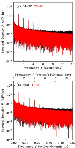
. (48) In Fig. 1a we show power spectra PH(f )for two 18-year durations of CLF horizontal-intensity hourly values: 1954.0– 1972.0 (hourly spot measurements) and 1972.0–1990.0 (1-h averages). Regular solar-quiet variation is seen as prominent diurnal peaks with frequencies of 1/d, 2/d, etc. (e.g. Olsen, 2007). Magnetic storms and disturbance are seen as a broad wash of energy across the entire range of frequencies, with a gradual “red-spectrum” decrease in energy with increasing frequency.
Important for this study are the differences in the spec-tra between the older pre-1972.0 data, when reported hourly values were spot measurements, and the newer post-1972.0 data, when reported hourly values were 1-h average-samples. The spectral power for spot measurements is higher at high frequencies than that for 1-h average-samples. Since spec-tral differences might simply be reflective of different levels of activity, these observations, on their own, are not suffi-cient to prove that different average-sample types (spot and average) suffer from different amounts of amplitude distor-tion and aliasing. But what we see in Fig. 1a is enough to motivate further investigation. We will return, at the end of Sect. 5.3, to discuss Fig. 1b.
Fig. 1.Comparison of(a)power spectral densityPH(f )as a func-tion of frequencyffor historical hourly CLF-Hdata for years when instantaneous “spot” values were reported, 1954.0–1972.0 (black), and when 1-h average-samples were reported, 1972.0–1990.0 (red); (b)synthetic spot samples (black) and 1-h average-samples (red), each constructed from 1-min CLF-H data, 1991.0–2009.0.
average-samples. In Fig. 2 we show results for a period of time recording a large magnetic storm (October 2003). As expected, we see in Fig. 2a that spot samples Hs(tj) sometimes record the extreme amplitudes of transient vari-ation, such as for the dramatic initial phase of this storm (Day 302.3) and during the storm’s second main phase (Day 303.8–304.1), while at other times transient variation is missed, such as during the hours immediately following the initial phase (Day 302.4). Magnetic-field variation at fre-quencies higher than Nyquist is not well represented by spot sampling, and because of this there is substantial aliasing, Ss(tj)Eq. (28). The signals of continuous interpolations of
the spot samples, Hs(t )Eq. (22), and the discrete aliases, Ss(t )Eq. (27), show Gibbs ringing. This tends to be corre-lated with spot samples that happen to fall on the extremes of the 1-min variation. Otherwise, before and after periods of rapid variation, ringing tends to occur in between spot val-ues. The later is a result of the fact that forts=1 h the sinc function has zero crossings at integer hours, a point we will examine again in Sect. 5.8.
In Fig. 2b we see that continuous, running averaging gives a smooth representation of the original time series, but the ex-treme amplitudes of storm-time variation are smoothed out. We have described this as amplitude distortion,A1(t )Eq. (8). Discrete sampling of the averaged time series has a contin-uous signal, H1s(t )Eq. (32), with less Gibbs ringing than that for spot sampling, and a low-frequency residual,L1s(t ) Eq. (35), that is, on average, less than aliasing of spot sam-pling.
5.3 Frequency spectra of different average-samples
Using, again, 1-min CLF-Hsource data, 1991.0–2009.0, we used formulas (42) to (46) to generate a variety of average-sample types. In Fig. 3a we see that the hourly spot sam-ples have a spectrumPsH(f )that is generally like “continu-ous variation” that is approximated by 1-min dataPH(f ). However, at high frequencies, near the Nyquist frequency (∼0.5 cycles/h), the energy of the hourly spot spectrum is higher than that for the 1-min data. This lifting of the high-frequency end of the hourly spectrum is entirely due to alias-ing, S˜s(f ) Eq. (26). In Fig. 3b we show the spectrum of aliasingPsS(f ), which can be recognized as the reflection of the 1-min spectrum through the Nyquist frequency. Because the 1-min spectrum is “red”, reflection through Nyquist re-sults in an aliasing spectrum that is “blue”, and for this rea-son, aliasing is most easily seen in Fig. 3a for frequencies immediately below Nyquist.
Fig. 2.Data from CLF recording 2 days of horizontal-intensity magnetic-field variation during the Halloween storm of October 2003: 1-min dataH (t )(red), running averagesHa(t )(black), signal of discrete samplesHas(t )(black), aliasSs(t )(brown), low-frequency residualLas(t ) (blue), and discrete samples (black dots), each for(a)instantaneous, spot samplesHs(tj)and(b)1-h average-samplesH1s(tj).
terms – those differences are due to amplitude distortion. Similar conclusions can be drawn from the spectra for Gaus-sian average-samples Fig. 3g, h.
For 2-h running averages, we see in Fig. 3e that the energy in the spectrum P2H(f ) is substantially depressed for fre-quencies near Nyquist, and, indeed, the spectrum for hourly 2-h average-samplesP2sH(f )is also substantially depressed at high frequencies. In Fig. 3f we see that aliasing spectrum P2S(f )is lower than that for 1-h Fig. 3d or Gaussian Fig. 3h average-samples, but the residual spectrumP2L(f )is higher.
Brick-wall results,PσH(f )Fig. 3i, j, are a special case; this type of average-sample has perfect frequency response below Nyquist, and therefore no low-frequency residuals at all. The lesson we can take away from these comparisons is that there is a trade-off between amplitude distortion and aliasing.
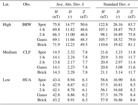
Table 2.Statistics of discrete 64-min “hourly” average-samples for 1998.0–2009.0.
Lat. Obs. Ave. Abs. Dev.δ Standard Dev.σ
H D Z H D Z
(nT) (′) (nT) (nT) (′) (nT) High BRW Spot 75.8 14.77 50.6 122.8 26.16 83.7 1-h 69.8 11.82 48.6 107.1 18.87 79.5 2-h 66.3 11.00 46.8 98.1 16.89 75.8 Gauss 69.1 11.66 48.3 105.7 18.52 79.0 Brick 71.9 12.23 49.5 110.6 19.42 81.1
Medium CLF Spot 14.5 2.32 7.8 21.6 3.23 11.8
1-h 14.1 2.24 7.8 20.9 3.10 11.7
2-h 13.8 2.17 7.7 20.4 2.97 11.4
Gauss 14.1 2.23 7.8 20.8 3.08 11.6 Brick 14.3 2.28 7.8 21.1 3.14 11.7
Low HUA Spot 43.4 8.94 6.3 58.6 16.90 8.6
1-h 42.9 8.87 6.2 57.5 16.81 8.5
2-h 42.1 8.78 6.1 56.1 16.68 8.2
Gauss 42.8 8.86 6.2 57.3 16.79 8.4 Brick 43.2 8.91 6.3 57.9 16.86 8.6
to the two periods of time shown in Fig. 1a for the histori-cal data (spot samples 1954.0–1972.0, 1-h average-samples 1972.0–1990.0). From the considerable similarity between the spectra seen in Figs. 1a, b and 3a, b, we conclude that the spectral differences in the historical CLF, seen in Fig. 1a, are almost entirely due to different averaging and sampling methods.
5.4 Statistical moments of the average-samples
As a statistical summary of magnetic-field variability recorded by the various hourly average-sample types, we cal-culate average-absolute deviations
δB= 1 NB
X
j
|B(tj)|, (49)
and standard deviations
σB= "
1 NB
X
j
|B(tj)|2 #12
, (50)
each defined here for zero-mean data; recall from Sect. 4 that we have subtracted a slowly-varying trendline. By Parseval’s theorem, the variance of the time series equals the total power integrated over all frequencies,
1 NB
X
j
|B(tj)|2= X
k
PB(fk) (51)
(Lee, 1960, p. 11; Bracewell, 1978, p. 112). Therefore, re-sults for statistical variance, Eq. (50), can be interpreted in terms of the integral of the spectral power in the frequency-domain, Eq. (48).
In Table 2 we list statistical moments for horizontal in-tensityH, declinationDand vertical intensityZ, from high (BRW), medium (CLF), and low-latitude (HUA) observa-tories. Hourly spot measurements are an unbiased repre-sentation, in a statistical sense, of the amplitude range of magnetic-field variation. It is, therefore, useful to compare the moments of spot-sample measurements with those of the other average-samples types. Without exception, brick-wall (2-h) average-samples haveδ andσ values closest to (fur-thest from) those of spot samples. Still, it is noteworthy that results for 1-h average-samples are relatively similar to those of both the Gaussian and brick-wall average-samples. 5.5 Low-frequency residual moments
Table 3.Statistics of low-frequency residualsLas(t )for 1998.0–2009.0.
Lat. Obs. Ave. Abs. Dev.δ Standard Dev.σ
H D Z H D Z
(nT) (′) (nT) (nT) (′) (nT) High BRW Spot 29.2 8.71 11.2 53.7 17.38 20.7
1-h 11.4 2.65 5.0 17.7 4.24 7.8
2-h 18.8 3.82 9.2 31.6 6.36 14.9 Gauss 11.3 2.51 5.2 17.7 3.94 8.0
Brick 0.0 0.00 0.0 0.0 0.00 0.0
Medium CLF Spot 2.1 0.39 0.4 4.2 0.75 1.0
1-h 1.0 0.17 0.2 1.6 0.28 0.4
2-h 1.8 0.31 0.6 3.0 0.50 0.9
Gauss 1.0 0.17 0.3 1.6 0.28 0.4
Brick 0.0 0.00 0.0 0.0 0.00 0.0
Low HUA Spot 4.3 0.55 0.6 8.7 1.31 0.9
1-h 1.9 0.25 0.3 3.1 0.50 0.4
2-h 3.4 0.50 0.7 5.5 0.97 0.9
Gauss 1.9 0.26 0.3 3.0 0.52 0.4
Brick 0.0 0.00 0.0 0.0 0.00 0.0
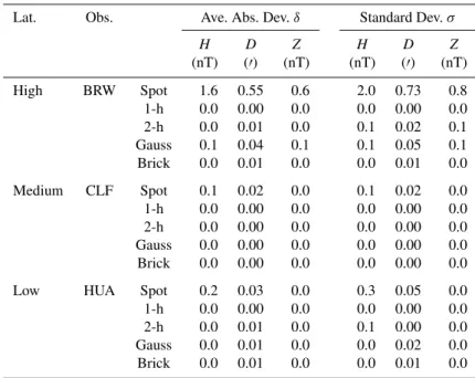
Table 4.Statistics of discrete 685×64-min “monthly” differencesǫ⋆m(tj)for 1998.0–2009.0.
Lat. Obs. Ave. Abs. Dev.δ Standard Dev.σ
H D Z H D Z
(nT) (′) (nT) (nT) (′) (nT)
High BRW Spot 1.6 0.55 0.6 2.0 0.73 0.8
1-h 0.0 0.00 0.0 0.0 0.00 0.0
2-h 0.0 0.01 0.0 0.1 0.02 0.1
Gauss 0.1 0.04 0.1 0.1 0.05 0.1
Brick 0.0 0.01 0.0 0.0 0.01 0.0
Medium CLF Spot 0.1 0.02 0.0 0.1 0.02 0.0
1-h 0.0 0.00 0.0 0.0 0.00 0.0
2-h 0.0 0.00 0.0 0.0 0.00 0.0
Gauss 0.0 0.00 0.0 0.0 0.00 0.0
Brick 0.0 0.00 0.0 0.0 0.00 0.0
Low HUA Spot 0.2 0.03 0.0 0.3 0.05 0.0
1-h 0.0 0.00 0.0 0.0 0.00 0.0
2-h 0.0 0.01 0.0 0.1 0.00 0.0
Gauss 0.0 0.01 0.0 0.0 0.02 0.0
Brick 0.0 0.01 0.0 0.0 0.01 0.0
5.6 Monthly and annual means
Monthly and annual observatory means are used for secular variation studies, and so it is useful to evaluate the effects of using different types of hourly average-samples in their con-struction. For simplicity, we define “monthly” means as the average of geomagnetic-vector components over tm=685 “hours”, each being 64 min in length,
B⋆m(tj)= 1 tm
h=+342 X
h=−342
B⋆(tj+h), (52)
with⋆denoting any chosen hourly average-sample type from Eq. (42) to Eq. (46). The difference between a monthly mean of hourly average-samples and a monthly mean of 1-min data is
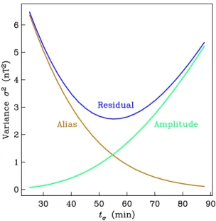
Fig. 4. Trade-off diagram, for CLF-H 1998.0–2009.0, showing variance of amplitude distortion Aσs(t ) (green), aliasing Sσs(t ) (brown), and low-frequency residualsLσs(f )(blue) for Gaussian average-samples over a range of averaging timestσ.
In Table 4 we list the statistical moments ofǫ⋆m(t ). For low and medium latitudes, average differences are less than the 1.0 nT resolution in the monthly-mean database of Chulliat and Telali (2007). As might be expected, differences are largest for spot samples from high-latitude observatories, but even these differences are small compared to the 5.0 nT stan-dard for absolute accuracy established by Intermagnet for modern 1-min data. Corresponding differences for annual means will be even smaller, by about a factor of 1/√12. The slightly larger average differences for Gaussian average-samples are mostly due to end-point differences, with the tails of each hourly Gaussian filter extending outside of each monthly boxcar averaging window. In analyzing secular variation, it is probably acceptable to use any type of hourly average-sample to construct monthly and annual means. 5.7 Optimum Gaussian filter
Our choice of a Gaussian filter withtσ=55 min minimizes the variance of the low-frequency residuals,Lσs(f )Eqs. (35) and (50). In Fig. 4 we show this quantity, along with the vari-ance of amplitude distortionAσs(t )and aliasing Sσs(t ), as function oftσ. Amplitude distortion (aliasing) increases (de-creases) with increasingtσ, but there is an inflection point at tσ=55 min where the residuals are minimized. This method of selecting an optimal averaging width is a simple example of what is sometimes called “filter design”.
It is tempting to try to relate the optimized Gaussian fil-ter to a boxcar average of a certain averaging width. While we hesitate to read too much into such comparisons, we have already observed from Table 3 that some of the properties
of 1-h average-samples are similar to those of the optimum Gaussian filter. The small statistical differences between these two average-sample types are probably not very signif-icant for most uses of observatory hourly values. Of course, the redeeming quality of 1-h average-samples is that they are easy to calculate, even easier than Gaussian average-samples. 5.8 Autocorrelation and avoiding the Gibbs effect While it is a standard practice to use power spectra to check for periodic signals and to display Fourier amplitudes in the frequency domain, in the time domain the corresponding quantity is autocorrelation. For a real function, such as an observatory magnetic-field time series, autocorrelation is de-fined by the integral
CB(τ )= lim 8→∞
1 8
Z +8/2
−8/2
B(φ)B(φ+τ )dφ, (54) (Press et al., 1992, “correl”), where τ represents a relative time lag. By the Wiener-Khinchine or “auto-correlation” the-orem (Lee, 1960, p. 11; Bracewell, 1978, p. 115), an autocor-relation is related to a power spectrum by Fourier transforma-tion,
FnCB(τ )o=PB(f ). (55) Despite this duality, some properties of a time series are more easily seen in power spectra, while others are more easily seen in autocorrelation.
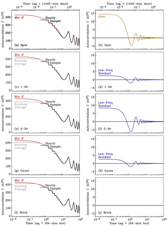
In Fig. 5 we show autocorrelations for the source 1-min dataCH(τ ), continuous running averagesCaH(τ ), and average-samplesCasH(τ )for CLF-H 1991.0–2009.0. Promi-nent solar-quiet diurnal peaks are seen with time lags of 1d, 2d, etc.; these correspond to the diurnal peaks in fre-quency of 1/d seen in the power spectra of Fig. 3. For very short time lags, less than the averaging duration, autocorrela-tionsCaH(τ ) are flat. These results are all to be expected. What is perhaps more interesting are the autocorrelations for low-frequency residuals,CLa(τ )Eq. (35). For spot sam-pling, residuals are entirely due to aliasing, and since alias-ing residuals tend to be larger than those for other average-sample types, the autocorrelation of spot-sampling residuals has a larger zero-time-lag base value. For all average-sample types, other than the brick-wall, there is significant Gibbs-effect ringing out to time lags of several hours. Close inspec-tion of Fig. 5 shows that the zero crossings ofCaL(τ )occur, very nearly, at integer hours (64-min hours). This is consis-tent with the observation we made in Sect. 5.2 that hourly average-samples avoid most Gibbs ringing by straddling the zero crossings of the sinc function.
Fig. 6. Scatter plots of discrete 1-hH1s(tj)versus brick-wall average-samplesHbs(tj)for(a)high latitude (BRW),(b)medium latitude (CLF), and(c)low latitude (HUA). Also given, for each case, are correlation coefficientsρand proportionalitiesα(shown as a fitted line). Data used are for 1998.0-2009.0, and densities are for 100.0, 10.0, 1.0, and 0.1% of the data.
Fig. 7.Scatter plots of discrete 1-h average-samplesH1s(tj)versus spot samplesHs(tj)for(a)high latitude (BRW),(b)medium latitude (CLF), and(c)low latitude (HUA). Also given, for each case, are correlation coefficientsρand proportionalitiesα(shown as a fitted line). Data used are for 1998.0–2009.0, and densities are for 100.0, 10.0, 1.0, and 0.1% of the data.
types have some combination of amplitude distortion and aliasing. It is useful, therefore, to compare linear correlations ρbetween brick-wall and other average-sample types, ρ= 1
NB X
j
Bas(tj)Bbs(tj)
σB asσbsB
, (56)
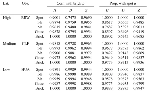
(Press et al., 1992, “pearsn”), defined here for zero-mean data; recall from Sect. 4 that we have subtracted a slowly-varying trendline. A correlation close to unity means that the relative amplitude, phase, and frequency of continuous magnetic-field variation below Nyquist are being accurately recorded. In Fig. 6 we show scatter plots for brick-wall and 1-h average-samples. In Table 5 we list correlations for each magnetic-field component and for each observatory. In gen-eral, spot and 2-h average-samples have the lowest
correla-tions with brick-wall average-samples, while 1-h and Gaus-sian average-samples are very highly correlated with brick-wall average-samples.
Since spot measurements are a statistically unbiased sam-pling of the amplitude range of magnetic-field variation, it is useful to compare their proportionalitesαwith the other average-samples,
Table 5.Correlations with brick-wall average samples and proportionalities with spot samples, 1998.0–2009.0.
Lat. Obs. Corr. with brickρ Prop. with spotα
H D Z H D Z
High BRW Spot 0.9001 0.7475 0.9690 1.0000 1.0000 1.0000 1-h 0.9874 0.9759 0.9955 0.8617 0.6565 0.9485 2-h 0.9615 0.9480 0.9841 0.7687 0.5393 0.9013 Gauss 0.9878 0.9795 0.9954 0.8597 0.6496 0.9419 Brick 1.0000 1.0000 1.0000 0.8902 0.6745 0.9685 Medium CLF Spot 0.9818 0.9728 0.9963 1.0000 1.0000 1.0000 1-h 0.9973 0.9962 0.9994 0.9677 0.9573 0.9862 2-h 0.9906 0.9881 0.9972 0.9427 0.9142 0.9669 Gauss 0.9973 0.9962 0.9994 0.9649 0.9514 0.9837 Brick 1.0000 1.0000 1.0000 0.9773 0.9713 0.9936 Low HUA Spot 0.9891 0.9989 0.9944 1.0000 1.0000 1.0000 1-h 0.9986 0.9998 0.9989 0.9808 0.9946 0.9837 2-h 0.9959 0.9994 0.9948 0.9578 0.9873 0.9563 Gauss 0.9987 0.9998 0.9988 0.9775 0.9935 0.9799 Brick 1.0000 1.0000 1.0000 0.9888 0.9975 0.9947
Fig. 8. Comparison of power spectral densityPH(f )as a func-tion of frequencyffor historical hourly ESK-Hdata obtained from WDC-CE, 1917.0–1932.0 (black) and 1932.0–1947.0 (red).
magnetic-field component and for each observatory. With-out exception, brick-wall (2-h) average-samples are the most (least) directly proportional to spot samples. Results for 1-h average-samples are relatively similar to those of both Gaus-sian and brick-wall average-samples.
5.10 ESK hourly values at the WDCs
In Sect. 2 we mentioned that the pre-1932.0 hourly WDC-CE ESK data are 2-h average-samples, with each datum formed by averaging two adjacent 1-h average-samples from
the original observatory yearbooks. In Fig. 8 we show frequency-domain power spectra of historical ESK-H data obtained from WDC-CE, separately for the years 1917.0– 1932.0 and 1932.0–1947.0. As a result of 2-h averaging, the frequency content of the data for 1917.0–1932.0 has been dramatically altered. Since many researchers assume that data obtained from a WDC are those that the observatories originally reported, it would be desirable to return the WDC-CE holdings of the ESK data to their original form, possibly by using the digital data held at Kyoto. Otherwise, it would be useful for the data to be flagged as having been changed.
Note added after journal review: we are happy to have learned that the pre-1932.0 hourly WDC-CE ESK data have been restored to their original yearbook values (S. Macmil-lan, personal communication, 2010).
6 Conclusions
Nyquist, 1-h average-samples from medium and low-latitude observatories are only slightly contaminated by amplitude distortion and aliasing – their average low-frequency resid-uals are less than the 5.0 nT absolute accuracy level estab-lished by Intermagnet as a modern operational standard for observatories. High-latitude 1-h average-samples have more amplitude distortion and aliasing, but the natural magnetic “signal” is also larger at high latitudes. 1-h average-samples constructed using an optimal Gaussian filter are not signifi-cantly more accurate than simple 1-h average values. There-fore, we recommend the continuation of the standard practice by observatories and World Data Centers for reporting sim-ple 1-h-average hourly values. Of course, this does not pre-clude the production of other data-based products, including other types of hourly values, but maintaining continuity with the historical 1-h-average time series should be recognized as an important priority.
Acknowledgements. The results presented here rely on data col-lected at the Barrow, Chambon la Forˆet, Eskdalemuir, and Huan-cayo observatories. The Barrow observatory is operated by the USGS Geomagnetism Program. We thank the Institut de Physique du Globe de Paris (France), the British Geological Survey (Great Britain), and the Instituto Geofisico (Per´u) for continuing to support the operation of their observatories. We acknowledge Intermagnet (www.intermagnet.org) for facilitating the dissemination of mag-netic observatory data and for promoting high standards of magmag-netic observatory practice. We thank the Edinburgh and Kyoto World Data Centers for archiving observatory data and making them read-ily available to the scientific community. We thank the Boulder World Data Center (NGDC) for use of their observatory yearbooks. We thank P. S. Earle, J. W. Kirchner, K. Mursula, and L. Sval-gaard for useful conversation/communication. We thank A. Chul-liat, C. A. Finn, V. Lesur, and S. Macmillan, for reviewing a draft manuscript.
Topical Editor I. A. Daglis thanks S. Macmillan, A. Chulliat, and another anonymous referee for their help in evaluating this paper.
References
Barraclough, D. R., Clark, T. D. G., Cowley, S. W. H., Hibberd, F. H., Hide, R., Kerridge, D. J., Lowes, F. J., Malin, S. R. C., Murphy, T., Rishbeth, H., Runcorn, S. K., Soffel, H. C., Stew-art, D. N., StuStew-art, W. F., Whaler, K. A., and Winch, D. E.: 150 years of magnetic observatories: Recent researches on world data, Surv. Geophys., 13, 47–88, 1992.
Bendat, J. S. and Piersol, A. G.: Random Data: Analysis and Mea-surement Procedures, John Wiley & Sons, New York, NY, 2000. Bloxham, J. and Jackson, A.: Simultaneous stochastic inversion for geomagnetic main field and secular variation 2. 1820–1980, J. Geophys. Res., 94, 15753–15769, 1989.
Bracewell, R. N.: The Fourier Transform and its Applications, McGraw-Hill Book Company, New York, NY, 1978.
Brooke, C.: On the automatic registration of magnetometers, and other meteorological instruments, by photography, Phil. Trans. R. Soc. Lond., 137, 69–77, 1847.
Campbell, W. H.: The regular geomagnetic-field variations during quiet solar conditions, in: Geomagnetism, Volume 3, edited by: Jacobs, J. A., pp. 385–460, Academic Press, London, UK, 1989. Chapman, S. and Bartels, J.: Geomagnetism, Volumes 1 & 2,
Ox-ford Univ. Press, London, UK, 1962.
Chulliat, A. and Telali, K.: World monthly means database project, in: Proceedings of the XIIth IAGA Workshop on Geomagnetic Instruments, Data Acquisition, and Processing, edited by: Reda, J., pp. 268–274, Publs. Inst. Geophys. Pol. Acad. Sc., 2007. Conte, S. D. and de Boor, C.: Elementary Numerical Analysis,
McGraw-Hill Book Company, New York, NY, 1980.
Courtillot, V. and Le Mou¨el, J. L.: Time variations of the Earth’s magnetic field: From daily to secular, Ann. Rev. Earth Planet. Sci., 16, 389–476, 1988.
Egbert, G. D., Booker, J. R., and Schultz, A.: Very long period mag-netotellurics at Tucson Observatory: Estimation of impedances, J. Geophys. Res., 97, 15113–15128, 1992.
Fouassier, D. and Chulliat, A.: Extending backwards to 1883 the French magnetic hourly data series, in: Proceedings of the XII-Ith IAGA Workshop on Geomagnetic Instruments, Data Acqui-sition, and Processing, edited by: Love, J. J., pp. 86–94, US Ge-ological Survey, 2009.
Hazard, D. L.: Results of Observations Made at the United States Coast and Geodetic Survey Magnetic Observatory at Chel-tenham, Maryland, 1915 and 1916, Govt. Printing Office, Wash-ington, D.C., 1918.
Jankowski, J. and Sucksdorff, C.: Guide for Magnetic Measure-ments and Observatory Practice, IAGA, Warsaw, Poland, 1996. Kanasewich, E. R.: Time Sequence Analysis in Geophysics, Univ.
Alberta Press, Alberta, Canada, 1981.
Karinen, A. and Mursula, K.: A new reconstruction of the Dst index for 1932–2002, Ann. Geophys., 23, 475–485, doi:10.5194/angeo-23-475-2005, 2005.
Kerridge, D. J.: INTERMAGNET: Worldwide near-real-time geomagnetic observatory data, Proc. ESA Space Weather Workshop, ESTEC, Noordwijk, The Netherlands, http://www. esa-spaceweather.net/spweather/workshops/workshops.html, 2001.
Kirchner, J. W.: Aliasing in 1/fα noise spectra: Origins, conse-quences, and remedies, Phys. Rev., E 71, 066 110, 2005. Lee, Y. W.: Statistical Theory of Communication, John Wiley &
Sons, New York, NY, 1960.
Love, J. J.: Magnetic monitoring of Earth and space, Physics Today, 61, 31–37, 2008.
Love, J. J.: Missing data and the accuracy of magnetic-observatory hour means, Ann. Geophys., 27, 3601–3610, doi:10.5194/angeo-27-3601-2009, 2009.
Macmillan, S. and Droujinina, A.: Long-term trends in geomag-netic daily activity, Earth Planets Space, 59, 391–395, 2007. Marsal, S. and Curto, J. J.: A new approach to the hourly mean
com-putation problem when dealing with missing data, Earth Planets Space, 61, 945–956, 2009.
Martini, D. and Mursula, K.: Correcting the geomagnetic IHV in-dex of the Eskdalemuir observatory, Ann. Geophys., 24, 3411– 3419, doi:10.5194/angeo-24-3411-2006, 2006.
Meteorological Office: The Observatories’ Year Book 1931, His Majesty’s Stationary Office, London, UK, 1933.
Meteorological Office: The Observatories’ Year Book 1932, His Majesty’s Stationary Office, London, UK, 1934.
Olsen, N.: Natural sources for electromagnetic induction studies, in: Encyclopedia of Geomagnetism and Paleomagnetism, edited by: Gubbins, D. and Herrero-Bervera, E., pp. 743–746, Springer-Verlag, New York, NY, 2007.
Parkinson, W. D.: Introduction to Geomagnetism, Scottish Aca-demic Press, Edinburgh, UK, 1983.
Press, W. H., Teukolsky, S. A., Vetterling, W. T., and Flannery, B. P.: Numerical Recipes, Cambridge Univ. Press, Cambridge, UK, 1992.
Pr¨olss, G. W.: Physics of the Earth’s Space Environment, Springer-Verlag, Berlin, Germany, 2004.
Rasson, J. L.: INTERMAGNET, in: Encyclopedia of Geo-magnetism and PaleoGeo-magnetism, edited by: Gubbins, D. and Herrero-Bervera, E., pp. 715–717, Springer-Verlag, New York, NY, 2007.
Sabaka, T. J., Olsen, N., and Purucker, M. E.: Extending comprehensive models of the Earth’s magnetic field with Ørsted and CHAMP data, Geophys. J. Int., 159, 521–547, doi:10.111/j.1365-246X.2004.02421.x, 2004.
Schmidt, A.: Ergebnisse der magnetischen Beobachtungen In Pots-dam im Jahre 1905, vol. 196, Ver¨off. K. Preuss. Meteor. Inst., Berlin, 1908.