A comparative study of the response of modeled non-drizzling stratocumulus to meteorological and aerosol perturbations

(1)

www.atmos-chem-phys.net/13/2507/2013/ doi:10.5194/acp-13-2507-2013

Atmospheric

Chemistry

and Physics

Geoscientiic

A comparative study of the response of modeled non-drizzling

stratocumulus to meteorological and aerosol perturbations

J. L. Petters1, H. Jiang2, G. Feingold3, D. L. Rossiter1, D. Khelif4, L. C. Sloan1, and P. Y. Chuang1 1_{Earth and Planetary Sciences Department, University of California – Santa Cruz, Santa Cruz, CA, USA} 2_{Cooperative Institute for Research in the Atmosphere, Fort Collins, CO, USA}

3_{NOAA/Earth System Research Laboratory, Boulder, CO, USA}

4_{Department of Mechanical and Aerospace Engineering, University of California – Irvine, Irvine, CA, USA}

Correspondence to:J. L. Petters (jlpetter@ucsc.edu)

Received: 4 September 2012 – Published in Atmos. Chem. Phys. Discuss.: 16 October 2012 Revised: 14 February 2013 – Accepted: 22 February 2013 – Published: 5 March 2013

Abstract. The impact of changes in aerosol and cloud droplet concentration (Na andNd) on the radiative forcing

of stratocumulus-topped boundary layers (STBLs) has been widely studied. How these impacts compare to those due to variations in meteorological context has not been investi-gated in a systematic fashion for non-drizzling overcast stra-tocumulus. In this study we examine the impact of observed variations in meteorological context and aerosol state on day-time, non-drizzling overcast stratiform evolution, and deter-mine how resulting changes in cloud properties compare.

Using large-eddy simulation (LES) we create a model base case of daytime southeast Pacific coastal stratocumu-lus, spanning a portion of the diurnal cycle (early morning to near noon) and constrained by observations taken dur-ing the VOCALS (VAMOS Ocean-Atmosphere-Land Study) field campaign. We perturb aerosol and meteorological prop-erties around this base case to investigate the stratocumu-lus response. We determine perturbations in the cloud top jumps in potential temperatureθand total water mixing ratio

qt from ECMWF Re-analysis Interim data, and use a set of Ndvalues spanning the observable range. To determine the

cloud response to these meteorological and aerosol perturba-tions, we compute changes in liquid water path (LWP), bulk optical depth (τ) and cloud radiative forcing (CRF).

We find that realistic variations in the thermodynamic jump properties can elicit a response in the cloud proper-ties of τ and shortwave (SW) CRF that are on the same order of magnitude as the response found due to realistic changes in aerosol state (i.eNd). In response to increases in Nd, the cloud layer in the base case thinned due to increases

in evaporative cooling and entrainment rate. This cloud thin-ning somewhat mitigates the increase inτ resulting from in-creases inNd. On the other hand, variations inθandqtjumps

did not substantially modifyNd. The cloud layer thickens in

response to an increase in theθjump and thins in response to an increase in theqtjump, both resulting in aτ and SW

CRF response comparable to those found from perturbations inNd. Longwave CRF was not substantially altered by the

perturbations we tested.

We find that realistic variations in meteorological context can elicit a response in CRF andτ on the same order of mag-nitude as, and at times larger than, that response found due to realistic changes in aerosol state. We estimate the limits on variability of cloud top jump properties required for accurate observation of aerosol SW radiative impacts on stratocumu-lus, and find strict constraints: less than 1 K and 1 g kg−1in the early morning hours, and order 0.1 K and 0.1 g kg−1close to solar noon. These constraints suggest that accurately ob-serving aerosol radiative impacts in stratocumulus may be challenging as co-variation of meteorological properties may obfuscate aerosol-cloud interactions.

1 Introduction

(2)

climate projections (Randall et al., 2007). The difficulty in representing stratiform clouds in large-scale models is exac-erbated by their sensitivity to changes in aerosol state and in the “meteorological context” in which the cloud system resides.

The impacts of perturbations in aerosol state on the radia-tive properties of stratiform cloud systems have been widely studied. These studies have focused on changes in cloud optical properties (e.g. Twomey and Wojciechowski, 1969; Twomey, 1977; Coakley et al., 1987) and changes in cloud system evolution (e.g. Albrecht, 1989). The impact of aerosol on stratiform cloud has been of particular interest and has been extensively studied with models (e.g. Jiang et al., 2002; Ackerman et al., 2004; Lu and Seinfeld, 2005; Wood, 2007; Bretherton et al., 2007; Sandu et al., 2008; Hill et al., 2008; Petters et al., 2012), remote sensing (e.g. Nakajima et al., 1991; Han et al., 1998; Sekiguchi et al., 2003; Kaufman et al., 2005; Quaas et al., 2006; Painemal and Zuidema, 2010) and in-situ observations (e.g. Brenguier et al., 2000; Durkee et al., 2000; Twohy et al., 2005; Ghate et al., 2007; Lu et al., 2007). Other recent studies have focused more attention on the the impact that meteorological context can have on aerosol-cloud interactions (Matsui et al., 2006; George and Wood, 2010; Painemal and Zuidema, 2010; Wang et al., 2010; Mechem et al., 2012).

We define “meteorological context” as those large-scale features of the atmosphere and surface that influence the stratiform cloud system on the time scale of interest (which in this study is less than 1 day) that are not strongly influenced by cloud evolution. For example, solar insolation, large-scale subsidence rate and the boundary layer jump properties would be considered part of this meteorological context. In contrast, the temperature and humidity of the boundary layer are not part of this context because they can respond rapidly to changes in the cloud.

Variations in this meteorological context can substan-tially influence the evolution of stratiform cloud systems. For example, changes in the potential temperature (θ) jump strength can influence entrainment mixing (Lilly, 1968; Sul-livan et al., 1998), while changes in free tropospheric mois-ture content (free troposphericqt) can lead to changes in the

amount of evaporative cooling due to entrainment (Acker-man et al., 2004). The meteorological context also can influ-ence the radiative forcing of these cloud systems. Increasing aerosol concentrationNacan lead to reductions in liquid

wa-ter path (LWP) when low relative humidity air resides above the boundary layer (Ackerman et al., 2004). The thermody-namic structure of the sub-cloud layer can influence the frac-tion of drizzle reaching the surface, which in turn can influ-ence boundary layer dynamics and cloud evolution (Feingold et al., 1996; Ackerman et al., 2009).

Furthermore, these variations can also potentially obfus-cate the impact of aerosol on cloud evolution. The results of Matsui et al. (2006) suggest aerosol perturbations on cloud radiative forcing of stratiform cloud systems could not be

studied in isolation; thermodynamics and the diurnal cycle also should be taken into account. Using satellite and reanal-ysis data, George and Wood (2010) found that variability in cloud microphysics contributed to less than 10 % of the vari-ability in observed albedo in a stratocumulus-dominated re-gion. Variability in albedo was mostly related to variability in LWP and cloud fraction. Additionally, because meteoro-logical and aerosol states are dependent on air-mass history, the two states tend to correlate in observations (Stevens and Feingold, 2009). For example, during the 2nd Aerosol Char-acterization Experiment (ACE-2, Brenguier et al., 2003) it was found that low aerosol concentrations were correlated with cool, moist maritime air masses while high aerosol con-centrations were correlated with warm, dry continental air masses.

For these many reasons it can be difficult to disentangle the changes in the aerosol state and meteorological context in order to isolate the aerosol forcing (Stevens and Feingold, 2009). In observational studies, it is typically assumed that the meteorological context is approximately constant during the observational period so changes in cloud evolution are primarily determined by changes in aerosol. How constant the meteorological context must be for this assumption to be valid remains an open question. In modeling studies of aerosol-cloud interactions in stratiform cloud systems, the initial meteorological context can be set constant, thereby re-moving its potential to influence cloud evolution. Analyses of the sensitivity to meteorological context exist in some mod-eling studies (e.g. Jiang et al., 2002; Sandu et al., 2008), and in this study we expand upon such analyses.

In this study we examine how stratiform cloud systems are affected by variability in meteorological context and aerosol state and evaluate their comparative importance. Specifically, we address the following questions:

Q1 Given observed variations in meteorological context

1mand aerosol state1a, how do the resulting changes in stratiform cloud properties1ccompare?

Q2 What physical processes and interactions lead to these changes in cloud?

We use a numerical modeling framework for this study because we can independently vary meteorological context and aerosol state. Using large-eddy simulation (LES), we investigate stratiform cloud evolution and the response of this evolution to variations in meteorological and aerosol changes. We determine realistic variations in meteorological context1m through use of European Centre for Medium-Range Weather Forecasting (ECMWF) Re-analysis Interim (ERA-Interim) data (Uppala et al., 2005, 2008).

For objective comparison of the cloud evolution to vari-ations in meteorological context1mand aerosol state1a, we compute the response of the cloud properties (1c) of

(3)

Table 1.Model base case configuration and settings for Regional Atmospheric Modeling System (RAMS) in large-eddy simulation. Where applicable, configuration values are based on in-situ observations from the Twin Otter.

Model Part Setting Notes/Reference

grid resolution 50 m horizontal, 10 m vertical refined to 5 m near boundary layer top

vertical resolution consistent with Stevens et al. (2005)

domain size 3.4 km on a side, 2 km in vertical simulates one full convective cell (Caldwell and Bretherton, 2009)

boundaries cyclic lateral boundary conditions, rigid bottom and top

Rayleigh friction layer in top 16 vertical layers for removal of spurious gravity wave reflection

model timestep 0.5 s for model spin-up, 1 s thereafter meets CFL criterion

microphysics parameterization: bin microphysical model (Tzivion et al., 1987; Feingold et al., 1988; Tzivion et al., 1989), described in Feingold et al. (1996); Stevens et al. (1996)

25 bins for non-drizzling case mass-doubling between bins

radiation parameterization: two-stream solver (Harrington, 1997)

correlated-k distribution spectral band model 15 shortwave and 12 longwave spectral inter-vals (Cole, 2005)

binned cloud optical properties (Harrington and Olsson, 2001)

thermodynamic profile above domain Iquique, Chile sounding from 12:00 Z, 19 Oc-tober 2008

radiative timestep 5 s meets strict criterion of Xu and Randall (1995)

sub-grid scale parameterization Deardorff isotropic diffusion scheme (Deardorff, 1980)

subsidence 5×10−6·z m s−1 z is height; expression follows Ackerman et al.

(2009), coefficient chosen for best match to ob-servations of boundary-layer height

sea surface temperature constant 289.7 K as measured from Twin Otter for non-drizzling

case, used for radiative computation only surface fluxes constant 3 and 27 W m−2 for sensible/latent

fluxes

as measured from Twin Otter

cloud radiative forcing (CRF) to variations in meteorologi-cal context and aerosol state and see how this response com-pares to the other two. Many modeling studies of aerosol-cloud interactions on stratocumulus simulate nighttime aerosol-cloud evolution (e.g. Bretherton et al., 2007; Hill et al., 2008) and as such rely on modeled response in τ to determine the importance of aerosol’s influence on CRF. To serve as the model base case for this comparative study, we first create a observationally-constrained LES of non-drizzling overcast stratocumulus based on in-situ observations taken from the CIRPAS (Center for Interdisciplinary Remotely-Piloted Aircraft Studies) Twin Otter during the VOCALS (VAMOS Ocean-Atmosphere-Land Study) field campaign (Wood et al., 2011). Describing the LES model description and configuration, the observations used to create the model base case, and the comparison between LES output and ob-servations (Sects. 2 to 4) comprise the first part of this study. In the second part we detail the comparative study, includ-ing the experimental design, model output and computed re-sponses (Sects. 5 to 7).

We find that realistic variations in meteorological context can elicit a response in CRF andτ on the same order of mag-nitude as, and at times larger than, those responses found due to realistic changes in aerosol state. Our results suggest that

careful consideration of consistency in meteorological con-text (the jump properties in particular) must be given when planning observational studies of aerosol-cloud interactions and their impact on stratocumulus radiative properties.

2 Model description

Large-eddy simulation (LES) is a commonly used numerical technique for studying cloud-topped boundary layers. Be-cause it is capable of resolving turbulent motions and the interactions among microphysics, radiation, and dynamics (Stevens et al., 2005; Ackerman et al., 2009; Stevens and Feingold, 2009), it is the most applicable numerical tool for our study. Other cloud-scale numerical modeling techniques (e.g. Harrington et al., 2000; Pinsky et al., 2008) require dy-namical motions as inputs. Hence the meteorological context cannot be varied within these models, and interactions be-tween dynamics and either radiation or microphysics cannot be represented.

(4)

RAMS are specified in Table 1. Wang et al. (2010) and Mechem et al. (2012) used LES in their respective studies of aerosol and meteorological forcings in stratocumulus. How-ever, they focused their studies on the mesoscale organiza-tion of stratocumulus (i.e. open and closed cells), simulating larger regions with both coarser spatial resolution and longer timescales than we do in this study.

We use a bin microphysical model (Feingold et al., 1996; Stevens et al., 1996) in order to best reproduce observed drop size distributions. This particular microphysical model has been previously used for several studies of aerosol-cloud in-teractions within the boundary layer (e.g. Jiang et al., 2002; Xue and Feingold, 2006; Hill et al., 2009). In this model aerosol is assumed to be fully-soluble ammonium sulfate with a lognormal size distribution that is constant over time and space (Xue and Feingold, 2006). For the base case the mean aerosol diameter Dp is 0.12 µm. We use a

to-tal aerosol concentration Na=450 cm−3, giving an initial

average cloud droplet concentration valueNd=425 cm−3,

matching the mean value from aircraft observations on the VOCALS case study that we are simulating (see next sec-tion).

In this study we simulate only overcast, or nearly overcast, stratocumulus. There are a few reasons for this constraint. First, our large-eddy simulations assume homogenous mix-ing within model grid-boxes. While Hill et al. (2009) did not find this assumption to substantially influence the LWP and cloud optical depth of a modeled overcast stratocumulus layer, it may be expected to be more impactful in simula-tion of a thin, broken stratocumulus layer. Second, the radi-ation parameterizradi-ation we use (Harrington, 1997) employs the Independent Column Approximation (ICA), in which ra-diation is not exchanged between model columns. Use of the ICA could lead to biases in both computations of cloud radia-tive heating and cloud radiaradia-tive forcing (e.g. Zuidema et al., 2008), especially at model resolutions used in our study (Ca-halan et al., 2005). Finally, large-eddy simulations coupled with a bin microphysical model are computationally inten-sive, and simulating more than a a fraction of the stratocumu-lus diurnal cycle is impractical. For these reasons our simula-tions end when our observationally-constrained model cloud layer begins to break up (i.e. cloud fraction becomes less than unity).

Schubert et al. (1979) determined two separate response timescales for the STBL; one of thermodynamic adjustment (changes in water vapor mixing ratio qv and cloud base,

for example) on a timescale of less than a day, and one for the inversion height, adjusting on timescales of 2 to 5 days. Bretherton et al. (2010) showed that STBLs simulated with LES or mixed-layer models evolve to equilibrium states (thin, broken cloud or thick, overcast cloud) over the course of several days, and these equilibria are dependent on the ini-tial inversion height. The findings of Bretherton et al. (2010) suggest that the cloud response to perturbations in meteorol-ogy and aerosol might be less important on longer timescales

than those investigated here because changes in inversion height, driven by changes in large-scale subsidence, might play the primary role. Thus our results are most applicable to the shorter thermodynamic adjustment timescale. We sim-ulate stratocumulus evolution during daytime hours, corre-sponding to the time of the observations and during which changes in cloud properties are most relevant to shortwave (SW) radiative forcing.

While LES is the most appropriate tool for this study, like any model, it has imperfections and limitations. One issue common to LES of the stratocumulus-topped boundary layer (STBL) is their propensity to over-entrain air across the cloud top interface (Stevens et al., 2005; Caldwell and Bretherton, 2009). Sub-grid scale parameterizations commonly used in LES simplify many small-scale processes important in STBL entrainment (e.g. Mellado, 2010), and one consequence of this simplification is over-entrainment. Below we describe measures to lessen the impact of this over-entrainment on our modeling output.

3 Observations

To build a realistic, observationally-based large-eddy sim-ulation of stratocumulus, i.e. the model base case, we use in-situ observations taken from the CIRPAS Twin Otter dur-ing the VOCALS (VAMOS Ocean-Atmosphere-Land Study) field campaign. We focus on a simpler non-drizzling case be-cause the existence of drizzle increases the complexity of the evolution of microphysics and dynamics in the STBL (Lu et al., 2007; Ackerman et al., 2009). During VOCALS, driz-zle in the coastal stratocumulus observed from the Twin Otter was negligible (≪0.1 mm day−1).

Table 2 briefly describes the relevant instrumentation on board and parameters observed by the Twin Otter during VO-CALS. Of particular note is the Phase-Doppler Interferom-eter (PDI), which provides detailed microphysical informa-tion about the cloud layer (Chuang et al., 2008). The PDI measures the drop size distribution for a size range from 2.0 to 150 µm in 128 bins. Phase-Doppler Interferometer inte-grated liquid water content (LWC) has been previously com-pared with LWC as measured from the Gerber PVM-100 (Chuang et al., 2008). Because of the relatively low effi-ciency with which the PVM-100 samples droplets larger than

∼30 to 40 µm (Wendisch et al., 2002), we use the PDI-derived LWC in our study. Sampling of the cloud droplet distribution with the PDI also covers a broader size range more appropriate for comparisons with the LES. Because of the low drizzle rates, the contribution to LWC by drops larger than 100 µm is negligible.

(5)

Table 2.Aerosol and cloud instrument payload on Twin Otter during field campaigns. Abbreviated list; only instruments referenced in this article are listed.

Parameter Instrument Measured at Range Detected/Error

Liquid Water Content Gerber PVM-100 10 Hz <40 µm (nominal)

Cloud Droplet Size Distribution Phase Doppler Interferometer (PDI) 1 to 10 Hz 2–100µm

Drizzle Size Distribution Cloud Imaging Probe (CIP) 1 Hz 100–2000µm

Accumulation-mode Aerosol Size Distribution Passive Cavity Aerosol Spectrometer (PCASP) 1 Hz 0.1–2.6µm Particle Number Concentration TSI Condensation Particle Counter (CPC) 3010 10 Hz diameter>10 nm

Turbulent velocities Nose-mounted gust probe 100 Hz ±0.1 m s−1

Ambient Temperature Rosemount 10 Hz −50 to 50,±0.1◦C

Dew Point Temperature EdgeTech chilled mirror 1 Hz −50 to 50,±0.2◦C

Water Vapor Content Li-Cor 20 Hz 0 to 42±0.005 g m−3

Sea Surface Temperature Heitronics KT 19.85 Pyrometer 10 Hz −5 to 45◦C

Barometric Pressure Setra barometric transducers 100 Hz 600–1100±75 mb

Table 3.Thermodynamic profile (sounding) used to initialize model. Where applicable, original values from observations (before modifi-cation for use in this study) are shown in parentheses. The surface pressure was initialized at 1018.0 mb. Temperature and moisture values above the inversion were those observed immediately before the flight legs.

Layer Potential Total Water U wind V wind

Temperature (K) Content (g kg−1) (m s−1) (m s−1)

0–980 m (0–1040 m) 287.30 7.55 (7.35) −0.50 0.70

990 m (1050 m ) 293.65 4.17 (4.07) 0.55 −0.50

1000 m (1060 m) 300.00 0.80 1.60 −1.70

above 1000 m (1050 m) observed observed 1.60 −1.70

observations are averaged to 1 Hz (for a horizontal resolu-tion of 55 m) over five∼30 km flight legs: two below-cloud (both near the surface), one just below cloud base, and two in-cloud (mid-cloud and cloud top). During this day a STBL with cloud of∼300 m thickness was observed, and the LWC increased nearly adiabatically with height. We compared the atmospheric profiles taken before and after the flight legs and found little change in the thermodynamic and wind pro-files. Averaged over the depth of the boundary layer, the profiles exhibited the following changes during the obser-vational period: 0.2 K decrease inθ, 0.16 g kg−1increase in

qv, 1.0 m s−1increase in easterly wind speed, and 0.7 m s−1

increase in northernly wind speed. The inversion height re-mained fairly constant over the observational period, indi-cating that net entrainment or detrainment in the boundary layer was negligible. Vertical profiles of vertical velocity and equivalent potential temperature show that the observed STBL is well-mixed. Taken together, these STBL properties provide us with a “canonical” stratocumulus case to model with LES; that is, a case that has similar characteristics to those previously studied with LES (e.g. Dyunkerke et al., 2004; Stevens et al., 2005).

Potential temperature and moisture content jumps at the cloud top interface were +12.7 K and −6.55 g kg−1, re-spectively. The Passive Cavity Aerosol Spectrometer Probe (PCASP) showed sub-cloud accumulation mode aerosol con-centrations elevated from those expected for clean maritime

conditions (∼600 cm−3), at least partially accounting for the low drizzle rates. Observed average sea surface temperature and surface flux values are shown in Table 1.

4 Comparing model performance to observations

The sounding data used to initialize the model are described in Table 3. We initialized the base simulation at 07:30 UTC, five hours prior to the hour of the five∼30 km flight legs, giving the LES ample time to spin-up realistic boundary layer eddies. Because of this time difference, we found it necessary to modify the sounding data from that taken by the Twin Ot-ter so that the simulated boundary layer would reasonably compare to that observed. These modifications, also shown in Table 3, were (a) increasing qt content in the boundary

layer by 0.2 g kg−1(a 3 % increase over the measured value, and (b) lowering the height of the inversion by 60 m (from 1040 m to 980 m).

Furthermore, we require thermodynamic profile data from the top of the model domain (2 km) to the top of the atmo-sphere (TOA) for accurate radiative computations. We use the 12Z sounding from Iquique, Chile on the same day as the flight observations were taken. Using the Iquique sound-ing ensured that free tropospheric qt values in the

(6)

2850 290 295 300 305 200

400 600 800 1000 1200

Potential temperature (K)

Height (m)

NODIFF DIFF OBS

0 1 2 3 4 5 6 7 8

0 200 400 600 800 1000 1200

Water vapor mixing ratio (g kg−1)

Height (m)

NODIFF DIFF OBS

(a) (b)

OBSERVED CLOUD DEPTH

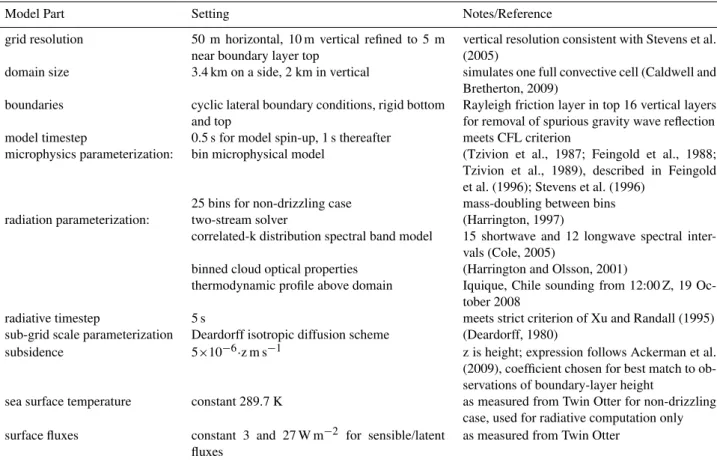
Fig. 1.Comparison of thermodynamic profiles between CIRPAS in-situ observations (data points) and LES output (lines). Observations show mean (symbol) and standard deviations (error bars) over each of the five flight legs. LES output are domain-averaged and temporally averaged over the sixth hour of simulation. Times of observations and LES output coincide.

thermodynamic profile from interpolation of profiles from McClatchy et al. (1971), as typically done in RAMS. Inter-polation between the McClatchy et al. (1971) subtropical winter and subtropical summer profiles by time of year was used to create an appropriate subtropical profile for 19 Oc-tober 2008. Latitudinal interpolation between that resulting profile and the McClatchy et al. (1971) tropical profile was used to create a profile appropriate for 20◦S.

Figures 1 through 3 show comparisons of profiles from the LES and observations. For the LES we show output from two simulations: one in which sub-grid diffusion of scalars (e.g. moisture, energy) is accounted for (DIFF); and one in which this sub-grid diffusion is neglected (NODIFF). Stevens et al. (2005), in a large LES intercomparison and per-formance study, suggest that neglecting the sub-grid diffu-sion of scalars leads to a more well-mixed model STBL and better agreement with observations by reducing the impact of over-entrainment common to LES. Nominally the sub-grid scheme ensures that fluxes of energy and moisture re-main constant with changes in model grid resolution; hence the primary disadvantage of neglecting sub-grid diffusion of scalars is that simulation output can exhibit dependency on changes in model grid resolution (Stevens et al., 2005). We deemed this possible modification to be acceptable if it re-sulted in better agreement between the model and obser-vations in our case. Furthermore, Cheng et al. (2010) have found that, even with the full use of the sub-grid scheme, boundary layer cloud LES output are resolution dependent.

Theθandqvprofiles as observed on the flight legs are

rea-sonably represented by the LES (Fig. 1a, b). Encouragingly, all model profiles show a well-mixed boundary layer simi-lar to that observed. For both simulations, domain-averaged model θ (by 0.1 K for DIFF and 0.2 K for NODIFF) and modelqv(by 0.24 g kg−1for DIFF and 0.21 g kg−1for

NOD-IFF, both by 3 %) in the boundary layer are biased low as

compared to the observations. Note that all quantitative com-parisons between model and observations are between plot-ted mean values only. The neglect of sub-grid diffusion of scalars leads to a small decrease inθand small increase inqv

within the boundary layer. This is expected because mixing of warmer and drier free tropospheric air into the boundary layer is reduced when this diffusion of scalars is neglected.

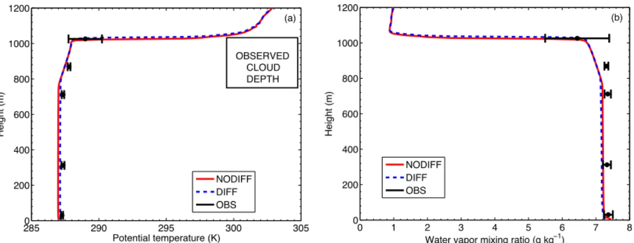
To determine how well the two LES configurations rep-resent observed dynamical properties, we examine resolved-scale profiles of vertical velocity variance, buoyancy produc-tion of turbulent kinetic energy (TKE) and total water flux. Vertical velocity variance (w′_w′_{), or the vertical component}

of TKE, is a useful proxy for the strength of circulations within the STBL. For the highest and lowest of the five air-craft altitudes (30 m and 1025 m), the DIFF and NODFF sim-ulations exhibit very little difference. In both cases, observed

w′_w′_{compares reasonably with modeled values. For the two}

flight legs at 710 and 870 m, observed values match well with NODIFF (underestimated by 8 %), and are underestimated by 24 % and 12 %, respectively, by DIFF. For the flight leg at 310 m altitude both simulations underestimatew′_w′_{by a}

fac-tor of 2 (by 54 % for DIFF and 46 % for NODIFF). NODIFF shows better agreement with observations, since this partic-ular configuration results in less entrainment of free tropo-spheric air and a smaller buoyancy sink of boundary layer TKE (Stevens et al., 2005). Thus more energy is available to drive STBL circulations.

(7)

0.0 0.1 0.2 0.3 0

200 400 600 800 1000

OBSERVED CLOUD DEPTH 1200

Vertical velocity variance (m2 s−2)

Height (m)

NODIFF DIFF OBS

Fig. 2.Comparison of resolved-scale flux profiles between CIRPAS in-situ observations (data points) and LES output (lines). Observa-tions show means (symbol) and computed errors (error bars) over each of the five flight legs. Errors are computed with propagation of measurement uncertainties in Table 2. LES output are domain-averaged and temporally domain-averaged over the sixth hour of simulation. Times of observations and LES output coincide.

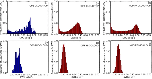
diffusion of scalars is neglected. This slight increase is ex-pected; less TKE is used to entrain potentially warmer air and mix it into the boundary layer (i.e. buoyancy destruction of TKE) when the entrainment rate is reduced. As we found in Fig. 2, the agreement between model and observations ap-pears reasonable in-cloud (overestimating by 7 % for DIFF and 25 % for NODIFF at 870 m) and poorer for the 300 m flight leg, underestimating by an order of magnitude in both cases. The observations in Figs. 2 and 3a suggest that parcels of air below cloud are more buoyant and lead to stronger up-drafts and downup-drafts in this region than what is simulated. Large-eddy simulation has been previously shown to under-estimate the strength of STBL circulations when compared to observations (e.g. Stevens et al., 2005).

The two simulations predict similar total water fluxes (Fig. 3b). Each simulation agrees quite well with observed values to within measurement uncertainty, although the ob-served total water fluxes are subject to substantial uncer-tainties due to instrument precision. Both simulations ex-hibit a positive increase in total water flux with height and as the cloud is entered. Total water flux within the STBL is slightly larger for NODIFF because there is more total wa-ter within the STBL (Fig. 1b) and because circulations are slightly stronger (Fig. 2).

To determine how well the model can represent the ob-served variation in cloud LWC, we compared the probabil-ity distribution functions (PDF) of LWC as observed on the flight legs near cloud top and mid-cloud to the PDF of LWC in similar layers (Fig. 4). The altitude of the Twin Otter var-ied by∼25 m and∼20 m on the two legs, respectively, and we computed the PDF of LWC with LES output for the same thickness layers.

The PDFs from observations at cloud top exhibits a modal value between 0.42 and 0.43 g kg−1with a long tail towards smaller values of LWC (Fig. 4a). The wide distribution of LWC values observed is due to the Twin Otter traversing both diluted (entrainment of overlying dry air is substan-tial) and undiluted (entrainment of overlying dry air is small) cloud parcels. At mid-cloud the width of the PDF is narrower (Fig. 4d) because at this height the cloud parcels are turbu-lently mixed and less entrainment of dry air occurs at this height. The modal value between 0.16 and 0.17 g kg−1is, as expected, lower than at cloud top.

The modeled distributions of LWC at cloud top compare reasonably well with observations. In general the PDFs from LES output (Fig. 4b, c, e, f) are less noisy because there are an order of magnitude more sampling points in the LES than in the flight leg (103in the observations vs. 104in the LES output). The similarity in PDF shape between the model output and observations is strong for DIFF (Fig. 4b). The modal value at cloud top is between 0.35 and 0.36 g kg−1, slightly (16 %) lower than that observed. At cloud top NOD-IFF (Fig. 4c) results in a modal value between 0.45 and 0.46 g kg−1 (neglecting zero LWC values), slightly higher (7 %) than that observed.

The two model predictions of the distribution of LWC mid-cloud both underestimate the modal value. For DIFF (Fig. 4e), the modal value mid-cloud (between 0.11 and 0.12 g kg−1) underestimates the observations by 30 %. The modal value between 0.15 and 0.16 g kg−1 for NODIFF (Fig. 4f) is underestimated by 6 % compared to the obser-vations. These differences in model output, paired with the errors at cloud top, suggest differing cloud thicknesses be-tween DIFF and NODIFF. The NODIFF simulation exhibits a thicker cloud layer than that of DIFF (265 m compared to 245 m).

It would be preferable to compare observed and simulated LWP. However, because the aircraft sampling strategy fo-cused mainly on horizontal legs it is not possible to generate statistically-significant observational estimates of LWP with-out assumption. If we assume an adiabatic profile of LWC in a 300 m thick cloud (as was observed), and set the cloud-top LWC value to the modal observed value, we derive an esti-mate for LWP in the observed case of 65 g m−2. From LES time series output, LWPs averaged over the simulated hour of observation for NODIFF and DIFF are 58.1 and 47.0 g m−2, respectively. Thus both simulations appear to underestimate observed LWP (9.9 % and 27.1 %, respectively).

(8)

−1.00 −0.5 0.0 0.5 1.0 1.5 200

400 600 800 1000 1200

Buoyancy production of TKE (m2_s−3_{* 10}−3₎

Height (m)

NODIFF DIFF OBS

−0.040 −0.02 0.00 0.02 0.04 −0.04 −0.02

200 400 600 800 1000 1200

OBSERVED CLOUD DEPTH

Total water flux (g kg−1 m s−1)

Height (m)

NODIFF DIFF OBS

(a) (b)

Fig. 3.Comparison of resolved-scale flux profiles between CIRPAS in-situ observations (data points) and LES output (lines). Observations show means (symbol) and computed errors (error bars) over the five flight legs. Errors are computed with propagation of measurement uncertainties in Table 2. LES output are domain-averaged and temporally averaged over the sixth hour of simulation. Times of observations and LES output coincide. The gray dashed line in(a)indicates zero values for visualization.

0.10 0.20 0.30 0.40 0.50 0.60 0.70 0.00

0.05 0.10 0.15

LWC (g kg )−1

Frequency of occurrence for LWC

OBS CLOUD TOP (a)

NODIFF CLOUD TOP (c)

0.10 0.20 0.30 0.40 0.50 0.60 0.70 0.00

0.05 0.10 0.15

LWC (g kg )−1

0.10 0.20 0.30 0.40 0.50 0.60 0.70 0.00

0.05 0.10 0.15

LWC (g kg )−1

OBS MID-CLOUD (d)

0.10 0.20 0.30 0.40 0.50 0.60 0.70 0.00

0.05 0.10 0.15

LWC (g kg )−1

0.10 0.20 0.30 0.40 0.50 0.60 0.70 0.00

0.05 0.10 0.15

LWC (g kg )−1

Frequency of occurrence for LWC 0.00 _{0.10 0.20 0.30 0.40 0.50 0.60 0.70} 0.05

0.10 0.15

LWC (g kg )−1

NODIFF MID-CLOUD (f) DIFF MID-CLOUD

(e) DIFF CLOUD TOP (b)

Fig. 4.Probability distribution function (pdf) of liquid water content observed with Phase Doppler Interferometer during flight leg at(a) cloud top, and(d)mid-cloud. These pdfs, as modeled with large-eddy simulation and allowing diffusion of scalars (DIFF) are shown in(b) (cloud top) and(e)(mid-cloud). The same, as modeled while neglecting diffusion of scalars (NODIFF), are shown in(c)(cloud top) and(f) (mid-cloud). Model output from large-eddy simulation is averaged over a 30 min window centered on time of observation (averaging over 6 snapshots at 5 min intervals). All liquid water contents are binned into 0.01 g kg−1ranges.

because of the better match between model output and ob-servations.

5 Experimental design

5.1 Determining meteorological and aerosol perturbations

In creating the experimental simulations for the comparative study, we required that variations in meteorological context

have three characteristics: (1) be constrained by observations, (2) be objectively computed, and (3) be determined consis-tently. In some modeling sensitivity analyses, large pertur-bations in variables are purposely chosen to maximize the possibility of finding a response. We prefer the perturbations to be more realistic so that the response of the stratocumu-lus cloud system to one perturbation can be reasonably com-pared with another.

To determine realistic perturbations in theqtandθjumps

(9)

10 11 12 13 14 15 0

200 400 600 800 1000 1200 1400

Time (UTC)

Solar insolation at TOA (W m

−2)

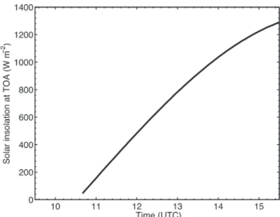
Fig. 5.Solar insolation at TOA as it varies over simulation time for the base case LES. All experimental simulations have the same solar insolation as the base case.

use the ERA-Interim dataset (Uppala et al., 2005, 2008). We chose to use the ERA-Interim data because the ECMWF family of models gives a reasonable match to satellite-observation monthly mean low cloud fractions in our region of interest (Wyant et al., 2010). We note this match in cloud fractions is somewhat poorer near our region of interest, as are matches in some other properties such as boundary layer depth (Wyant et al., 2010). The ERA-Interim data is also spa-tially coarse as compared to available observations. However, it give us a far larger temporal variation in meteorology than we would obtain from the observations taken from the Twin Otter during VOCALS (19 flights, 2 soundings taken per flight). This variation is of importance to our study because it helps to expand the applicability of our results to South-east Pacific coastal stratocumulus outside of those observed during VOCALS. It is prudent to compare our computed per-turbations inqtandθjumps to the variations observed from

the Twin Otter (Zheng et al., 2011), and we do so below. We first accumulated daily reanalysis data from the two nearest available reanalysis data points to 20◦_{S, 72}◦_W,

where the Twin Otter conducted all its flights (20.0◦_S,

72.4◦_{W and 20.0}◦_{S, 71.7}◦_{W). The data is gridded at 2.5}◦_by

2.5◦latitude-longitude resolution at six-hour intervals. From the surface (1000 mb) to an altitude of 700 mb, the vertical resolution is 25 mb. We used all days from September to November from 2001 to 2010 since stratocumulus is persis-tent during the austral spring in this region. We used 18:00 Z data since this time most closely coincides with the observa-tions.

Although stratocumulus is persistent in the observed re-gion during the austral spring, the stratocumulus layer can be subjected to synoptic changes that influence its robustness (Rahn and Garreaud, 2010). To ensure that a stable stratocu-mulus layer existed around 20◦_{S, 72.5}◦_{W for all reanalysis}

data we excluded data on days when the low cloud fraction was below 0.95 at either of the two reanalysis data points at either 12:00 and 18:00 Z.

To ensure that the reanalysis data exhibit spatial homo-geneity around 20◦_{S, 72.5}◦_{W, we also excluded days where}

the height of the inversion (height of the steepest gradients in temperature and water vapor mixing ratio) did not coincide between the two grid points. Using these strict criteria, we were left with 60 data points from which to compute pertur-bations.

The ERA-Interim data is of too coarse a vertical resolu-tion (25 mb) to resolve the inversion jump. For this reason we computed the jump properties as the maximum gradi-ent across two 25 mb vertical layers (over 50 mb, or roughly 0.5 km) between the 1000 and 700 mb levels. With this ap-proach we avoid the 25 mb layer wherein the inversion is represented, and obtain the total change inθ andqt across

the boundary layer top for our 60 data points.

From this accumulated data set we computed the standard deviation forθ andqtjumps across the cloud top interface.

Note that the mean values of the jump values within the ERA-Interim data we select do not coincide with the mean values in the model base case. It is the variationof these jumps within the ERA-Interim data that is of interest, and from which we determine the perturbations we use in our modeling framework.

To modify theqt andθ jumps above the boundary layer

in the experimental simulations, we altered the properties of the model free troposphere instead of the properties of the model boundary layer. We first determined the height of the model boundary layer as the model layer for which the liq-uid water potential temperature gradient was maximized for each model column in the domain. We then modified the in-stantaneous values ofqvorθ for all model layers above the

boundary layer.

For the simulations where theθ jump was modified, we increased and decreased theθ above the boundary layer by one standard deviation (UP THETA and DOWN THETA,

±1.3 K). Because the observed free troposphericqv is low

(below 1.0 g kg−1), the two perturbations for the qt jump

were both in the positive direction; by one standard deviation (UP MOIST,+0.87 g kg−1) and by two standard deviations (UP 2XMOIST,+1.74 g kg−1).

We compared our computed perturbations inqtandθjump

to the variations in these jumps observed from the Twin Otter (see Zheng et al., 2011, Table 2). Our computed jump inθ

is smaller by 0.7 K (±1.9 K observed), while our computed jump inqtsmaller by more than a factor of two (±2.2 g kg−1

observed). The ERA-Interim data may not capture the free tropospheric variability observed from the Twin Otter during VOCALS. Our possible underestimation of the magnitude of

qt and θ variabilities could lead to underestimation of the

associated cloud response.

(10)

Table 4.Aerosol and meteorological properties varied and for which the response of cloud properties LWP, optical depth and cloud radiative forcing are computed.

Factor Modify by Possible impacts on STBL References

Aerosol concentration Half/quarter value uniformly across size distribution

Alters aerosol-cloud interactions

refer to introduction

Moisture jump Increase moisture content above BL by [1,2]·0.87 g kg−1

Modulates evaporation through entrainment mixing

Ackerman et al. (2004)

Potential temperature jump Increase/decrease potential temperature above BL by 1.3 K

Modulates energy

transfer through and amount of entrainment mixing

Lilly (1968); Sullivan et al. (1998)

variation in aerosol state, acknowledging that rigorous cor-respondence does not exist between our meteorological and aerosol perturbations.

We chose to perturb only total aerosol concentrationNa,

with no change in the mean particle size Dp (0.12 µm).

The simulated change in cloud drop concentration corre-lates strongly with the aerosol concentration perturbations. The initial mean values of model Na and Nd in the base

case (Na=450 cm−3,Nd=425 cm−3) represent a strongly

polluted stratocumulus case with substantial activation of aerosol. As a result, we elected not to impose an increase in aerosol concentration as a perturbation. Instead, we main-tain the same aerosol size distribution shape and decrease the aerosol concentration by factors of 2 and 4 , thereby simulating moderately polluted (HALF ND) and fairly clean (QUARTER ND) STBL cases, respectively. The lowest val-ues ofNa=113 cm−3,Nd=106 cm−3are fairly

representa-tive of the clean STBL (Miles et al., 2000).

In order to span the full range of aerosol and cloud droplet concentrations observable within stratocumulus, a lower-end value ofNd=50 cm−3is probably more appropriate, while

the upper rangeNd=425 cm−3is a reasonable upper value.

Although we do not have decadal time series of aerosol data available for the region of interest, we note that the Twin Otter observedNdto vary between 80 cm−3and 400 cm−3

during VOCALS (Zheng et al., 2011). Thus our selectedNd

range is reasonable compared to the available observations. The aerosol and meteorological properties that are var-ied, the magnitude of these variations, and possible ways in which the cloud will respond to these variations, are sum-marized in Table 4. We focused on the response of stratocu-mulus to those meteorological factors likely to modify STBL evolution on time scales less than a day.

5.2 Configuration of experimental simulations

By perturbing the base simulation with one perturbation at a time from Table 4 (two different perturbations of one aerosol and each of two meteorological properties), we cre-ated six separate experimental simulations. The perturba-tions described in the previous subsection were added at 09:30 UTC, two hours into the base LES, and the

simula-tions were allowed to run for an additional six hours, to 15:30 UTC. At this time the cloud layer begins to break up. Simulating this time period allows us to determine how the responses of LWP, τ and CRF for overcast stratocumulus vary through the observation period to near solar noon. For reference, Fig. 5 shows the temporal variation of solar inso-lation at TOA for the base simuinso-lation.

As noted above, meteorological context and aerosol state are often correlated (Brenguier et al., 2003). Independent meteorological variables are also often correlated with each other. Here we assume independence because attributing changes in cloud properties1cto changes in specific aerosol and meteorological factors will be simpler if we only con-sider factors one at a time. Interactions between two or more co-varying properties would make the attribution process more difficult. Examining changes in the cloud response to co-varying aerosol and meteorological properties is left to future study, possibly using the factorial method (Teller and Levin, 2008).

6 Results from experimental simulations

We first briefly describe the time evolution of the cloud layer in the model base case to provide some context for the dis-cussion of the perturbation simulations. From 09:30 UTC to 15:30 UTC, the base case LWP decreases from 67 g m−2 to 18 g m−2as solar insolation increases. After 14:00 UTC the cloud layer has thinned such that it is optically thin in the longwave (LW) (Garrett and Zhao, 2006; Petters et al., 2012), and LW radiative cooling from the cloud top begins to de-crease slightly with time.

Cloud fraction, defined as the ratio of model columns with LWP<10 g m−2to the total number of model columns, de-parts from unity shortly after 14:00 UTC and decreases to

(11)

20 40 60 80 100 120

10 11 12 13 14 15

Time (UTC)

Liquid water path (g m )

−2 BASE

UP THETA DOWN THETA

800 850 900 950 1000 1050

Boundary layer top (m)

40 45 50 55 60 65 70 75 80

Int. cloud longwave cooling (W m )

−2

(a)

(b)

(c)

BASE UP THETA DOWN THETA

10 11 12 13 14 15

Time (UTC)

10 11 12 13 14 15

Time (UTC)

285 290 295 300 305

−1.00 −0.5 0.0 0.5 1.0 1.5 200

400 600 800 1000 1200

Height (m)

0 10 20 30 40 50 60 70 80 90 100 110

Int. cloud shortwave heating (W m )

-2

(d) (e) (f)

BASE UP THETA DOWN THETA

10 11 12 13 14 15

Time (UTC) Buoyancy production of TKE (m s ) x 102−3 −3 0 200 400 600 800 1000 1200

Height (m)

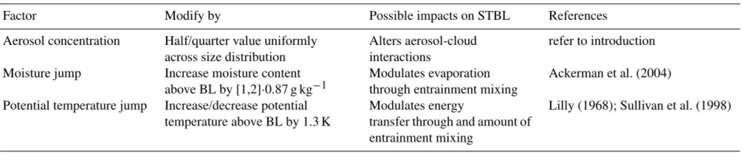
Fig. 6.LES output showing STBL response for changes in potential temperature jump across the cloud top interface. Time series of quantities, shown in(a)to(d), are domain averaged and vertically integrated. Vertical profiles, shown in(e)and(f), are domain averaged and temporally averaged over the hour of observation (12:30 to 13:30 UTC).

of the experimental simulations, even in those where cloud droplet concentrations were reduced.

6.1 Response to perturbations in potential temperature jump

Perturbations in the θ jump from the base case (labeled BASE) lead to changes in entrainment rate that affect cloud LWP. Together Fig. 6a, f show that an increase in theθabove the STBL leads to a higher LWP and vice versa (simulations UP THETA and DOWN THETA, respectively).

As suggested by other studies (e.g. Lewellen and Lewellen, 1998; Sullivan et al., 1998; Sun and Wang, 2008), an increase in the θ jump leads to stronger stability (i.e. greater density contrast) across the interface, reducing the rate at which dry air from above the cloud top entrains into the boundary layer. Also, because of the increase inθabove the boundary layer, cloud integrated LW radiative cooling is reduced (Fig. 6c) and hence there is less buoyant production of TKE within the cloud layer (Fig. 6e). Buoyant production is the primary source of TKE within the convective STBL, and a decrease in this quantity results in less TKE available to drive entrainment. Taken together, these two mechanisms lead to a slower increase in boundary layer height (Fig. 6b). Boundary layer height is directly related to entrainment rate because large-scale subsidence is the same in all simulations (see Table 1).

The converse of these qualitative arguments applies when theθjump is decreased. However, the cloud response is not identical in magnitude for the positive and negativeθjumps, i.e. the response is not symmetric.

As the sun rises toward mid-day and cloud integrated SW radiative heating increases (Fig. 6d), LWP decreases in all three simulations. Shortwave radiative heating increases with LWP and explains in part why the LWP for the UP THETA simulation decreases more rapidly after 13:00 UTC as com-pared to the other two. Integrated LW cooling also decreases after 13:00 UTC in all three simulations as the cloud layer becomes optically thin in that portion of the electromagnetic spectrum.

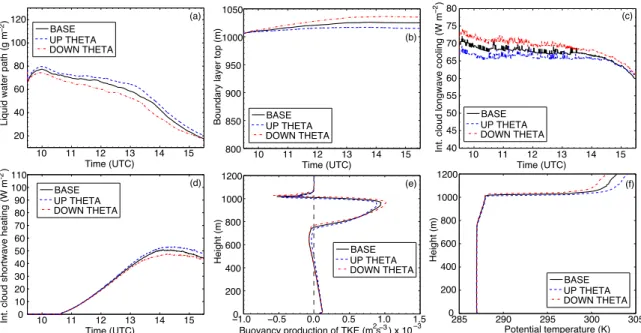
6.2 Response to perturbations in moisture jump

For the base case, decreases in the magnitude of theqtjump

(i.e. moistening the free troposphere) lead to increases in LWP (Fig. 7a, f). Like the STBL response to changes in theθ

jump, changes in LWP are related to changes in the entrain-ment process and the magnitude of LW radiative cooling. For the same amount of entrained overlying air into the STBL, increasingqvabove the boundary layer leads to less

evapo-ration of cloud and less associated evaporative cooling. This change in the entrainment process partly explains both the increase in LWP with increasing free troposphericqt, as well

as the increase in latent heating at cloud top (Fig. 7d). Simul-taneously, integrated LW radiative cooling decreases as there is more water vapor to emit LW radiation to the top of the cloud (Fig. 7c).

As in Fig. 6, this decrease in integrated LW cooling (in conjunction with less cloud top evaporative cooling) leads to less buoyancy production of TKE (Fig. 7e) when the magnitude of the qt jump decreases. Again, as this

(12)

−1.0 −0.5 0.0 0.5 1.0

−15 −10 −5 0 5

Latent heating (K hr )−1 0 Water vapor mixing ratio (g kg )2 4 6 −1 8

(a) (b) (c)

(d) _(e) (f)

BASE UP MOIST UP 2XMOIST

Buoyancy production of TKE (m s ) x 102−3 −3 40 45 50 55 60 65 70 75 80

−2

10 11 12 13 14 15

Time (UTC)

10 11 12 13 14 15

Time (UTC) 10 11 Time (UTC)12 13 14 15

800 850 900 950 1000 1050

20 40 60 80 100 120

−2

0 200 400 600 800 1000 1200

Height (m)

0 200 400 600 800 1000 1200

Height (m)

0 200 400 600 800 1000 1200

Height (m)

Fig. 7.LES output showing STBL response for changes in moisture jump across the cloud top interface. Time series of quantities, shown in (a)to(c), are domain averaged and vertically integrated. Vertical profiles, shown in(d)to(f), are domain averaged and temporally averaged over the hour of observation (12:30 to 13:30 UTC).

entrainment rate, which can be seen as a reduction in bound-ary layer growth (Fig. 7b). This reduction in entrainment rate with increased free troposphericqtalso leads to less

evapo-ration of cloud. There is less mixing of relatively dry overly-ing air into the cloud, and what mixoverly-ing does occur broverly-ings in moister cloud-free air.

Different from the perturbations inθjump, one of the sim-ulations, UP 2XMOIST, does not appear to become optically thin in the LW spectrum near the end of simulation. Inte-grated LW radiative cooling decreases only slightly at the end of simulation, whereas for the other two (BASE and UP MOIST) LW cooling decreases more substantially (Fig. 7c). Furthermore, comparing Fig. 6a to Fig. 7a shows that the re-sponse of LWP to the moisture jump perturbations is larger than the response toθjump perturbations. This difference in LWP response has important bearing on the associated re-sponse ofτ and CRF.

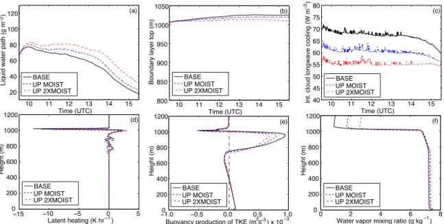
6.3 Response to perturbations in aerosol concentration

Previous studies have shown that perturbations in Na and Nd can lead to either cloud thinning or thickening. When

large scale forcings such as subsidence and SW forcing are held constant, changes in either the drizzle process (Albrecht, 1989; Jiang et al., 2002) or the entrainment process (Acker-man et al., 2004; Bretherton et al., 2007; Hill et al., 2009) can each play important roles in the STBL response. We found that, compared to our descriptions of cloud response to the meteorological perturbations, accurate description of how perturbations toNa andNd impact the simulations

re-quires more elaboration.

Relative to the base case, decreases inNaandNdlead to

increases in LWP (Fig. 8a). Increases in LWP with decreases inNaandNdoccur almost immediately after the aerosol

per-turbations were introduced at 09:30 UTC. What is the mecha-nism causing the immediate divergence in model LWPs with changes inNaandNd? Because the thermodynamic profiles

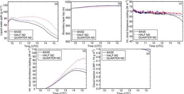
of all three simulations are identical immediately after the aerosol perturbations are introduced, it is unlikely that ther-modynamics play a role in the immediate response (though feedbacks to the thermodynamic state could strongly affect the longer time-scale response). Instead we look to immedi-ate changes in microphysical processes when cloud droplet concentration is altered (Fig. 9).

Our simulations exhibit a weak drizzle process. Even when

Ndis decreased to its lowest value in QUARTER ND there

is negligible sedimentation of cloud water below cloud base (not shown). Thus we look to potential changes in the en-trainment process. When cloud droplet concentration is creased evaporative cooling at cloud top is expected to de-crease for two reasons: there is less total droplet surface area through which liquid water can become water vapor (Wang et al., 2003; Ackerman et al., 2004; Hill et al., 2009), and there are fewer droplets near the cloud top interface because larger droplets sediment faster (Bretherton et al., 2007; Hill et al., 2009).

As the evaporation rate near cloud top decreases, LWP would be expected to increase. We see that, for the first half hour after perturbations are induced, evaporative cool-ing (negative latent heatcool-ing) at cloud top (associated with entrainment) does decrease with decreases in Na and Nd

(13)

(a) (b) (c) (d) (e) BASE HALF ND QUARTER ND BASE HALF ND QUARTER ND BASE HALF ND QUARTER ND BASE HALF ND QUARTER ND BASE HALF ND QUARTER ND

10 11 12 13 14 15

Time (UTC)

10 11 12 13 14 15

Time (UTC)

10 11 12 13 14 15

Time (UTC)

10 11 12 13 14 15

Time (UTC)

10 11 12 13 14 15

Time (UTC) 0 10 20 30 40 50 60 70 80 90 100 110

Int. cloud shortwave heating (W m )

-2 0.0 0.1 0.2 0.3 0.4 0.5 0.6 0.7 0.8 0.9 1.0

Cloud fraction (LWP < 10 g m )

−2 20 40 60 80 100 120

−2 800 850 900 950 1000 1050

40 45 50 55 60 65 70 75 80

−2

Fig. 8.LES output showing STBL response for changes in aerosol and cloud droplet concentrations. Domain averaged and vertically inte-grated time series of quantities are shown.

−1.5 −1.0 −0.5 0.0 0.5 1.0 1.5 2.0

(e) (f)

(d)

(a) (b) (c)

BASE HALF ND QUARTER ND BASE HALF ND QUARTER ND BASE HALF ND QUARTER ND BASE HALF ND QUARTER ND BASE HALF ND QUARTER ND BASE HALF ND QUARTER ND

Buoyancy production of TKE (m s ) x 102−3 −3

0.0 0.1 0.2 0.3 0.4 0.5 0.6

Vertical velocity variance (m s )2−2

0.0 0.1 0.2 0.3 0.4 0.5 0.6

Vertical velocity variance (m s )2−2

290 295 300 305

0 200 400 600 800 1000 1200 Height (m) 285 0 200 400 600 800 1000 1200 Height (m) 0 200 400 600 800 1000 1200 Height (m) 0 200 400 600 800 1000 1200 Height (m) 0 200 400 600 800 1000 1200 Height (m) 0 200 400 600 800 1000 1200 Height (m)

0 2 4 6 8

Water vapor mixing ratio (g kg )−1

−15 −10 −5 0 5

Latent heating (K hr )−1

Fig. 9.LES output showing STBL response for changes in aerosol and cloud droplet concentrations. Vertical profiles, shown in(a)to(c), are domain averaged and temporally averaged over the first fifteen minutes of simulation after perturbation (09:30 to 09:45 UTC). Vertical profiles, shown in(d)to(f), are domain averaged and temporally averaged over the hour of observation (12:30 to 13:30 UTC).

be related to the increases in LWP seen in Fig. 8a immedi-ately after 09:30 UTC.

Less evaporative cooling at cloud top also causes less buoyancy production of TKE in that region (Fig. 9c), re-sulting in decreases inw′_w′_{near cloud top (Fig. 9b, around}

800 m altitude). Weaker turbulence leads to less vigorous en-trainment, and thereby larger LWP can be maintained. As a whole this process is known as the evaporation-entrainment

effect (Hill et al., 2009). This effect could also play a role in the immediate increases in LWP with decreased Nd at

09:30 UTC.

(14)

12 13 14 15

−30 −25 −20 −15 −10 −5 0

5

10

Time (UTC)

LWP response to perturbation (g m

−2)

THETA MOIST ND

10 20 30 40 50 60 70 80 90

Liquid water path (g m

−2)

Fig. 10.Response of LWP to perturbations in meteorological con-text and aerosol state, computed from the experimental simulations (left y-axis). All mean responses are computed using 5-min tem-porally and domain averaged data, averaged over each of the four hours. Standard deviations for these means are shown with error bars. The grey dashed line indicates a zero response in LWP. The hour over which we average is the same for each computed re-sponse; we spread the responses out around each time for clarity. There are two computed hourly responses for each perturbation type; refer to Table 5 for exact expressions. For reference the black line shows the time series of base case LWP (right y-axis).

of entrainment efficiency (Bretherton et al., 1999). We antici-pate this overestimation to somewhat exaggerate the strength of cloud top evaporation and its dependence onNaandNd.

We also find that, in response to the evaporation-entrainment effect, boundary layer growth decreases with de-creases inNd (Fig. 8b) as entrainment rate decreases. This

change in boundary layer growth plays an important role in the further evolution of these simulations. Before we elab-orate further, we first consider the impacts of LW radiative cooling and SW radiative heating.

Figure 8c shows us that integrated LW cooling is simi-lar across all three simulations until about 13:30 UTC. After 13:30 UTC we see that LW cooling is dependent onNddue to

variations in cloud thinning and reductions in cloud fraction withNd(Fig. 8e). After this time, asNddecreases, integrated

LW cooling increases because the cloud fraction increases and individual cloudy model columns are more likely to be optically thick in the LW. This change in LW cooling with

Nd could help explain the slight increase in differences in

LWP across the three simulations after 13:30 UTC; more LW cooling within the boundary layer can lead to cloud growth through a lowering of the lifting condensation level.

Decreases in Nd lead to more integrated SW heating

(Fig. 8d). Because cloud integrated SW heating increases with increases in both LWP andNd, it is clear that the

in-crease in LWP and consequent inin-crease in cloud SW heating dominates the expected decrease in SW heating due to de-creases in Nd. If SW heating were to play a primary role,

we would expect LWP values across the simulations to be-come more similar during the day because higher LWP

val-12 13 14 15

−5 −4 −3 −2 −1 0 1 2 3 4 5

Time (UTC)

Optical Depth response to perturbation

THETA MOIST ND

4 6 8 10 12 14 16 18

Optical Depth

Fig. 11.Response of optical depth (τ) to perturbations in meteoro-logical context and aerosol state, computed from the experimental simulations (left y-axis). Responses ofτare shown as described in Fig. 11. For reference the black line shows the time series of base caseτ (right y-axis) and the grey dashed line indicates a zero re-sponse inτ.

ues beget more heating and would lead to more cloud evap-oration. Because we do not find this relationship between LWP andNd(Fig. 8a), we turn to the role of boundary layer

growth and entrainment to explain the simulated longer-term response to aerosol.

Averaged over the fourth hour of simulation after the per-turbations were induced (12:30 to 13:30 UTC),qvandθ

pro-files indicate that, asNd decreases, a cooler, moister STBL

results (Fig. 9d, e) that leads to more cloud growth. This cooler, moister STBL can be attributed to slower boundary layer growth and entrainment (Fig. 8b); more entrainment of warm, dry overlying air leads to a warmer, drier STBL. Note that Fig. 9d and e are qualitatively representative of adjacent hourly periods for these simulations.

Although the differences are small, we see near cloud top (900 m to 1000 m) for the hour between 12:30 and 13:30 UTC thatw′_w′ _{is smaller for the lower values of}_N

d

(Fig. 9f). This relationship can again be associated with the evaporation-entrainment feedback, as we found near cloud top from 09:30 UTC to 09:45 UTC (Fig. 9b). This relation-ship between circulation strength and Nd near cloud top is

in contrast with the more obvious increase ofw′_w′_with

de-creases inNd for the bulk of the STBL. However, we must

keep in mind the importance of circulation strength near cloud top in determining entrainment rate, as opposed to cir-culation strength through the boundary layer (Lilly, 2002; Caldwell and Bretherton, 2009). Taken as a whole, and as seen in Wang et al. (2003), Figs. 8 and 9 show that decreases in evaporative cooling and entrainment rate with decreases in

NaandNdresult in the increases of LWP found in this set of

(15)

Table 5.Expressions depicting how the two hourly-averaged responses (leftmost and rightmost for each hour) are computed for each pertur-bation in Fig. 10 to 13. The expressions in the rightmost column use the simulation names described in Sect. 5.

Perturbation Left-hand Right-hand

Aerosol concentration (HALF ND)–(QUARTER ND) (BASE)–(HALF ND)

Moisture jump (UP MOIST)–(UP 2XMOIST) (BASE)–(UP MOIST)

Potential temperature jump (BASE)–(DN THETA) (UP THETA)–(BASE)

12 13 14 15

−2.0 −1.5 −1.0 −0.5 0.0 0.5 1.0 1.5

Time (UTC)

LW CRF surface (W m )

−2

75 76 77 78 79

80

81 82 83 84 85

12 13 14 15

−0.4 −0.2 0.0 0.2 0.4 0.6 0.8 1.0

Time (UTC)

CRF response to perturbation (W m )

−2

THETA MOIST ND

(a) (b)

LW CRF TOA (W m )

−2

20.0 20.5 21.0 21.5 22.0

−2

THETA MOIST ND

Fig. 12.Response of longwave cloud radiative forcing (LW CRF), at(a)TOA and(b)the surface to perturbations in meteorological context and aerosol state, computed from the experimental simulations (left y-axis). Responses of LW CRF are shown are shown as described in Fig. 11. For reference the black line shows the time series of base case LW CRF (right y-axis) and the grey dashed line indicates a zero response in LW CRF.

7 The computed response in cloud properties

To objectively compare the impact of the perturbations in meteorological context 1m and aerosol state 1a on the model base case, we computed the response of three cloud properties 1c (LWP, τ and CRF) to these perturbations. We computed these responses from 5-min domain averaged cloud properties, averaged over one hour centered on each of the last four hours of simulation (12:00, 13:00, 14:00 and 15:00 UTC).

Because we have two separate perturbations (e.g. UP THETA and DOWN THETA) for each of the three per-turbed parameters, we computed two hourly-averaged cloud responses for each hour.

For all perturbation types, the two responses are reported by comparing cloud properties for (i) the simulations using themiddle(absolute) value ofθ jump,qtjump, andNa and Ndrelative to the simulation usingsmallestvalue, and then

(ii) by comparing the simulations using thelargestperturbed parameter value relative to themiddlevalue. See Table 5 for the exact choice of simulations used for each response calcu-lation.

Figures 10 to 13 show these computed responses. While the hour over which we average is the same for all responses, we slightly shift the results left or right at each hour for clar-ity. As shown in Table 5, at each hour in Figs. 10 to 13 the point slightly shifted to the left is for the middle–smallest simulations, while the point shifted to the right is for the largest–middle simulations.

7.1 The response to changes in jump properties compared to the response to changes in droplet concentration

7.1.1 Liquid water path

Figure 10 shows the time evolution of the response of LWP. Averaged over the two responses at each hour and across all four hours, the LWP response to increases in Nd is the

largest in magnitude (−13 g m−2), followed by the response to increases in theqtjump (−8 g m−2). The average LWP

re-sponse to increases in theθjump is the smallest at 5 g m−2. For each perturbation, the LWP response varies with hour and, in some cases, at each hour between the two perturba-tions (e.g. UP THETA and DOWN THETA). The LWP re-sponse to increases in theθ jump is positive and varies the least over simulation time (between 2 and 7 g m−2). The LWP response to increases in theqt jump (decrease in free

tropo-sphericqt is negative, varying between−5 and−12 g m−2.

Within each hourly average, the LWP response to changes inθ jump is fairly linear (e.g. the response at each hour for UP THETA and DOWN THETA are similar). For changes in theqtjump, the LWP response is fairly linear at 12:00 and

13:00 UTC and less so at 14:00 and 15:00 UTC.

The LWP response to increases in Nd is negative and

varies between −6 and −23 g m−2. For all four hours we find a non-linear LWP response to these increases inNd. The

first increase fromNd=106 cm−3toNd=213 cm−3yields

(16)

−30 −20 −10 0 10 20 30 40 50 60 70

−450 −400 −350 −300 −250 −200 −150

(a) (b)

−40 −20 0 20 40 60 80

−450 −400 −350 −300 −250 −200 −150

−2

SW CRF surface (W m )

−2

SW CRF TOA (W m )

−2

12 13 14 15

Time (UTC) 12 13Time (UTC)14 15

THETA MOIST ND

Fig. 13.Response of shortwave cloud radiative forcing (SW CRF), at(a)TOA and(b)the surface to perturbations in meteorological context and aerosol state, computed from the experimental simulations (left y-axis). Responses of SW CRF are shown as described in Fig. 11. For reference the black line shows the time series of base case SW CRF (right y-axis) and the grey dashed line indicates a zero response in SW CRF.

changes in entrainment rate with Nd (Fig. 8b). This

non-linearity increases with time.

Because of the substantial decrease in LWP during the day, relative LWP response varies more widely with time as com-pared to absolute LWP responses. For example, relative LWP responses to increases inNdvary from−10 % at 12:00 UTC

to−94 % at 15:00 UTC, when the cloud layer is thinnest.

7.1.2 Optical depth

We found the LWP response to changes in meteorologi-cal perturbations (1m) to be of the same magnitude, or smaller, than the LWP response to aerosol perturbations (1a) (Fig. 10). However, the LWP response to these perturbations can not be directly translated into radiative responses. In gen-eral bulk optical depthτ is proportional to LWP,Ndand the

dispersion of the cloud drop size distribution, represented by

k(Brenguier and Geoffroy, 2011):

τ∼(kNd)1/3LWP5/6. (1)

We computedτ for the SW portion of the spectrum using:

τ= zt Z

zb ru Z

rl

2π r2n(r)drdz, (2)

wherezt andzbare the heights of the cloud top and cloud

base, respectively,ruandrl are the radius size range of the

drop size distribution andn(r) is the number of drops be-tweenrandr+dr(Seinfeld and Pandis, 1998). The extinc-tion efficiency is assumed to be 2. Using output of 5-min av-eraged cloud droplet size distribution data, we integrated the model drop size distribution first over the 25 bins in the mi-crophysical model and then over the total depth of the cloud layer. For the base case, changes inτ with time follows the same trend as LWP with time (compare the black lines on Fig. 10 and Fig. 11), as expected from Eq. (1).

The optical depth response to perturbations in the two jump properties is proportional to LWP responses (Fig. 11).

For increases in qt jump strength, hourly-averaged values

of this response in τ are between −2.7 (−25 %) to −1.0 (−15 %). For increases inθjump strength, hourly-averaged values ofτincrease by 0.7 (11 %) to 1.5 (8 %). Note that rela-tive response inτis computed relative to their corresponding “BASE” hourly-averagedτ values.

Comparison of the response in τ to Nd perturbations

(Fig. 11) to the concurrent response in LWP (Fig. 10) re-veal substantial differences. We find that the response inτ

changes both sign and magnitude over simulation time when

Nd is increased. At 12:00 UTC the hourly-averaged τ

re-sponse, averaged over the two responses for that hour, is 1.6 (10 %). This response decreases to 0.6 (4 %),−0.6 (−6 %), and finally−1.2 (−18 %) for 15:00 UTC. In contrast, pertur-bations inNdelicited a negative LWP response throughout

simulation time.

We find the response ofτto increases in both jump proper-ties to also be proportional to the response of LWP. Increases inqtjump strength (decrease in free troposphericqt)

primar-ily lead to decreases in LWP andτ, and increases in theθ

jump strength primarily lead to increases in LWP andτ. In both cases,Ndremains relatively unchanged. When we

per-turbNd, we do not find this same direct proportionality

be-tween LWP andτ. In general, increasingNdin stratocumulus

while holding other properties constant leads to an increase inτ(Twomey, 1977), as shown in Eq. (1). The LWP response to increasingNdis negative (Fig. 10), the result of which is

a decrease in τ. When taken together the two separate ef-fects on τ somewhat mitigate each other. This mitigation, or cancellation, has been found in other modeling studies of aerosol-cloud interactions within both marine stratiform (Ackerman et al., 2004; Wood, 2007) and marine cumuliform (Zuidema et al., 2008) cloud layers. In the simulations, the response ofτ to increasingNdis dominant at 12:00 UTC but

becomes less so as the simulation continues. By 15:00 UTC impact of increasingNdis more than offset by the response

of τ to the decrease in LWP, resulting in a net negative τ