A comparative study of the response of non-drizzling stratocumulus to meteorological and aerosol perturbations

(1)

ACPD

12, 27111–27172, 2012

Stratocumulus response to perturbations

J. L. Petters et al.

Title Page

Abstract Introduction

Conclusions References

Tables Figures

◭ ◮

Back Close

Full Screen / Esc

Printer-friendly Version Interactive Discussion

Discussion

P

a

per

|

Dis

cussion

P

a

per

|

Discussion

P

a

per

|

Discussio

n

P

a

per

|

Atmos. Chem. Phys. Discuss., 12, 27111–27172, 2012 www.atmos-chem-phys-discuss.net/12/27111/2012/ doi:10.5194/acpd-12-27111-2012

Atmospheric Chemistry and Physics Discussions

This discussion paper is/has been under review for the journal Atmospheric Chemistry and Physics (ACP). Please refer to the corresponding final paper in ACP if available.

A comparative study of the response of

non-drizzling stratocumulus to

meteorological and aerosol perturbations

J. L. Petters1, H. Jiang2, G. Feingold3, D. L. Rossiter1, D. Khelif4, L. C. Sloan1,

and P. Y. Chuang1

1

University of California – Santa Cruz, Santa Cruz, USA 2

Cooperative Institute for Research in the Atmosphere, Fort Collins, USA 3

NOAA/Earth System Research Laboratory, Boulder, USA 4

University of California – Irvine, Irvine, USA

Received: 4 September 2012 – Accepted: 8 September 2012 – Published: 16 October 2012

Correspondence to: J. L. Petters (jlpetter@ucsc.edu)

(2)

ACPD

12, 27111–27172, 2012

Title Page

Tables Figures

◭ ◮

Back Close

Full Screen / Esc

Discussion

P

a

per

|

Dis

cussion

P

a

per

|

Discussion

P

a

per

|

Discussio

n

P

a

per

|

Abstract

The impact of changes in aerosol and cloud droplet concentration (NaandNd) on the

radiative forcing of stratocumulus-topped boundary layers (STBLs) has been widely studied. How these impacts compare to those due to variations in meteorological context has not been investigated in a systematic fashion. In this study we

exam-5

ine the impact of observed variations in meteorological context and aerosol state on daytime, non-drizzling stratiform evolution, and determine how resulting changes in cloud properties compare. We perturb aerosol and meteorological properties within an observationally-constrained LES and determine the cloud response, focusing on changes in liquid water path (LWP), bulk optical depth (τ) and cloud radiative forcing

10

(CRF).

We find that realistic variations in meteorological context (i.e. jump properties) can

elicit responses inτand shortwave (SW) CRF that are on the same order of magnitude

as, and at times larger than, those responses found due to similar changes in aerosol

state (i.eNd). Further, we find that one hour differences in the timing of SW radiative

15

heating can lead to substantial changes in LWP andτ. Our results suggest that, for

ob-servational studies of aerosol influences on the radiative properties of stratiform clouds, consistency in meteorological context (the cloud top jump properties in particular) and time of observations from day-to-day must be carefully considered.

1 Introduction

20

Marine boundary layer stratiform clouds are persistent and prevalent (Klein and Hart-mann, 1993), imparting a strong negative forcing to the Earth’s radiative budget (Chen et al., 2000). The representation of these clouds in current climate models is relatively poor, leading to large uncertainty in climate projections (Randall et al., 2007). The dif-ficulty in representing stratiform clouds in large-scale models is exacerbated by their

(3)

ACPD

12, 27111–27172, 2012

Title Page

Tables Figures

◭ ◮

Back Close

Full Screen / Esc

Discussion

P

a

per

|

Dis

cussion

P

a

per

|

Discussion

P

a

per

|

Discussio

n

P

a

per

|

sensitivity to changes in aerosol state and in the “meteorological context” in which the cloud system resides.

The impacts of perturbations in aerosol state on the radiative properties of stratiform cloud systems have been widely studied. These studies have focused on changes in cloud optical properties (e.g. Twomey and Wojciechowski, 1969; Twomey, 1977;

Coak-5

ley et al., 1987) and changes in cloud system evolution (e.g. Albrecht, 1989). The impact of aerosol on stratiform cloud has been of particular interest and has been ex-tensively studied with models (e.g. Jiang et al., 2002; Ackerman et al., 2004; Lu and Seinfeld, 2005; Wood, 2007; Bretherton et al., 2007; Sandu et al., 2008; Hill et al., 2008; Petters et al., 2012), remote sensing (e.g. Nakajima et al., 1991; Han et al.,

10

1998; Sekiguchi et al., 2003; Kaufman et al., 2005; Quaas et al., 2006; Painemal and Zuidema, 2010) and in-situ observations (e.g. Brenguier et al., 2000; Durkee et al., 2000; Twohy et al., 2005; Ghate et al., 2007; Lu et al., 2007). However, these previ-ous studies of aerosol-cloud interactions, whether based on observations or numerical simulations, generally do not account for variations in meteorological context.

15

We define “meteorological context” as those large-scale features of the atmosphere and surface that influence the stratiform cloud system on the time scale of interest (which in this study is less than 1 day) that are not strongly influenced by cloud evolu-tion. For example, solar insolation, large-scale subsidence rate and the boundary layer jump properties would be considered part of this meteorological context. In contrast,

20

the temperature and humidity of the boundary layer are not part of this context because they can respond rapidly to changes in the cloud.

Variations in this meteorological context can substantially influence the evolution of stratiform cloud systems. For example, changes in the potential temperature (θ) jump strength can influence entrainment mixing (Lilly, 1968; Sullivan et al., 1998),

25

while changes in free tropospheric moisture content (free tropospheric qt) can lead

to changes in the amount of evaporative cooling due to entrainment (Ackerman et al., 2004). The meteorological context also can influence the radiative forcing of these

(4)

ACPD

12, 27111–27172, 2012

Title Page

Tables Figures

◭ ◮

Back Close

Full Screen / Esc

Discussion

P

a

per

|

Dis

cussion

P

a

per

|

Discussion

P

a

per

|

Discussio

n

P

a

per

|

water path (LWP) when low relative humidity air resides above the boundary layer (Ackerman et al., 2004). The thermodynamic structure of the sub-cloud layer can influ-ence the fraction of drizzle reaching the surface, which in turn can influinflu-ence boundary layer dynamics and cloud evolution (Feingold et al., 1996; Ackerman et al., 2009).

Furthermore, these variations can also potentially obfuscate the impact of aerosol

5

on cloud evolution. Using satellite and reanalysis data, George and Wood (2010) found that variability in cloud microphysics contributed to less than 10 % of the variability in observed albedo in a stratocumulus-dominated region. Variability in albedo was mostly related to variability in LWP and cloud fraction. Additionally, because meteorological and aerosol states are dependent on air-mass history, the two states tend to correlate in

10

observations (Stevens and Feingold, 2009). For example, during the 2nd Aerosol Char-acterization Experiment (ACE-2, Brenguier et al., 2003) it was found that low aerosol concentrations were correlated with cool, moist maritime air masses while high aerosol concentrations were correlated with warm, dry continental air masses.

For these many reasons it can be difficult to disentangle the changes in the aerosol

15

state and meteorological context in order to isolate the aerosol forcing (Stevens and Feingold, 2009). In observational studies, it is assumed that the meteorological context is approximately constant during the observational period so changes in cloud evolu-tion are primarily determined by changes in aerosol. How constant the meteorological context must be for this assumption to be valid remains an open question. In modeling

20

studies of aerosol-cloud interactions, the initial meteorological context can be set con-stant, thereby removing its potential to influence cloud evolution. Sometimes a limited analysis of sensitivity to meteorological context is performed (e.g. Jiang et al., 2002; Sandu et al., 2008), but no comprehensive analysis exists.

In this study we examine how stratiform cloud systems are affected by variability in

25

meteorological context and aerosol state and evaluate their comparative importance. Specifically, we address the following questions:

Q1 Given observed variations in meteorological context ∆m and aerosol state ∆a,

(5)

ACPD

12, 27111–27172, 2012

Title Page

Tables Figures

◭ ◮

Back Close

Full Screen / Esc

Discussion

P

a

per

|

Dis

cussion

P

a

per

|

Discussion

P

a

per

|

Discussio

n

P

a

per

|

Q2 What physical processes and interactions lead to these changes in cloud?

We use a numerical modeling framework for this study because we can indepen-dently vary meteorological context and aerosol state. Using large-eddy simulation (LES), we investigate stratiform cloud evolution and the response of this evolution to variations in meteorological and aerosol changes. We determine realistic variations

5

in meteorological context ∆m through use of European Centre for Medium-Range

Weather Forecasting (ECMWF) Re-analysis Interim (ERA-Interim) data (Uppala et al., 2005, 2008).

For objective comparison of the cloud evolution to variations in meteorological

con-text∆mand aerosol state∆a, we compute the responses of the cloud properties (∆c)

10

of τ and LWP. Because we simulate a daytime portion of the diurnal cycle, we also

directly compute the response of cloud radiative forcing (CRF) to variations in meteo-rological context and aerosol state and see how this response compares to the other two responses. Many modeling studies of aerosol-cloud interactions on stratocumulus simulate nighttime cloud evolution (e.g. Bretherton et al., 2007; Hill et al., 2008) and as

15

such rely on modeled response inτto determine the importance of aerosol’s influence

on CRF. To serve as the model base case for this comparative study, we first cre-ate a observationally-constrained LES of non-drizzling stratocumulus based on in-situ observations taken from the CIRPAS (Center for Interdisciplinary Remotely-Piloted Air-craft Studies) Twin Otter during the VOCALS (VAMOS Ocean-Atmosphere-Land Study)

20

field campaign (Wood et al., 2010). Describing the observations used to create the model base case,the LES configuration, and the comparison between LES output and observations (Sects. 2 to 4) comprise the first part of this study. In the second part we detail the comparative study, including the experimental design, model output and computed responses (Sects. 5 to 7).

25

We find that realistic variations in meteorological context can elicit responses in CRF

andτ on the same order of magnitude as, and at times larger than, those responses

(6)

ACPD

12, 27111–27172, 2012

Title Page

Tables Figures

◭ ◮

Back Close

Full Screen / Esc

Discussion

P

a

per

|

Dis

cussion

P

a

per

|

Discussion

P

a

per

|

Discussio

n

P

a

per

|

and time of observations from day-to-day must be given when planning observational studies of aerosol-cloud interactions and their impact on stratocumulus radiative prop-erties.

2 Model description

Large-eddy simulation (LES) is a commonly used numerical technique for studying

5

cloud-topped boundary layers. Because it is capable of resolving turbulent motions and the interactions among microphysics, radiation, and dynamics (Stevens et al., 2005; Ackerman et al., 2009; Stevens and Feingold, 2009), it is the most applicable numeri-cal tool for our study. Other cloud-snumeri-cale numerinumeri-cal modeling techniques (e.g. Harrington et al., 2000; Pinsky et al., 2008) require dynamical motions as inputs. Hence the

me-10

teorological context cannot be varied within these models, and interactions between dynamics and either radiation or microphysics cannot be represented. Here we use the Regional Atmospheric Modeling System (RAMS, Cotton et al., 2003) version 4.3.0 configured for LES mode (see Stevens et al., 1998; Jiang et al., 2002). The model configuration and routines we use within RAMS are specified in Table 1.

15

We use a bin microphysical model (Feingold et al., 1996; Stevens et al., 1996) in order to best reproduce observed drop size distributions. This particular microphysical model has been previously used for several studies of aerosol-cloud interactions within the boundary layer (e.g. Jiang et al., 2002; Xue and Feingold, 2006; Hill et al., 2009). In this model aerosol is assumed to be fully-soluble ammonium sulfate with a lognormal

20

size distribution that is constant over time and space (Xue and Feingold, 2006). For

the base case the mean aerosol diameterDp is 0.12 µm. We use a total aerosol

con-centrationNa=450 cm

−3

, giving an initial average cloud droplet concentration value

Nd=425 cm

−3

, matching the mean value from aircraft observations on the VOCALS case study that we are simulating (see next section).

(7)

ACPD

12, 27111–27172, 2012

Title Page

Tables Figures

◭ ◮

Back Close

Full Screen / Esc

Discussion

P

a

per

|

Dis

cussion

P

a

per

|

Discussion

P

a

per

|

Discussio

n

P

a

per

|

Large-eddy simulations coupled with a bin microphysical model are computationally intensive, and because of this we simulate only a fraction of the stratocumulus diur-nal cycle. Schubert et al. (1979) determined two separate response timescales for the

STBL; one of thermodynamic adjustment (changes in water vapor mixing ratioqv and

cloud base, for example) on a timescale of less than a day, and one for the inversion

5

height, adjusting on timescales of 2 to 5 days. Bretherton et al. (2010) showed that STBLs simulated with LES or mixed-layer models evolve to equilibrium states (thin, broken cloud or thick, overcast cloud) over the course of several days, and these equi-libria states are dependent on the initial inversion height. The findings of Bretherton et al. (2010) suggest that cloud responses to perturbations in meteorology and aerosol

10

might be less important on longer timescales than those investigated here because changes in inversion height, driven by changes in large-scale subsidence, might play the primary role. Thus our results are most applicable to the shorter thermodynamic adjustment timescale of Schubert et al. (1979). We simulate stratocumulus evolution during daytime hours, corresponding to the time of the observations and during which

15

changes in cloud properties are most relevant to shortwave (SW) radiative forcing. While LES is the most appropriate tool for this study, like any model, it has imperfections and limitations. One issue common to large-eddy simulations of the stratocumulus-topped boundary layer (STBL) is their propensity to over-entrain air across the cloud top interface (Stevens et al., 2005; Caldwell and Bretherton, 2009).

20

This over-entrainment is attributed to common sub-grid scale parameterizations, and below we describe measures to lessen the impact of this over-entrainment on the mod-eling output.

3 Observations

To build a realistic, observationally-based large-eddy simulation of stratocumulus, i.e.

25

(8)

ACPD

12, 27111–27172, 2012

Title Page

Tables Figures

◭ ◮

Back Close

Full Screen / Esc

Discussion

P

a

per

|

Dis

cussion

P

a

per

|

Discussion

P

a

per

|

Discussio

n

P

a

per

|

focus on a simpler non-drizzling case because the existence of drizzle increases the complexity of the evolution of microphysics and dynamics in the STBL (Lu et al., 2007; Ackerman et al., 2009). During VOCALS, drizzle in the coastal stratocumulus observed

from the Twin Otter was negligible (≪0.1 mm day−1).

Table 2 briefly describes the relevant instrumentation on board and parameters

ob-5

served by the Twin Otter during VOCALS. Of particular note is the Phase-Doppler In-terferometer (PDI), which provides detailed microphysical information about the cloud layer (Chuang et al., 2008). The PDI measures the drop size distribution for a size range from 2.0 to 150 µm in 128 bins. To cross-check the PDI observations, PDI-integrated liq-uid water content (LWC) is compared with the independently-measured LWC from the

10

Gerber PVM-100 (Chuang et al., 2008). The e_fficiency with which the PVM-100

sam-ples droplets decreases for drops larger than∼30 to 40 µm (Wendisch et al., 2002).

Because of this efficiency decrease we use the PDI-derived LWC in our study, covering

a broader size range more appropriate for comparisons with the LES. Because of the low drizzle rates, the contribution to LWC by drops larger than 100 µm is negligible.

15

For the base case, we simulate VOCALS observations from the CIRPAS Twin Otter on 19 October 2008, research flight 03. These in-situ observations were taken in the

vicinity of 20◦S, 72◦W, a few hundred km west of the Chilean coast, at 9:00 to 11:30

local time (12:00 to 14:30 UTC). All observations are averaged to 1 Hz (for a horizontal

resolution of 55 m) over five∼30 km flight legs: two below-cloud (both near the surface),

20

one just below cloud base, and two in-cloud (mid-cloud and cloud top). During this day

a STBL with cloud of∼300 m thickness was observed, and the LWC increased nearly

adiabatically with height. We compared the atmospheric profiles taken before and af-ter the flight legs and found little change in the thermodynamic and wind profiles. The inversion height also remained fairly constant, indicating that net entrainment or

de-25

(9)

ACPD

12, 27111–27172, 2012

Title Page

Tables Figures

◭ ◮

Back Close

Full Screen / Esc

Discussion

P

a

per

|

Dis

cussion

P

a

per

|

Discussion

P

a

per

|

Discussio

n

P

a

per

|

model with LES; that is, a case that has similar characteristics to those previously stud-ied with LES (e.g. Dyunkerke et al., 2004; Stevens et al., 2005).

Potential temperature and moisture content jumps at the cloud top interface were

+12.7 K and −6.55 g kg−1, respectively. The Passive Cavity Aerosol Spectrometer

Probe (PCASP) showed sub-cloud accumulation mode aerosol concentrations

ele-5

vated from those expected for clean maritime conditions (∼600 cm−3), at least partially

accounting for the low drizzle rates observed. Observed average sea surface temper-ature and surface flux values are shown in Table 1.

4 Comparing model performance to observations

The sounding data used to initialize the model are described in Table 3. We initialized

10

the base simulation at 07:30 UTC, five hours prior to the hour of the five∼30 km flight

legs, giving the LES ample time to spin-up realistic boundary layer eddies. Because of

this time difference, we found it necessary to modify the sounding data from that taken

by the Twin Otter so that the simulated boundary layer would reasonably compare

to that observed. These modifications, also shown in Table 3, were (a) increasingqt

15

content in the boundary layer by 0.2 g kg−1 (a 3 % increase over the measured value,

and (b) lowering the height of the inversion by 60 m (from 1040 m to 980 m).

Furthermore, we require thermodynamic profile data from the top of the model do-main (2 km) to the top of the atmosphere (TOA) for accurate radiative computations. From the top of the model domain to 16 km, we used the sounding from Iquique, Chile

20

taken at 12Z on the same day as the flight observations. Using the Iquique

sound-ing ensured us that free troposphericqt values in the simulation were similar to those

during the observational period. From 16 km up to TOA (103 km) we determined the thermodynamic profile from interpolation of profiles from McClatchy et al. (1971), as typically done in RAMS. Interpolation between the McClatchy et al. (1971) subtropical

25

(10)

ACPD

12, 27111–27172, 2012

Title Page

Tables Figures

◭ ◮

Back Close

Full Screen / Esc

Discussion

P

a

per

|

Dis

cussion

P

a

per

|

Discussion

P

a

per

|

Discussio

n

P

a

per

|

resulting profile and the McClatchy et al. (1971) tropical profile was used to create

a profile appropriate for 20◦S.

Figures 1 through 3 show comparisons of profiles from the LES and observations.

For the LES we show output from two simulations: one in which sub-grid diffusion of

scalars (e.g. moisture, energy) is accounted for (DIFF); and one in which this sub-grid

5

diffusion is neglected (NODIFF). Stevens et al. (2005), in a large LES intercomparison

and performance study, suggest that neglecting the sub-grid diffusion of scalars leads

to a more well-mixed model STBL and better agreement with observations by reducing the impact of over-entrainment common to LES. Nominally the sub-grid scheme en-sures that fluxes of energy and moisture remain constant with changes in model grid

10

resolution; hence the primary disadvantage of neglecting sub-grid di_ffusion of scalars

is that simulation output can exhibit dependency on changes in model grid resolution (Stevens et al., 2005). We deemed this possible modification to be reasonable if it resulted in better agreement between the model and observations in our case. Fur-thermore, Cheng et al. (2010) have found that, even with the full use of the sub-grid

15

scheme, boundary layer cloud LES output are resolution dependent.

The θ and qv profiles as observed on the flight legs are reasonably represented

by the LES (Fig. 1a, b). Encouragingly, all model profiles show a well-mixed boundary

layer similar to that observed. For both simulations, domain-averaged modelθ(by 0.1 K

for DIFF and 0.2 K for NODIFF) and modelqv (by 0.24 g kg

−1

for DIFF and 0.21 g kg−1

20

for NODIFF, both by 3 %) in the boundary layer are biased low as compared to the observations. (Note that all quantitative comparisons between model and observations

are between plotted mean values only). The neglect of sub-grid di_ffusion of scalars

leads to a small decrease inθand small increase inqvwithin the boundary layer. This

is expected because mixing of warmer and drier free tropospheric air into the boundary

25

layer is reduced when this diffusion of scalars is neglected.

(11)

ACPD

12, 27111–27172, 2012

Title Page

Tables Figures

◭ ◮

Back Close

Full Screen / Esc

Discussion

P

a

per

|

Dis

cussion

P

a

per

|

Discussion

P

a

per

|

Discussio

n

P

a

per

|

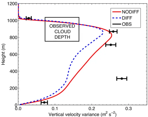
variance (w′_w′_{), or the vertical component of TKE, is a useful proxy for the strength}

of circulations within the STBL. For the highest and lowest of the five aircraft altitudes

(30 m and 1025 m), the DIFF and NODFF simulations exhibit very little difference. In

both cases, observed w′_w′ _{compares reasonably with modeled values. For the two}

flight legs at 710 and 870 m, observed values match well with NODIFF

(underesti-5

mated by 8 %), and are underestimated by 24 % and 12 %, respectively, by DIFF. For

the flight leg at 310 m altitude both simulations underestimatew′_w′_{by a factor of 2 (by}

54 % for DIFF and 46 % for NODIFF). NODIFF shows better agreement with observa-tions, since this particular configuration results in less entrainment of free tropospheric air and a smaller buoyancy sink of boundary layer TKE (Stevens et al., 2005). Thus

10

more energy is available to drive STBL circulations.

Investigation of profiles of buoyancy production of TKE and total water flux (Fig. 3)

reveal small differences between the two LES configurations. In the convective STBL,

buoyancy production of TKE is an important source term in the TKE budget (Nicholls, 1989). Radiative cooling at cloud top leads to negatively buoyant parcels that propagate

15

downward, driving STBL circulations. We find that buoyancy production of TKE within

cloud increases only slightly when sub-grid diffusion of scalars is neglected. This slight

increase is expected; less TKE is used to entrain potentially warmer air and mix it into the boundary layer (i.e. buoyancy destruction of TKE) when the entrainment rate is reduced. As we found in Fig. 2, the agreement between model and observations

20

appears reasonable in-cloud (overestimating by 7 % for DIFF and 25 % for NODIFF at 870 m) and poorer for the 300 m flight leg, underestimating by an order of magnitude in both cases. The observations in Figs. 2 and 3a suggest that parcels of air below cloud are more buoyant and lead to stronger updrafts and downdrafts in this region than what is simulated. Large-eddy simulation has been previously shown to underestimate

25

the strength of STBL circulations when compared to observations (e.g. Stevens et al., 2005).

(12)

ACPD

12, 27111–27172, 2012

Title Page

Tables Figures

◭ ◮

Back Close

Full Screen / Esc

Discussion

P

a

per

|

Dis

cussion

P

a

per

|

Discussion

P

a

per

|

Discussio

n

P

a

per

|

observed total water fluxes are subject to substantial uncertainties due to instrument precision. Both simulations exhibit a positive increase in total water flux with height and as the cloud is entered. Total water flux within the STBL is slightly larger for NODIFF because there is more total water within the STBL (Fig. 1b) and because circulations are slightly stronger (Fig. 2).

5

To determine how well the model can represent the observed variation in cloud LWC, we compared the probability distribution functions (PDF) of LWC as observed on the flight legs near cloud top and mid-cloud to the PDF of LWC in similar layers (Fig. 4).

The altitude of the Twin Otter varied by∼25 m and∼20 m on the two legs, respectively,

and we computed the PDF of LWC with LES output for the same thickness layers.

10

The PDFs from observations at cloud top exhibits a modal value between 0.42 and

0.43 g kg−1with a long tail towards smaller values of LWC (Fig. 4a). The wide

distribu-tion of LWC values observed is due to the Twin Otter traversing both diluted (entrain-ment of overlying dry air is substantial) and undiluted (entrain(entrain-ment of overlying dry air is small) cloud parcels. At mid-cloud the width of the PDF is narrower (Fig. 4d) because

15

at this height the cloud parcels are turbulently mixed and less entrainment of dry air

occurs at this height. The modal value between 0.16 and 0.17 g kg−1 is, as expected,

lower than at cloud top.

The modeled distributions of LWC at cloud top compare reasonably well with obser-vations. In general the PDFs from LES output (Fig. 4b, c, e, f) are less noisy because

20

there are an order of magnitude more sampling points in the LES than in the flight leg

(103 in the observations vs. 104 in the LES output). The similarity in PDF shape

be-tween the model output and observations is strong for DIFF (Fig. 4b). The modal value

at cloud top is between 0.35 and 0.36 g kg−1, slightly (16 %) lower than that observed.

At cloud top NODIFF (Fig. 4c) results in a modal value between 0.45 and 0.46 g kg−1

25

(neglecting zero LWC values), slightly higher (7 %) than that observed.

The two model predictions of the distribution of LWC mid-cloud both underestimate the modal value. For DIFF (Fig. 4e), the modal value mid-cloud (between 0.11 and

(13)

ACPD

12, 27111–27172, 2012

Title Page

Tables Figures

◭ ◮

Back Close

Full Screen / Esc

Discussion

P

a

per

|

Dis

cussion

P

a

per

|

Discussion

P

a

per

|

Discussio

n

P

a

per

|

and 0.16 g kg−1for NODIFF (Fig. 4f) is underestimated by 6 % compared to the

obser-vations. These differences in model output, paired with the errors at cloud top, suggest

di_ffering cloud thicknesses between DIFF and NODIFF. The NODIFF simulation

ex-hibits a thicker cloud layer than that of DIFF (265 m compared to 245 m).

It would be preferable to compare observed and simulated LWP. However, because

5

the aircraft sampling strategy focused mainly on horizontal legs it is not possible to generate statistically-significant observational estimates of LWP without assumption. If we assume an adiabatic profile of LWC in a 300 m thick cloud (as was observed), and set the cloud-top LWC value to the modal observed value, we derive an estimate for

LWP in the observed case of 65 g m−2. From LES time series output, LWPs averaged

10

over the simulated hour of observation for NODIFF and DIFF are 58.1 and 47.0 g m−2,

respectively. Thus both simulations appear to underestimate observed LWP (9.9 % and 27.1 %, respectively).

The performance of the two LESs in attaining reasonable agreement between model and observations for thermodynamic and flux profiles was comparable. Based on more

15

accurate representation of LWP and circulation strength with respect to observations

(shown in Fig. 2), we choose to use NODIFF, in which subgrid diffusion of scalars is

neglected, as the base case. Note that our choice does not imply that subgrid, turbulent

diffusion is negligible or irrelevant; we simply choose to neglect subgrid diffusion for

expediency and because of the better match between model output and observations.

20

5 Experimental design

5.1 Determining meteorological and aerosol perturbations

In creating the experimental simulations for the comparative study, we required that variations in meteorological context have three characteristics: (1) be constrained by observations, (2) be objectively computed, and (3) be determined consistently. In some

25

(14)

ACPD

12, 27111–27172, 2012

Title Page

Tables Figures

◭ ◮

Back Close

Full Screen / Esc

Discussion

P

a

per

|

Dis

cussion

P

a

per

|

Discussion

P

a

per

|

Discussio

n

P

a

per

|

maximize the possibility of finding a response. We prefer the perturbations to be more realistic so that the response of the stratocumulus cloud system to one perturbation can be reasonably compared with another.

To determine realistic perturbations in theqt and θjumps for stratocumulus clouds

in similar seasons and regions, we use the ERA-Interim dataset (Uppala et al., 2005,

5

2008). The ERA-Interim data, while spatially coarse as compared to available observa-tions, gives us a far larger temporal variation in meteorology than we would obtain from the observations taken from the Twin Otter during VOCALS (19 flights, 2 soundings taken per flight). Wyant et al. (2010) showed the ECMWF family of models reasonably matches satellite-observed stratocumulus cloud fractions for this region.

10

We first accumulated daily reanalysis data from the two nearest available

reanaly-sis data points to 20◦S, 72◦W, where the Twin Otter conducted all its flights (20.0◦S,

72.4◦W and 20.0◦S, 71.7◦W). The data is gridded at 2.5◦ by 2.5◦ latitude-longitude

resolution at six-hour intervals. From the surface (1000 mb) to an altitude of 700 mb, the vertical resolution is 25 mb. We used all days from September to November from

15

2001 to 2010 since stratocumulus is persistent during the austral spring in this region. We used 18Z data since this time most closely coincides with the observations.

Although stratocumulus is persistent in the observed region during the austral spring, the stratocumulus layer can be subjected to synoptic changes that influence its robust-ness (Rahn and Garreaud, 2010). To ensure that a stable stratocumulus layer existed

20

around 20◦S, 72.5◦W for all reanalysis data we excluded data on days when the low

cloud fraction was below 0.95 at either of the two reanalysis data points at either 12 and 18Z.

To ensure that the reanalysis data exhibit spatial homogeneity around 20◦S, 72.5◦W,

we also excluded days where the height of the inversion (height of the steepest

gra-25

dients in temperature and water vapor mixing ratio) did not coincide between the two grid points. Using these strict criteria, we were left with 60 data points from which to compute perturbations. From the accumulated data set we computed the standard

(15)

ACPD

12, 27111–27172, 2012

Title Page

Tables Figures

◭ ◮

Back Close

Full Screen / Esc

Discussion

P

a

per

|

Dis

cussion

P

a

per

|

Discussion

P

a

per

|

Discussio

n

P

a

per

|

the jump values within the ERA-Interim dataset do not coincide with the mean values in the model base case; it is the variation of these jumps within the ERA-Interim data that is of interest.

To modify theqt andθjumps above the boundary layer in the experimental

simula-tions, we altered the properties of the model free troposphere instead of the properties

5

of the model boundary layer. We first determined the height of the model boundary layer as the model layer for which the liquid water potential temperature gradient was maximized for each model column in the domain. We then modified the instantaneous

values ofqv orθfor all model layers above the boundary layer.

For the simulations where the θ jump was modified, we increased and decreased

10

the θ above the boundary layer by one standard deviation (UP THETA and DOWN

THETA,±1.3 K). Because the observed free troposphericq_v is low (below 1.0 g kg−1),

the two perturbations for theqtjump were both in the positive direction; by one standard

deviation (UP MOIST, +0.87 g kg−1) and by two standard deviations (UP 2XMOIST,

+1.74 g kg−1 ).

15

We would prefer that the perturbations in meteorological context and aerosol state originate from the same dataset and using the same methodology. Aerosol and cloud droplet data are not available in the ERA-Interim dataset, however, and we must use

a different methodology to get a “1-sigma” variation in aerosol state.

We chose to perturb only total aerosol concentrationNa, with no change in the mean

20

particle sizeDp(0.12 µm). The simulated change in cloud drop concentration correlates

strongly with the aerosol concentration perturbations. The initial mean values of model

NaandNd in the base case (Na=450 cm

−3

,Nd=425 cm

−3

) represent a strongly pol-luted stratocumulus case with substantial activation of aerosol. As a result, we elected not to impose an increase in aerosol concentration as a perturbation. Instead, we

main-25

tain the same aerosol size distribution shape and decrease the aerosol concentration by factors of 2 and 4 , thereby simulating moderately polluted (HALF ND) and fairly

clean (QUARTER ND) STBL cases, respectively. The lowest values ofNa=113 cm

−3 ,

Nd=106 cm

−3

(16)

ACPD

12, 27111–27172, 2012

Title Page

Tables Figures

◭ ◮

Back Close

Full Screen / Esc

Discussion

P

a

per

|

Dis

cussion

P

a

per

|

Discussion

P

a

per

|

Discussio

n

P

a

per

|

In order to span the full range of aerosol and cloud droplet concentrations observable

within stratocumulus, a lower-end value ofNd=50 cm

−3

is probably more appropriate,

while the upper rangeNd=425 cm

−3

is a reasonable upper value. Although we do not have decadal time series of aerosol data available for the region of interest, we note that

the Twin Otter observedNd to vary between 188 cm

−3

and 392 cm−3

during VOCALS

5

(Zheng et al., 2010). Thus the selectedNd range is probably larger than needed and

somewhat overestimates the variability in aerosol state in matching the 1-sigma vari-ability in meteorology. We keep this is mind when comparing cloud responses across meteorological and aerosol perturbations.

We also chose to test the response of stratocumulus to one hour temporal

dif-10

ferences in SW radiative heating. Aerosol-cloud interactions have been studied from polar-orbiting satellites (e.g. Nakajima et al., 1991; Painemal and Zuidema, 2010) but the time at which a satellite observes any given region varies by approximately one hour (the approximate return period). Thus, we seek to understand how such one-hour changes in SW heating might influence stratocumulus properties as observed

15

from space. Such results are also potentially relevant to aircraft campaigns, when the observational period can shift from day-to-day.

The aerosol and meteorological properties that are varied, the magnitude of these variations, and possible ways in which the cloud will respond to these variations, are summarized in Table 4. We focused on the response of stratocumulus to those

meteo-20

rological factors likely to modify STBL evolution on time scales less than a day.

5.2 Configuration of experimental simulations

By perturbing the base simulation with one perturbation at a time from Table 4 (two

different perturbations of one aerosol and each of three meteorological properties), we

created eight separate experimental simulations. The perturbations described in the

25

previous subsection were added at 09:30 UTC, two hours into the base LES, and the simulations were allowed to run for an additional six hours, to 15:30 UTC. Simulating

(17)

ACPD

12, 27111–27172, 2012

Title Page

Tables Figures

◭ ◮

Back Close

Full Screen / Esc

Discussion

P

a

per

|

Dis

cussion

P

a

per

|

Discussion

P

a

per

|

Discussio

n

P

a

per

|

through the observation period to near solar noon. For reference, Fig. 5 shows the temporal variation of solar insolation at TOA for the base simulation. This variation in solar insolation is shifted one hour back and one hour ahead in the SW forcing experiments.

As noted above, meteorological context and aerosol state are often correlated

(Bren-5

guier et al., 2003), but here we assume independence because attributing changes in

cloud properties∆c to changes in specific aerosol and meteorological factors will be

simpler if we only consider factors one at a time. Interactions between two or more

co-varying properties would make the attribution process more difficult. Examining

changes in cloud responses to co-varying aerosol and meteorological properties is

10

left to future study, possibly using the factorial method (Teller and Levin, 2008).

6 Results from experimental simulations

We first briefly describe the time evolution of the cloud layer in the model base case to provide some context for the discussion of the perturbation simulations. From

09:30 UTC to 15:30 UTC, the base case LWP decreases from 67 g m−2to 18 g m−2as

15

solar insolation increases. After 14:00 UTC the cloud layer has thinned such that it is optically thin in the longwave (LW) (Garrett and Zhao, 2006; Petters et al., 2012), and LW radiative cooling from the cloud top begins to decrease slightly with time. The boundary layer deepens over the six hours, reaching a nearly steady height at the end of simulation. This deepening indicates that entrainment of the overlying dry air

20

(18)

ACPD

12, 27111–27172, 2012

Title Page

Tables Figures

◭ ◮

Back Close

Full Screen / Esc

Discussion

P

a

per

|

Dis

cussion

P

a

per

|

Discussion

P

a

per

|

Discussio

n

P

a

per

|

6.1 Response to perturbations in potential temperature jump

Perturbations in the θ jump from the base case (labeled BASE) lead to changes in

entrainment rate that affect cloud LWP. Together Fig. 6a, f show that an increase in the

θabove the STBL leads to a higher LWP and vice versa (simulations UP THETA and

DOWN THETA, respectively).

5

As suggested by other studies (e.g. Lewellen and Lewellen, 1998; Sullivan et al.,

1998; Sun and Wang, 2008), an increase in theθ jump leads to stronger stability (i.e.

greater density contrast) across the interface, reducing the rate at which dry air from

above the cloud top entrains into the boundary layer. Also, because of the increase inθ

above the boundary layer, cloud integrated LW radiative cooling is reduced (Fig. 6c) and

10

hence there is less buoyant production of TKE within the cloud layer (Fig. 6e). Buoyant production is the primary source of TKE within the convective STBL, and a decrease in this quantity results in less TKE available to drive entrainment. Taken together, these two mechanisms lead to a slower increase in boundary layer height (Fig. 6b). Boundary layer height is directly related to entrainment rate because large-scale subsidence is

15

the same in all simulations (see Table 1).

The converse of these qualitative arguments applies when theθjump is decreased.

However, the cloud response is not identical in magnitude for the positive and negative

θjumps, i.e. the response is not symmetric.

As the sun rises toward mid-day and cloud integrated SW radiative heating increases

20

(Fig. 6d), LWP decreases in all three simulations. Shortwave radiative heating in-creases with LWP and explains in part why the LWP for the UP THETA simulation decreases more rapidly after 13:00 UTC as compared to the other two. Integrated LW cooling also decreases after 13:00 UTC in all three simulations as the cloud layer be-comes optically thin in that portion of the electromagnetic spectrum.

(19)

ACPD

12, 27111–27172, 2012

Title Page

Tables Figures

◭ ◮

Back Close

Full Screen / Esc

Discussion

P

a

per

|

Dis

cussion

P

a

per

|

Discussion

P

a

per

|

Discussio

n

P

a

per

|

6.2 Response to perturbations in moisture jump

For the base case, decreases in the magnitude of theqt jump(s) (i.e. moistening the

free troposphere) lead to increases in LWP (Fig. 7a, f). Like the STBL response to

changes in the θ jump, changes in LWP are related to changes in the entrainment

process and the magnitude of LW radiative cooling. For the same amount of entrained

5

overlying air into the STBL, increasingqvabove the boundary layer leads to less

evapo-ration of cloud and less associated evaporative cooling. This change in the entrainment

process partly explains both the increase in LWP with increasing free troposphericqt,

as well as the increase in latent heating at cloud top (Fig. 7d). Simultaneously, inte-grated LW radiative cooling decreases as there is more water vapor to emit LW

radia-10

tion to the top of the cloud (Fig. 7c).

As in Fig. 6, this decrease in integrated LW cooling (in conjunction with less cloud top evaporative cooling) leads to less buoyancy production of TKE (Fig. 7e) when the

magnitude of theqt jump decreases. Again, as this in-cloud buoyancy production

de-creases, we find a reduction in entrainment rate, which can be seen as a reduction in

15

boundary layer growth (Fig. 7b). This reduction in entrainment rate with increased free

troposphericqtalso leads to less evaporation of cloud. There is less mixing of relatively

dry overlying air into the cloud, and what mixing does occur brings in moister cloud-free air.

Different from the perturbations inθjump, one of the simulations, UP 2XMOIST, does

20

not appear to become optically thin in the LW spectrum near the end of simulation. In-tegrated LW radiative cooling decreases only slightly at the end of simulation, whereas for the other two (BASE and UP MOIST) LW cooling decreases more substantially (Fig. 7c). Furthermore, comparing Fig. 6a to Fig. 7a shows that the response of LWP

to the moisture jump perturbations is larger than the response toθjump perturbations.

25

This difference in LWP response has important bearing on the associated responses

(20)

ACPD

12, 27111–27172, 2012

Title Page

Tables Figures

◭ ◮

Back Close

Full Screen / Esc

Discussion

P

a

per

|

Dis

cussion

P

a

per

|

Discussion

P

a

per

|

Discussio

n

P

a

per

|

6.3 Response to perturbations in radiative heating

Displacing the time of sunrise one hour earlier (simulation RAD EARLY) leads to a de-crease in LWP, and delaying sunrise by one hour (simulation RAD LATE) leads to the opposite response (Fig. 8a). In general, SW heating decreases LWP by warming the cloud layer, and more SW heating integrated over simulation time further decreases

5

LWP (Fig. 8d).

Shortwave heating can also weaken circulations in the STBL through stabilizing the cloud layer with respect to the sub-cloud layer (e.g. Turton and Nicholls, 1987), and can lead to the cloud layer becoming somewhat decoupled from the subcloud layer and surface (e.g. Turton and Nicholls, 1987; Lu and Seinfeld, 2005; Sandu et al., 2008;

10

Petters et al., 2012). This decoupling can lead to further reductions in LWP because the cloud layer now receives less water vapor flux from below cloud. Profiles of vertical

velocity variance (w′_w′_{) for 12:30 to 13:30 UTC show that increases in total SW forcing}

over simulation time (RAD EARLY) lead to substantial reductions in circulation strength

(Fig. 8f). For RAD EARLY, w′_w′ _{exhibits a local minima in the STBL, indicating that}

15

some decoupling first occurs in that simulation.

Owing to the weakening of circulation strength with increases in SW forcing, we also find a reduction in entrainment rate (Fig. 8b). A reduction in the rate at which overlying dry air mixes into the boundary layer could lead to an increase in LWP. Liquid water path decreases instead, and thus the combination of SW warming and reduced water

20

vapor flux from the sub-cloud layer into the cloud more than offset the impact of this

decrease in entrainment rate.

The increase in total SW forcing over simulation time for RAD EARLY results in a thinner cloud layer with a lower cloud fraction at the end of simulation as compared to the model base case (Fig. 8e). Cloud fractions are defined as the ratio of model

25

columns with LWP<10 g m−2 to the total number of model columns. As the amount

(21)

ACPD

12, 27111–27172, 2012

Title Page

Tables Figures

◭ ◮

Back Close

Full Screen / Esc

Discussion

P

a

per

|

Dis

cussion

P

a

per

|

Discussion

P

a

per

|

Discussio

n

P

a

per

|

of simulation. These results suggest that modest (∼1 h) changes in the time of

ob-servation (e.g. by satellite or aircraft) can lead to substantial changes in the radiative properties of a stratocumulus layer. We discuss these changes in Sect. 7.

6.4 Response to perturbations in aerosol concentration

Previous studies have shown that perturbations inN_aand N_dcan lead to either cloud

5

thinning or thickening. When large scale forcings such as subsidence and SW forcing are held constant, changes in either the drizzle process (Albrecht, 1989; Jiang et al., 2002) or the entrainment process (Ackerman et al., 2004; Bretherton et al., 2007; Hill et al., 2009) can each play important roles in the STBL response. We found that, com-pared to our descriptions of cloud response to the meteorological perturbations,

ac-10

curate description of how perturbations toNa andNdimpact the simulations requires

more elaboration.

Relative to the base case, decreases inNaandNdlead to increases in LWP (Fig. 9a).

Increases in LWP with decreases in Na and Nd occur almost immediately after the

aerosol perturbations were introduced at 09:30 UTC. What is the mechanism

caus-15

ing the immediate divergence in model LWPs with changes inNa and Nd? Because

the thermodynamic profiles of all three simulations are identical immediately after the aerosol perturbations are introduced, it is unlikely that thermodynamics play a role in the immediate response (though feedbacks to the thermodynamic state could strongly

affect longer time-scale responses). Instead we look to immediate changes in

micro-20

physical processes when cloud droplet concentration is altered (Fig. 10).

Our simulations exhibit a weak drizzle process. Even when Nd is decreased to its

lowest value in QUARTER ND there is negligible sedimentation of cloud water below cloud base (not shown). Thus we look to potential changes in the entrainment process. When cloud droplet concentration is decreased evaporative cooling at cloud top is

ex-25

(22)

ACPD

12, 27111–27172, 2012

Title Page

Tables Figures

◭ ◮

Back Close

Full Screen / Esc

Discussion

P

a

per

|

Dis

cussion

P

a

per

|

Discussion

P

a

per

|

Discussio

n

P

a

per

|

Hill et al., 2009), and there are fewer droplets near the cloud top interface because larger droplets sediment faster (Bretherton et al., 2007; Hill et al., 2009).

As the evaporation rate near cloud top decreases, LWP would be expected to in-crease. We see that, for the first half hour after perturbations are induced, evaporative cooling (negative latent heating) at cloud top (associated with entrainment) does

de-5

crease with decreases in Na and Nd (Fig. 10a). Thus these changes in evaporation

at cloud top can be related to the increases in LWP seen in Fig. 9a immediately after 09:30 UTC.

Less evaporative cooling at cloud top also causes less buoyancy production of TKE

in that region (Fig. 10c), resulting in decreases inw′_w′_{near cloud top (Fig. 10b, around}

10

800 m altitude). Weaker turbulence leads to less vigorous entrainment, and thereby larger LWP can be maintained. As a whole this process is known as the

evaporation-entrainment effect (Hill et al., 2009). This effect could also play a role in the immediate

increases in LWP with decreasedNdat 09:30 UTC.

We note our model vertical resolution of 5 m is unable to explicitly resolve mixing

15

across the stratocumulus cloud top interface (Stevens et al., 2005). Even with subgrid

fluxes turned off, spurious diffusion of cloud droplets across the interface can occur

within LES, leading to an overestimation of entrainment efficiency (Bretherton et al.,

1999). We anticipate this overestimation to somewhat exaggerate the strength of cloud

top evaporation and its dependence onNaandNd.

20

We also find that, in response to the evaporation-entrainment effect, boundary layer

growth decreases with decreases inNd(Fig. 9b) as entrainment rate decreases. This

change in boundary layer growth plays an important role in the further evolution of these simulations. Before we elaborate further, we first consider the impacts of LW radiative cooling and SW radiative heating.

25

Figure 9c shows us that integrated LW cooling is similar across all three simulations

until about 13:30 UTC. After 13:30 UTC we see that LW cooling is dependent on Nd

due to variations in cloud thinning and reductions in cloud fraction withNd (Fig. 9e).

(23)

ACPD

12, 27111–27172, 2012

Title Page

Tables Figures

◭ ◮

Back Close

Full Screen / Esc

Discussion

P

a

per

|

Dis

cussion

P

a

per

|

Discussion

P

a

per

|

Discussio

n

P

a

per

|

fraction increases and individual cloudy model columns are more likely to be optically

thick in the LW. This change in LW cooling withNdcould help explain the slight increase

in differences in LWP across the three simulations after 13:30 UTC; more LW cooling

within the boundary layer can lead to cloud growth through a lowering of the lifting condensation level.

5

Decreases in Nd lead to more integrated SW heating (Fig. 9d). Because cloud

in-tegrated SW heating increases with increases in both LWP and Nd, it is clear that

the increase in LWP and consequent increase in cloud SW heating dominates the

ex-pected decrease in SW heating due to decreases inNd. If SW heating were to play

a primary role, we would expect LWP values across the simulations to become more

10

similar during the day because higher LWP values beget more heating and would lead to more cloud evaporation. Because we do not find this relationship between LWP and

Nd (Fig. 9a), we turn to the role of boundary layer growth and entrainment to explain

the simulated longer-term response to aerosol.

Averaged over the fourth hour of simulation after the perturbations were induced

15

(12:30 to 13:30 UTC),qvandθprofiles indicate that, asNddecreases, a cooler, moister

STBL results (Fig. 10d, e) that leads to more cloud growth. This cooler, moister STBL can be attributed to slower boundary layer growth and entrainment (Fig. 9b); more entrainment of warm, dry overlying air leads to a warmer, drier STBL. Note that Fig. 10d and e are qualitatively representative of adjacent hourly periods for these simulations.

20

Although the differences are small, we see near cloud top (900 m to 1000 m) for the

hour between 12:30 and 13:30 UTC that w′_w′ _{is smaller for the lower values of} _N

d (Fig. 10f). This relationship can again be associated with the evaporation-entrainment feedback, as we found near cloud top from 09:30 UTC to 09:45 UTC (Fig. 10b). This

relationship between circulation strength andNdnear cloud top is in contrast with the

25

more obvious increase ofw′_w′_{with decreases in}_N

dfor the bulk of the STBL. However,

(24)

ACPD

12, 27111–27172, 2012

Title Page

Tables Figures

◭ ◮

Back Close

Full Screen / Esc

Discussion

P

a

per

|

Dis

cussion

P

a

per

|

Discussion

P

a

per

|

Discussio

n

P

a

per

|

et al. (2003), Figs. 9 and 10 show that decreases in evaporative cooling and

entrain-ment rate with decreases inNaandNdresult in the increases of LWP found in this set

of simulations.

7 Computed responses in cloud properties

To objectively compare the impact of the perturbations in meteorological context∆m

5

and aerosol state ∆a on the model base case, we computed the response of three

cloud properties∆c(LWP,τand CRF) to these perturbations. We computed these

re-sponses from 5-min domain averaged cloud properties, averaged over one hour cen-tered on each of the last four hours of simulation (12:00, 13:00, 14:00 and 15:00 UTC). Because we have two separate perturbations (e.g. UP THETA and DOWN THETA)

10

for each of the four perturbed parameters, we computed two hourly-averaged cloud responses for each hour.

For all perturbation types, the two responses are reported by comparing cloud

prop-erties for (i) the simulations using themiddle (absolute) value ofθjump, qt jump, Na,

and SW forcing relative to the simulation usingsmallestvalue, and then (ii) by

compar-15

ing the simulations using thelargest perturbed parameter value relative to themiddle

value. See Table 5 for the exact choice of simulations used for each response calcula-tion.

Figures 11 to 14 show these computed responses. While the hour over which we average is the same for all responses, we slightly shift the results left or right at each

20

hour for clarity. As shown in Table 5, at each hour in Figs. 11 to 14 the point slightly shifted to the left is for the middle–smallest simulations, while the point shifted to the right is for the largest–middle simulations.

Although cloud responses to changes in SW forcing (simulations RAD EARLY and RAD LATE) are included in the Figs. 11 and 12, we discuss cloud responses to

25

these variations in a separate subsection (Sect. 7.2). Because solar insolation for

(25)

ACPD

12, 27111–27172, 2012

Title Page

Tables Figures

◭ ◮

Back Close

Full Screen / Esc

Discussion

P

a

per

|

Dis

cussion

P

a

per

|

Discussion

P

a

per

|

Discussio

n

P

a

per

|

simulations, we do not compute CRF responses to variations in SW forcing (i.e. in Fig. 13 and 14).

7.1 Responses to changes in jump properties compared to responses to

changes in droplet concentration

7.1.1 Liquid water path

5

Figure 11 shows the time evolution of responses of LWP. Averaged over the two

re-sponses at each hour and across all four hours, the LWP response to increases inNd

is the largest in magnitude (−13 g m−2), followed by the response to increases in theq_t

jump (−8 g m−2). The average LWP response to increases in theθjump is the smallest

at 5 g m−2.

10

For each perturbation, the LWP response varies with hour and, in some cases, at each hour between the two perturbations (e.g. UP THETA and DOWN THETA). The

LWP responses to increases in theθjump are all positive and vary the least over

sim-ulation time (between 2 and 7 g m−2). The LWP responses to increases in theqt jump

(decrease in free troposphericqtare all negative, varying between −5 and−12 g m

−2 .

15

Within each hourly average, the LWP response to changes inθ jump are fairly linear

(e.g. the response at each hour for UP THETA and DOWN THETA are similar). For

changes in theqtjump, the LWP response is fairly linear at 12:00 and 13:00 UTC and

less so at 14:00 and 15:00 UTC.

The LWP responses to increases in Nd are all negative and vary between −6 and

20

−23 g m−2. For all four hours we find a non-linear LWP response to these increases in

Nd. The first increase fromNd=106 cm

−3

toNd=213 cm

−3

yields the larger response

in LWP, and is associated with non-linear changes in entrainment rate withNd(Fig. 9b).

This non-linearity increases with time.

Because of the substantial decrease in LWP during the day, relative LWP responses

25

(26)

ACPD

12, 27111–27172, 2012

Title Page

Tables Figures

◭ ◮

Back Close

Full Screen / Esc

Discussion

P

a

per

|

Dis

cussion

P

a

per

|

Discussion

P

a

per

|

Discussio

n

P

a

per

|

relative LWP responses to increases inNdvary from−10 % at 12:00 UTC to−94 % at

15:00 UTC, when the cloud layer is thinnest.

7.1.2 Optical depth

We found LWP responses to changes in meteorological perturbations (∆m) to be of

the same magnitude, or smaller, than LWP responses to aerosol perturbations (∆a)

5

(Fig. 11). However, LWP responses to these perturbations can not be directly translated

into radiative responses. In general bulk optical depthτis proportional to LWP,Ndand

the dispersion of the cloud drop size distribution, represented by k (Brenguier et al.,

2011):

τ∼(kN_d)1/3LWP5/6. (1)

10

We computedτfor the SW portion of the spectrum using:

τ=

z_t Z

z_b r_u Z

r_l

2πr2n(r)drdz, (2)

wherezt and zbare the heights of the cloud top and cloud base, respectively, ru and

rl are the radius size range of the drop size distribution and n(r) is the number of

drops betweenr and r+dr (Seinfeld and Pandis, 1998). The extinction efficiency is

15

assumed to be 2. Using output of 5-min averaged cloud droplet size distribution data, we integrated the model drop size distribution first over the 25 bins in the microphysical

model and then over the total depth of the cloud layer. For the base case, changes inτ

with time follows the same trend as LWP with time (compare the black lines on Fig. 11 and Fig. 12), as expected from Eq. (1).

20

Optical depth responses to perturbations in the two jump properties are proportional

to LWP responses (Fig. 12). For increases inqt jump strength, hourly-averaged values