www.atmos-chem-phys.net/15/2247/2015/ doi:10.5194/acp-15-2247-2015
© Author(s) 2015. CC Attribution 3.0 License.
Aerosol size distribution and radiative forcing response to
anthropogenically driven historical changes in biogenic secondary
organic aerosol formation
S. D. D’Andrea1, J. C. Acosta Navarro2, S. C. Farina1, C. E. Scott3, A. Rap3, D. K. Farmer4, D. V. Spracklen3, I. Riipinen2,5, and J. R. Pierce1,6
1Department of Atmospheric Science, Colorado State University, Fort Collins, CO, USA
2Department of Applied Environmental Science and Bert Bolin Centre for Climate Research, Stockholm University,
Stockholm, Sweden
3School of Earth and Environment, University of Leeds, Leeds, UK
4Department of Chemistry, Colorado State University, Fort Collins, CO, USA
5Center for Atmospheric Particle Studies, Carnegie Mellon University, Pittsburgh, PA, USA 6Department of Physics and Atmospheric Science, Dalhousie University, Halifax, NS, Canada
Correspondence to:S. D. D’Andrea ([email protected])
Received: 30 September 2014 – Published in Atmos. Chem. Phys. Discuss.: 20 October 2014 Revised: 29 January 2015 – Accepted: 5 February 2015 – Published: 2 March 2015
Abstract. Emissions of biogenic volatile organic com-pounds (BVOCs) have changed in the past millennium due to changes in land use, temperature, and CO2
concentra-tions. Recent reconstructions of BVOC emissions have pre-dicted that global isoprene emissions have decreased, while monoterpene and sesquiterpene emissions have increased; however, all three show regional variability due to compe-tition between the various influencing factors.
In this work, we use two modeled estimates of BVOC emissions from the years 1000 to 2000 to test the effect of anthropogenic changes to BVOC emissions on secondary or-ganic aerosol (SOA) formation, global aerosol size distribu-tions, and radiative effects using the GEOS-Chem-TOMAS (Goddard Earth Observing System; TwO-Moment Aerosol Sectional) global aerosol microphysics model. With anthro-pogenic emissions (e.g., SO2, NOx, primary aerosols) turned
off and BVOC emissions changed from year 1000 to year 2000 values, decreases in the number concentration of parti-cles of sizeDp> 80 nm (N80) of > 25 % in year 2000 relative
to year 1000 were predicted in regions with extensive land-use changes since year 1000 which led to regional increases in the combined aerosol radiative effect (direct and indirect) of > 0.5 W m−2 in these regions. We test the sensitivity of our results to BVOC emissions inventory, SOA yields, and
the presence of anthropogenic emissions; however, the quali-tative response of the model to historic BVOC changes re-mains the same in all cases. Accounting for these uncer-tainties, we estimate millennial changes in BVOC emissions cause a global mean direct effect of between +0.022 and +0.163 W m−2and the global mean cloud-albedo aerosol in-direct effect of between −0.008 and −0.056 W m−2. This change in aerosols, and the associated radiative forcing, could be a largely overlooked and important anthropogenic aerosol effect on regional climates.
1 Introduction
Biogenic volatile organic compounds (BVOCs) play an im-portant role in tropospheric chemistry and pollution by re-acting with the hydroxyl radical (OH), nitrate radical (NO3),
and ozone (O3)(Chung and Seinfeld, 2002). BVOCs are also
important precursors for O3 (Chameides et al., 1998) and
2013; Acosta Navarro et al., 2014). Changes in land use, tem-perature, and carbon dioxide (CO2)concentrations have all
had significant impacts on the emissions of BVOCs. Acosta Navarro et al. (2014) predicted that globally aver-aged isoprene emissions have decreased over the past mil-lennium mainly due to land-use changes, which involved the conversion of high-isoprene-emitting natural shrubs and broadleaf trees to low-emitting crop and grazing land. They also predicted that globally averaged monoterpene and sesquiterpene emissions have increased over the past mil-lennium due mainly to global increases in temperature (the monoterpene- and sesquiterpene-emitting vegetation has not decreased from land-use changes to the same degree as the isoprene-emitting vegetation). However, all three BVOC classes show both increases and decreases in various regions due to competing factors such as land-use change, increases in CO2 concentrations, and temperature change. The most
dominant cause of BVOC emission changes has been from anthropogenic factors (e.g., change in land cover and CO2
effects), where land-use change has had the most dramatic impact by decreasing the isoprene emissions. These changes in BVOC emissions can have important implications on the formation rate of low-volatility SOA, which is essential for particle growth to sizes large enough to affect climate (Ri-ipinen et al., 2011, 2012; Paasonen et al., 2013; Liao et al., 2014).
The Earth’s radiation balance is directly affected by aerosol particles by absorption and scattering of solar ra-diation (Rosenfeld et al., 2008; Clement et al., 2009) as well as indirectly affected by aerosols by alteration of cloud properties and lifetimes (Charlson et al., 1992). The uncer-tainty associated with aerosol radiative forcing, particularly the aerosol indirect effect, is a large source of uncertainty in global climate models (Forster et al., 2007). Recent stud-ies suggest that this uncertainty is largely due to incom-plete knowledge on different natural contributions to atmo-spheric aerosol loadings (Carslaw et al., 2013). The influence of aerosols on cloud droplet number concentration (CDNC) is driven by the number concentration of cloud condensa-tion nuclei (CCN), the particles on which cloud droplets form. The number concentration of CCN is highly dependent on the aerosol size distribution (Dusek et al., 2006; McFig-gans et al., 2006; Petters and Kreidenweis, 2007; Pierce and Adams, 2007); therefore, the size-dependent number of all sizes of particles must be accurately represented to simulate CCN number concentrations correctly.
The two sources of aerosol number concentrations in the atmosphere are primary emissions (Putaud et al., 2004; Stanier et al., 2004) and the formation of new particles (diam-eter ∼1 nm) via nucleation (Kulmala et al., 2004). In order for freshly nucleated particles or emitted nanoparticles with diameters less than CCN sizes (30–100 nm) to influence at-mospheric CCN number concentrations, they must undergo condensational growth (Pierce and Adams, 2007; Vehkamäki and Riipinen, 2012). However, the survival probability of
nanoparticles depends on the competition between condensa-tional growth and coagulacondensa-tional scavenging with pre-existing aerosol (Kerminen and Kulmala, 2002; Pierce and Adams, 2007; Kuang et al., 2009; Westervelt et al., 2013).
In the following section, we summarize the global millen-nial changes in biogenic emissions from Acosta Navarro et al. (2014). Section 3 describes the model used in this study and the methods used for formation of SOA from the bio-genic terpenoid emissions. Section 4 describes the results, highlighting the global changes in particle size distributions due to the millennial changes in BVOC emissions and the climatic implications associated with these changes.
2 Overview of predicted BVOC emissions changes Acosta Navarro et al. (2014) used the Model of Emissions and Gases and Aerosols from Nature (MEGAN) (Guenther et al., 2006) and the Lund–Potsdam–Jena General Ecosys-tem Generator (LPJ-GUESS) (Smith et al., 2001; Sitch et al., 2003) to reconstruct BVOC emissions from the year 1000 to the year 2000. This is described in detail by Acosta Navarro et al. (2014), but will be summarized here. For this study, we refer to the decadal-averaged BVOC emissions us-ing MEGAN from 1000–1010 and from 1980–1990 as years 1000 and 2000, respectively, for simplicity. We refer to the annual-averaged BVOC emissions using LPJ-GUESS from years 1000 and 2000 as years 1000 and 2000, respectively. Because our LPJ-GUESS emissions are from one single year at 1000 and 2000, these data may be susceptible to some re-gional biases due to not capturing interannual variability.
The MEGAN reconstruction includes all three BVOC classes, whereas the LPJ-GUESS reconstruction includes only isoprene and monoterpenes. MEGAN and LPJ-GUESS were run in a series of simulations testing sensitivities to vari-ables (such as plant functional type, leaf area index, soil wa-ter content, annual CO2concentrations, land-use cover, and
anthropogenic vegetation types such as crops and pastures), and millennial terpenoid BVOC emission inventories were created (Acosta Navarro et al., 2014). The main driving fac-tors behind the changes are not always the same (for details see Acosta Navarro et al., 2014).
The terpenoid BVOC emissions in Acosta Navarro et al. (2014) are sensitive to variations in meteorological con-ditions and land-use changes, but are also sensitive to the empirical standard emission factors used in the developing of the inventory. Plant emission factors of the three BVOCs were averaged over wide plant families in order to make the model computationally feasible. Therefore, the changes in isoprene, monoterpenes, and sesquiterpenes in the recon-struction are indicators of the response of the three BVOCs to external stresses and land-use change, rather than exact sion estimates. Also, changing the resolution of the emis-sions inventory from the original resolution to a coarser res-olution may inherently have uncertainties.
Isoprene has the highest predicted emission rates of the BVOCs investigated in this study with emis-sions averaged over the time period 1000–1990 greater than 50 mg m−2day−1 using MEGAN and greater than
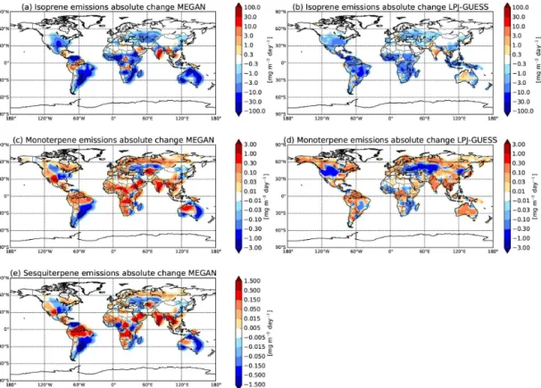
30 mg m−2day−1 averaged over the period 1000–2000 us-ing LPJ-GUESS over tropical rainforests (Acosta Navarro et al., 2014). These emissions are roughly a factor of 100 lower over mid-latitude forests. Isoprene emissions are dominant in tropical and sub-tropical regions but much lower in boreal regions. Predicted absolute changes in the spatial distribu-tion of mean isoprene emissions from 1000 to 2000 using MEGAN and LPJ-GUESS are shown in Fig. 1a and b, re-spectively. Globally averaged, predicted isoprene emissions over this period decrease by 21 % in MEGAN and 23 % in LPJ-GUESS, and these decreases are due predominantly to cropland expansion and CO2 concentration effects (Acosta
Navarro et al., 2014). The changes in land-use due to natu-ral high isoprene-emitting broadleaf trees and shrubs being converted to low-isoprene-emitting crops and grasses, such as in plantations and pastures, have directly decreased iso-prene emissions regionally in both reconstructions. The trop-ical and sub-troptrop-ical regions with high isoprene emissions are the regions with the largest absolute changes in emis-sions over this time period. There is some evidence for de-creases in isoprene emissions with increasing CO2
concen-trations, although the related mechanisms are not well un-derstood (Peñuelas and Staudt, 2010). The effects are in-cluded in MEGAN and LPJ-GUESS, so both of the mod-els applied by Acosta Navarro et al. (2014) suggest that in-creasing CO2concentrations in the present-day atmosphere
also contribute to the decrease in isoprene emissions. How-ever, isoprene emissions in some regions where the natural vegetation has remained unaltered or increased over the past millennium have increased by greater than 50 % in both re-constructions due to the increase in surface air temperature (Acosta Navarro et al., 2014).
Along with changes in isoprene emissions over the past millennium, predicted monoterpene emissions also change, but due to different environmental and anthropogenic influ-ences. Mean predicted emissions of monoterpenes over the period 1000–2000 are roughly an order of magnitude lower than predicted isoprene emissions, but are still greater than 5 mg m−2day−1and 0.8 mg m−2day−1in tropical and sub-tropical forests in the MEGAN and LPJ-GUESS reconstruc-tions, respectively (Acosta Navarro et al., 2014). Predicted absolute changes in the spatial distribution of mean monoter-pene emissions from 1000 to 2000 using MEGAN and LPJ-GUESS are shown in Fig. 1c and d, respectively. Globally av-eraged, predicted monoterpene emissions over this period in-crease by 3 % in MEGAN and 0 % in LPJ-GUESS. However, in many regions there is an increase in predicted monoter-pene emissions of approximately 0.5 mg m−2day−1. These
Figure 1.Absolute change in(a)isoprene,(c)monoterpene, and(e)sesquiterpene emissions between the years 1000–1010 and 1980–1990 in mg m−2day−1from the MEGAN terpenoid reconstruction, and absolute change in(b)isoprene, and(d)monoterpene emissions between
the years 1000 and 2000 in mg m−2day−1from the LPJ-GUESS terpenoid reconstruction (Acosta Navarro et al., 2014). Note the change of
scale between panels. An increase in emissions is represented in red, and a decrease in isoprene emissions in blue.
It is worthwhile to note that the effect of CO2concentrations
on monoterpene emissions is still under debate, and was not included in the simulations by Acosta Navarro et al. (2014) applied here. We also note that the temperature response of BVOC emissions used to predict long-term changes is de-rived from short-term measurements, and may not accurately reflect the adaptive behavior of plants grown under changing environmental conditions.
Similar to changes in predicted monoterpene emissions over the past millennium, sesquiterpene emissions have also been predicted to increase regionally although remaining ap-proximately constant globally. Mean predicted emissions of sesquiterpenes over the period 1000–2000 are spatially dis-tributed similar to that of monoterpene emissions and are an order of magnitude lower than predicted monoterpene emis-sions, and 2 orders of magnitude lower than predicted iso-prene emissions. Figure 1e shows the absolute change in predicted sesquiterpene emissions from 1000 to 2000 using MEGAN. Following the same trend as predicted monoter-penes, the globally averaged change in predicted sesquiter-pene emissions over this period increase by approximately 1 %. The causes of the changes in predicted sesquiterpene emissions are analogous to the changes in predicted monoter-pene emissions. The changes are predominantly due to
de-velopment of agriculture in regions where sesquiterpene-emitting vegetation was previously limited (Acosta Navarro et al., 2014).
3 Methods
We use a global chemical transport model with online aerosol microphysics to test the sensitivity of the simulated aerosol size distributions to changes in BVOC emissions from the years 1000 to 2000, and calculate the associated radiative forcing.
3.1 GEOS-Chem-TOMAS model description
We use the global chemical-transport model, GEOS-Chem (Goddard Earth Observing System) (http://www.geos-chem. org), combined with the online aerosol microphysics module, TOMAS (TwO-Moment Aerosol Sectional; GEOS-Chem-TOMAS) to test the sensitivity of global aerosol size distribu-tions to changes in BVOC emissions. GEOS-Chem-TOMAS in this study uses GEOS-Chem v9.01.02 with 4◦
simulates the aerosol size distribution using 15 size sections ranging from 3 nm to 10 µm (Lee and Adams, 2011). Nucle-ation rates in all simulNucle-ations were predicted by ternary ho-mogeneous nucleation of sulfuric acid, ammonia, and wa-ter based on the paramewa-terization of Napari et al. (2002) scaled globally by a constant factor of 10−5which has been shown to predict nucleation rates closer to measurements than other commonly used nucleation schemes (Jung et al., 2010; Westervelt et al., 2013). All emissions except terpenoid biogenic emissions (monoterpenes, isoprene, and sesquiter-penes) in GEOS-Chem are described in van Donkelaar et al. (2008). The three dominant BVOC classes (monoter-penes, isoprene, and sesquiterpenes) are included in GEOS-Chem using modeled reconstructions as provided by Acosta Navarro et al. (2014). The emissions from Acosta Navarro et al. (2014) override biogenic emissions previously input from a different version of MEGAN (Guenther et al., 2006) in the standard version of GEOS-Chem for SOA production only and do not influence the gas-phase chemistry in GEOS-Chem-TOMAS. We do not consider this feedback; however, we will discuss the implications in Sect. 4.4.
Traditionally, SOA in GEOS-Chem-TOMAS is formed only from terrestrial biogenic sources, with the biogenic source being a fixed yield of 10 % of the monoterpene emis-sions. However, isoprene and sesquiterpenes also serve as SOA precursors (Hoffmann et al., 1997; Griffin et al., 1999; Kroll et al., 2006). In this study, we form SOA from iso-prene, monoterpenes, and sesquiterpenes with fixed yields of 3, 10, and 20 %, respectively, based on estimations summa-rized in Pye et al. (2010). Dynamic SOA yields through parti-tioning theory are computationally expensive to couple with aerosol microphysics schemes, and they tend to underpre-dict ultrafine particle growth when lab-based volatility dis-tributions are used (Pierce et al., 2011), and thus are not used here. However, we test the sensitivity to these yields. The yields used in this study are on the low end of mean yield estimates; however, we test the sensitivity of SOA for-mation and CCN number concentrations to upper bounds on these yields (10, 20, and 40 %, respectively) (Pye et al., 2010) (see Table 1 for total biogenic SOA formation rates for each simulation). Biogenic SOA formation, particularly from isoprene, has been shown in chamber studies and ambi-ent measuremambi-ents to have dependencies on NOx
concentra-tions (NOx=NO+NO2)(Kroll et al., 2006; Kroll and
Sein-feld, 2008; Carlton et al., 2009; Xu et al., 2014). SOA yield from isoprene oxidation can reach in excess of 4 % under low-NOx conditions (Kroll et al., 2006) at atmospherically
relevant organic mass concentrations (Carlton et al., 2009). Kroll et al. (2006) also found in chamber studies that SOA yields from isoprene oxidation can reach in excess of 5 % at NOx concentrations of approximately 100 ppb. Over the
past millenium, there have been increases in agriculture, an-thropogenic biomass burning, and industrial activity leading to enhanced NOxemissions (Benkovitz et al., 1996), which
potentially impact SOA yields. More sophisticated SOA
for-mation mechanisms that account for NOx-dependent yields
might improve model representation; however, maximum NOx concentrations in GEOS-Chem-TOMAS are
approxi-mately an order of magnitude lower than the concentrations used in the chamber study by Kroll et al. (2006), Lamsal et al. (2008) and therefore fall well below NOxconcentrations
high enough to significantly alter SOA formation rates. We note that while high absolute concentrations of any species may call into question the atmospheric relevance of cham-ber experiments, the NO:HO2ratio within a chamber is an equally critical parameter for describing the chemical regime of SOA formation. Therefore, for this study, biogenic SOA in GEOS-Chem-TOMAS is formed via fixed yields of isoprene, monoterpenes, and sesquiterpenes, and has no dependency on NOxconcentrations. The change in emissions of isoprene,
monoterpenes, and sesquiterpenes from the MEGAN and LPJ-GUESS reconstructions solely affects SOA formation, and does not influence the oxidation fields in GEOS-Chem-TOMAS. Therefore, there may be missing feedback mecha-nisms on key atmospheric oxidants.
In this study, particles are assumed to undergo kinetic, gas-phase-diffusion-limited growth with condensation of SOA proportional to the Fuchs-corrected aerosol surface area. This assumption was found to best reproduce aerosol size distribu-tion in two recent studies (Riipinen et al., 2011; D’Andrea et al., 2013). This kinetic condensation of SOA assumes that the SOA is non-volatile (or similar to low-volatility SOA with average saturation vapor pressure,C*, of less than
approxi-mately 10−3µg m−3)(Pierce et al., 2011, Ehn et al., 2014). Also, as described in D’Andrea et al. (2013), an additional 100 Tg yr−1 of SOA correlated with anthropogenic carbon monoxide emissions is required to match present-day mea-surements. D’Andrea et al. (2013) evaluates GEOS-Chem-TOMAS particle number concentrations against measure-ments and shows that including the extra SOA yields im-proved number predictions for a wide range of particle sizes. The sensitivity of this additional source of SOA is also inves-tigated in this study.
We test the sensitivity of predicted size distributions to anthropogenically driven changes in BVOC emissions in GEOS-Chem-TOMAS using 12 simulations. Table 1 shows the assumptions in these 12 simulations. All simulations were run using 2005 meteorology with 3 months of spin-up from a pre-spun-up restart file.
Table 1. Summary of the GEOS-Chem-TOMAS simulations performed in this study. Biogenic emissions for year 1000 and 2000 using MEGAN are decadal-averaged emissions for 1000–1010 and 1980–1990, respectively, whereas LPJ-GUESS biogenic emissions are annual-averaged for the years 1000 and 2000. Standard SOA yields are 3, 10, and 20 % for isoprene, monoterpenes, and sesquiterpenes, respectively, and upper-bound SOA yields are 10, 20, and 40 % for isoprene, monoterpenes, and sesquiterpenes, respectively. In the simulation naming scheme, “BE” refers to biogenic emissions, “1” refers to year 1000, “2” refers to year 2000, “O” refers to off, “meg” refers to MEGAN BVOC emissions, “LPJ” refers to LPJ-GUESS BVOC emissions, “up” refers to upper-bound SOA yields, and “XSOA” refers to the inclusion of the additional 100 Tg (SOA) yr−1.
Simulation Biogenic Anthropogenic MEGAN LPJ- Standard Upper Additional Total
name emissions emissions Acosta GUESS SOA yield bound 100 Tg biogenic
Navarro Acosta SOA yield (SOA) yr−1 SOA
et al. Navarro D’Andrea formation (Tg yr−1)
(2014) et al. et al. rates
(2014) (2013)
BE1.AE2.meg 1000 YES YES NO YES NO NO 35.96
BE1.AEO.meg 1000 NO YES NO YES NO NO 35.96
BE2.AE2.meg 2000 YES YES NO YES NO NO 41.44
BE2.AEO.meg 2000 NO YES NO YES NO NO 41.44
BE1.AEO.LPJ 1000 NO NO YES YES NO NO 13.63
BE2.AEO.LPJ 2000 NO NO YES YES NO NO 16.81
BE1.AE2.up 1000 YES YES NO NO YES NO 100.30
BE1.AEO.up 1000 NO YES NO NO YES NO 100.30
BE2.AE2.up 2000 YES YES NO NO YES NO 118.92
BE2.AEO.up 2000 NO YES NO NO YES NO 118.92
BE1.XSOA 1000 YES YES NO YES NO YES 135.96
BE2.XSOA 2000 YES YES NO YES NO YES 141.44
with these changes in BVOC emissions. For gas-phase chem-istry, emissions of BVOCs are from online MEGAN for 2005 (Wainwright et al., 2012). Using the AE2 and AEO simu-lations, we can see if the sensitivity of aerosols and radia-tive forcing to changes in BVOC emissions is strongly sensi-tive to the presence of anthropogenic aerosols. First, we as-sume present-day anthropogenic emissions and have simul-taneous monthly mean BVOC emissions from MEGAN for the year 1000 (BE1.AE2.meg) and another simulation for the year 2000 also using MEGAN (BE2.AE2.meg) (the jus-tification for these time periods is explained in Sect. 2.3). This method isolates the change in BVOCs and the effect on aerosol size distributions under fixed anthropogenic sions. We also test the sensitivity to changes in BVOC emis-sions over the same periods with no anthropogenic emisemis-sions to simulate a pre-industrial anthropogenic environment us-ing MEGAN (BE1.AEO.meg and BE2.AEO.meg) and LPJ-GUESS (BE1.AEO.LPJ and BE2.AEO.LPJ). Using these simulations, we also test the sensitivity of predicted size distributions to changes in anthropogenic emissions under present-day BVOC emissions from MEGAN by comparing simulations (BE2.AEO.meg and BE2.AE2.meg). Thus, we estimate the effects of changing biogenic emissions in sets of simulations where the anthropogenic emissions are either on or off. While neither of these comparisons is realistic (anthro-pogenic emissions changed as the biogenic emissions were changing), it allows us to bound the impact of anthropogenic
emissions on the partial derivative with respect to changing biogenic emissions.
We also test the model sensitivity to changes in SOA yields (as described previously) over the same periods by re-peating the four simulations using MEGAN (BE1.AE2.meg, BE1.AEO.meg, BE2.AE2.meg, and BE2.AEO.meg) with upper bounds on the SOA yields (10, 20, and 40 % of isoprene, monoterpenes, and sesquiterpenes, respectively) (BE1.AE2.up, BE1.AEO.up, BE2.AE2.up, BE2.AEO.up). Finally, we investigate the sensitivity to the inclusion of an additional 100 Tg yr−1of anthropogenically enhanced SOA
(as described previously) in the simulations with present-day anthropogenic emissions using MEGAN biogenic emis-sions for year 1000 and year 2000 conditions (BE1.XSOA, BE2.XSOA). We note that the predicted size distributions and uncertainty ranges in this paper are sensitive to the nucle-ation scheme, anthropogenic emissions fluxes, and emissions size (e.g., Pierce and Adams, 2009), but here we explore the modeled partial derivatives to changes in BVOC emissions only.
3.2 Aerosol direct effect and the cloud-albedo aerosol indirect effect
which has been used previously in other aerosol micro-physics studies (Spracklen et al., 2011; Rap et al. 2013; Pierce et al. 2013; Scott et al. 2014). The ES radiative trans-fer model uses monthly mean cloud climatology and surface albedo, from the International Satellite Cloud Climatology Project (ISCCP) (Rossow and Schiffer, 1999), for the year 2000. Note that the land-use changes that lead to the changes in BVOC emissions explored in this paper may also lead to surface albedo and/or cloud changes; however, we do not ex-plore these changes in this paper.
To investigate the changes in DRE, an offline version of the RADAER module from the Hadley Centre Global Envi-ronment Model (Bellouin et al., 2013) was adapted to calcu-late aerosol optical parameters from GEOS-Chem-TOMAS output. The refractive index for each size section is calculated as the volume-weighted mean refractive index of the compo-nents (given at 500 nm in Table A1 of Bellouin et al., 2011), including water. Water uptake is tracked explicitly in GEOS-Chem-TOMAS by using ISSOROPIA (Nenes et al., 1998). For computational efficiency, the optical properties (dimen-sionless asymmetry parameter, and scattering and absorption coefficients, in m2kg−1)are then obtained from look-up ta-bles of all realistic combinations of refractive index and Mie parameter (particle radius normalized to wavelength), as de-scribed by Bellouin et al. (2013). These aerosol optical prop-erties were then included in monthly climatologies when run-ning the offline ES radiative transfer model.
The cloud-albedo AIE is calculated by perturbing the ef-fective radii of cloud droplets in the ES radiative transfer model. A control cloud droplet effective radius (re1)of 10 µm
is assumed uniformly, to maintain consistency with the IS-CCP derivation of liquid water path, and for each experiment a perturbed field of effective radii (re2)for low- and mid-level
(below 600 hPa) water clouds are calculated as in Eq. (1) us-ing the control (CDNC1)and perturbed (CDNC2)fields of
cloud droplet number concentration for each month.
re2=re1×
CDNC
1
CDNC2 1/3
(1)
We calculate monthly mean CDNC using the aerosol size dis-tributions predicted by GEOS-Chem-TOMAS and a mecha-nistic parameterization of cloud drop formation from Nenes and Seinfeld (2003), for a globally uniform updraft velocity of 0.2 m s−1. The assumption of a globally uniform updraft velocity is in itself a simplification and the AIE we calculate will be sensitive to the value used. Spracklen et al. (2011) and Pierce et al. (2013) found that assuming a base value of 0.2 m s−1gave an AIE close to the mean AIE obtained when
the globally uniform updraft velocity was varied between 0.1 and 0.5 m s−1. The cloud-albedo AIE is then calculated by comparing the perturbed (using re2) net radiative fluxes at
the top of the atmosphere to a control simulation (usingre1).
The DRE and cloud-albedo AIE are approximately addi-tive, but to give a combined aerosol radiative effect, one must
account for spatial overlap; therefore, a combined aerosol ra-diative effect is calculated by perturbing the cloud droplet ef-fective radii and aerosol climatologies at the same time in the ES radiative transfer model, and comparing the net radiative fluxes to a control simulation in which neither is perturbed.
4 Results
4.1 Changes to SOA formation rates
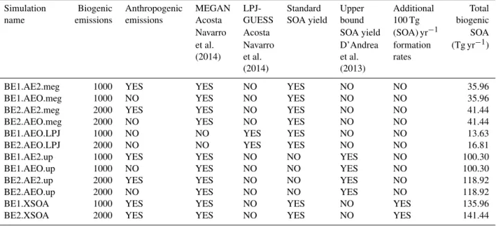
Figure 2a and b show the mean millennial fixed-yield SOA formation from MEGAN BVOC emissions (monoter-penes, isoprene, and sesquiterpenes) and LPJ-GUESS BVOC emissions (monoterpenes and isoprene), respectively, in mg m−2day−1over the years 1000–2000 and the base SOA yield assumptions. Figure 2c and e show the absolute and relative change in fixed-yield SOA formation from the same MEGAN BVOC emissions between 1000 and 2000 (year 2000–year 1000), respectively. Figures 2d and f show the absolute and relative change in fixed-yield SOA formation from the same LPJ-GUESS BVOC emissions between 1000 and 2000 (year 2000–year 1000), respectively. An increase in SOA formation with time is represented in red, and a de-crease in SOA formation in blue. Globally, the mean SOA formation from the MEGAN BVOC emissions decreases by 13.2, and decreases by 18.9 % from the LPJ-GUESS BVOC emissions. Regions such as central North America, eastern Australia, and southern South America show sig-nificant decreases, exceeding 75 % in SOA formation from the MEGAN BVOC emissions. There are also regions such as India, and southeast Asia with increases of greater than 50 % in SOA formation from the MEGAN BVOC emissions. These changes in emissions are largely due to millennial an-thropogenic influences on BVOC emissions through land-use changes. In Fig. 2e, there are regions with large per-cent increases or decreases in SOA formation, such as west-ern North America and northwest-ern Asia; however, the abso-lute change is negligible in these regions due to very low emissions. SOA formation from LPJ-GUESS BVOC emis-sions generally exhibits the same spatial pattern as MEGAN emissions. Where there are significant decreases/increases in BVOC emissions from 1000 to 2000, there are corresponding decreases/increases in SOA formation. Decreases/increases in SOA formation exceeding 50 % would significantly de-crease/increase the amount of low-volatility condensable or-ganic material available to grow nanoparticles in the atmo-sphere. Therefore, changes in SOA formation of this magni-tude could have an important anthropogenic aerosol effect on regional climates.
emis-Figure 2.Mean millennial fixed-yield biogenic SOA formation from(a)MEGAN emissions and(b)LPJ-GUESS emissions between the periods 1000–2000 in mg m−2day−1. Absolute change in fixed-yield biogenic SOA formation from averaged(c)MEGAN BVOC emissions
(monoterpenes, isoprene, and sesquiterpenes) and(d)LPJ-GUESS BVOC emissions (monoterpenes and isoprene) between 1000 and 2000 in mg m−2day−1. Relative change in fixed-yield biogenic SOA formation from averaged
(e)MEGAN BVOC emissions (monoterpenes, isoprene, and sesquiterpenes) and(f)LPJ-GUESS BVOC emissions (monoterpenes and isoprene) between 1000 and 2000. An increase in SOA formation in(c),(d),(e), and(f)is represented in red, and a decrease in SOA formation in blue.
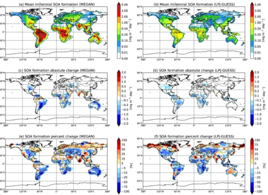
sions, averaged over the years 1000–2000. The area enclosed by the red contour represents regions with SOA formation rates greater than 5 % of the maximum mean millennial SOA formation from emissions of all BVOCs (isoprene, monoter-penes, and sesquiterpenes). Isoprene (Fig. 3a) has the largest contribution to SOA formation with a global millennial mean contribution of 64 %. Regions where isoprene emissions have significant contributions to SOA formation (greater than 70 %) are collocated with regions of highest total SOA for-mation (red contour). This shows that isoprene emissions are the predominant simulated source of global biogenic SOA formation, despite having the lowest SOA production yield of the three BVOCs. Some global models (e.g., D’Andrea et al., 2013; Lee et al., 2013) use monoterpene emissions as a representative BVOC for SOA formation rather than isoprene which may introduce errors in the spatial distribution and amount of biogenic SOA. Monoterpene emissions (Fig. 3b) contribute to 20 % of global mean millennial SOA forma-tion. Figure 3b indicates that monoterpene emissions are the most important source of SOA in the Northern Hemisphere boreal-forested regions, with contributions exceeding 80 %. However, monoterpenes contribute less than 20 % in regions with the highest total SOA formation. Sesquiterpene emis-sions represent the smallest global mean contribution to SOA formation at 16 % over the past millennium. Unlike isoprene
and monoterpene emissions that have clear regional impor-tance, Fig. 3c indicates that sesquiterpene emissions tend to have a more uniform contribution to SOA formation across all vegetated regions, but rarely exceeding 20 %.
4.2 Impact on aerosol number: changing BVOC emissions
Table 2.Summary of global, annual mean percent changes in N3, N10, N40, and N80 (number of particles with diameter greater than 3, 10, 40, and 80 nm, respectively) when changing BVOC emissions from year 1000 to year 2000 using the MEGAN and LPJ-GUESS reconstructions. The values in brackets are the global maximum and minimum percent changes.
MEGAN LPJ-GUESS
BE2.AEO– BE2.AE2– BE2.AEO.up– BE2.AE2.up– BE2.XSOA– BE2.AEO.LPJ–
BE1.AEO BE1.AE2 BE1.AEO.up BE1.AE2.up BE1.XSOA BE1.AEO.LPJ
N3 3.2 % 2.3 % 4.6 % 3.6 % 1.9 % 5.9 %
(40 %,−10 %) (49 %,−21 %) (53 %,−10 %) (59 %,−27 %) (26 %,−3 %) (63 %,−17 %)
N10 1.9 % 1.5 % 2.6 % 2.6 % 1.2 % 3.5 %
(38 %,−25 %) (29 %,−13 %) (40 %,−29 %) (34 %,−18 %) (17 %,−2 %) (36 %,−13 %)
N40 0.4 % −0.6 % 1.1 % −0.0 % 0.3 % −0.1 %
(28 %,−23 %) (18 %,−42 %) (45 %,−44 %) (20 %,−41 %) (8 %,−14 %) (24 %,−28 %)
N80 −0.6 % −1.3 % 0.0 % −1.2 % −0.3 % −1.8 %
(20 %,−28 %) (21 %,−43 %) (33 %,−24 %) (25 %,−40 %) (5 %,−21 %) (34 %,−36 %)
180° 120°W 60°W 0° 60°E 120°E 180°
180° 180°
90°S 60°S 30°S 0° 30°N 60°N
90°N (a) Contribution to SOA formation from isoprene
180° 120°W 60°W 0° 60°E 120°E 180°
180° 180°
90°S 60°S 30°S 0° 30°N 60°N
90°N (b) Contribution to SOA formation from monoterpenes
180° 120°W 60°W 0° 60°E 120°E 180°
180° 180°
90°S 60°S 30°S 0° 30°N 60°N
90°N (c) Contribution to SOA formation from sesquiterpenes
10 20 30 40 50 60 70 80 90 100
[%]
Figure 3. Percent contribution to SOA formation by (a) iso-prene,(b)monoterpene, and(c)sesquiterpene emissions from the MEGAN reconstruction, averaged over the years 1000–2000. The area enclosed by the red contour represents greater than 5 % of the maximum mean millennial SOA formation from emissions of BVOCs (isoprene, monoterpenes, and sesquiterpenes).
There are decreases in N80 exceeding 25 % in regions such as southern South America, southern Africa, southeastern North America, and Australia. These regions coincide with regions of significant decrease in isoprene emissions (Fig. 1) and SOA formation (Fig. 2). The relationship between the decrease in isoprene emissions and SOA formation with the decrease in N80 and increase in N3 and N10 can be explained through microphysical feedback mechanisms. Firstly, the de-crease in total isoprene emissions in these regions causes a decrease in SOA formation as explained in Sect. 4.1. With decreases in SOA formation, ultrafine particle growth de-creases due to the reduction in available condensable mate-rial. This can be seen in Fig. 4a and b where increases in N3 and N10 are collocated. This suppression of ultrafine parti-cle growth limits the number of partiparti-cles that can grow to CCN sizes, hence decreasing N80 in these regions. A reduc-tion in the number of N80 reduces the coagulareduc-tion sink of smaller particles, and N3 and N10 increase. This can be seen in Fig. 4, where regions of increasing N3 and N10 coincide with regions of decreasing N40 and N80. Throughout these regions, N3 and N10 increases exceed 25 %, and decreases in N40 and N80 exceed 25 %. These are significant changes in CCN concentrations (N40 and N80) in these regions due largely to changes in BVOCs due to anthropogenic land-use changes. With significant decreases in N40 and N80, the condensation sink for sulfuric acid (H2SO4)and coagulation
sink for ultrafine particles also decreases. This increases the survival probability of ultrafine particles and hence increases N3 and N10. Secondly, with a decrease in SOA formation and a decrease in ultrafine particle growth, the concentration of sulfuric acid (H2SO4)vapor increases in these regions due
to a decrease in the condensation sink. This increases nucle-ation due to the strong dependence on H2SO4vapor
180° 120°W 60°W 0° 60°E 120°E 180°
180° 180°
90°S 60°S 30°S 0° 30°N 60°N
90°N (a) N3 BL % change
50.0 25.0 10.0 5.0 1.0 0.5 0.5 1.0 5.0 10.0 25.0 50.0
[%]
180° 120°W 60°W 0° 60°E 120°E 180°
180° 180°
90°S 60°S 30°S 0° 30°N 60°N
90°N N10 BL % change
180° 120°W 60°W 0° 60°E 120°E 180°
180° 180°
90°S 60°S 30°S 0° 30°N 60°N
90°N (c) N40 BL % change
180° 120°W 60°W 0° 60°E 120°E 180°
180° 180°
90°S 60°S 30°S 0° 30°N 60°N
90°N N80 BL % change
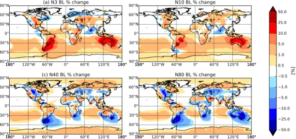
Figure 4.Percentage change in annually averaged boundary layer(a)N3,(b)N10,(c)N40, and(d)N80 (number of particles with diameter greater than 3, 10, 40, and 80 nm, respectively) when changing MEGAN BVOC emissions from year 1000 to year 2000 with constant present-day anthropogenic emissions (2005) (BE2.AE2.meg–BE1.AE2.meg). Globally averaged, N3 and N10 increased by 2.3 and 1.5 %, respectively, whereas N40 and N80 decreased by 0.6 and 1.3 %, respectively (see Table 2). An increase in particle number concentration is represented in red, and a decrease in blue.
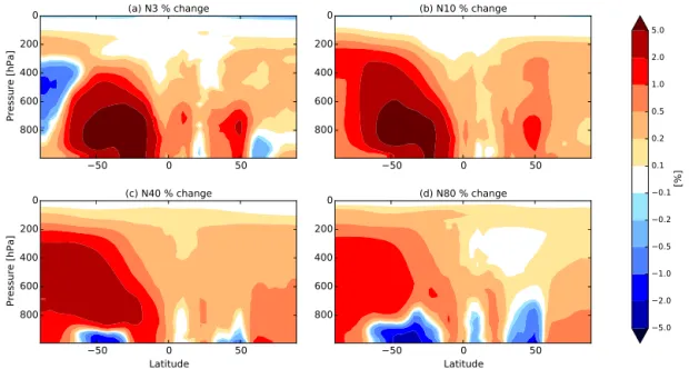
There are also increases in N80 over oceanic regions downwind of regions with significant decreases in N80. This is caused by the increases in N3 and N10 over land. When the air mass is advected over the ocean, the surplus of small particles are able to grow via condensation to CCN sizes. Figure 5 shows the zonal-mean percentage change in (a) N3, (b) N10, (c) N40, and (d) N80 when changing MEGAN BVOC emissions from year 1000 to year 2000 with constant present-day anthropogenic emissions (2005) (BE2.AE2.meg–BE1.AE2.meg). Figure 5 indicates that the difference in number concentrations between the two sim-ulations varies with height. The difference in N3 and N10 between the simulations with height generally remains pos-itive above the boundary layer (BL), with increases exceed-ing 5 % in the southern mid-latitudes in oceanic and defor-ested regions particularly. However, the differences in N40 and N80 between the simulations reverse sign with height in the mid-latitudes, most dramatically in the Southern Hemi-sphere such that there are more particles in the BE2.AE2.meg simulation. When CCN-sized particles are removed through wet deposition during vertical advection, there are more ul-trafine particles to grow to CCN sizes and replace the lost CCN in the BE2.AE2.meg simulation than in BE1.AE2.meg. This feedback leads to the change in sign with height for N40 and N80. This reversal in the change in particle number con-centrations has implications for radiative forcing and will be discussed in Sect. 4.3.
Figure 6 shows the change in (a) N3, (b) N10, (c) N40, and (d) N80 when changing MEGAN BVOC emissions from year 1000 to year 2000 with anthropogenic emissions turned off (BE2.AEO.meg–BE1.AEO.meg). Globally
aver-aged, N3, N10, and N40 increased by 3.2, 1.9, and 0.4 %, respectively, whereas N80 decreased by 0.6 % (see Table 2). Similar to the previous case, globally averaged N3 and N10 increased over the past millennium. However, contrary to the previous case, with anthropogenic emissions turned off, globally averaged N40 also increased. The spatial patterns in globally averaged number of CCN-sized particles (N80) in this simulation reflected the same decreasing trend as shown in Fig. 4. In Fig. 6, the regions of increasing N3 and N10 coincide with regions of decreasing N40 and N80, follow-ing the same spatial pattern as in Fig. 4. Thus, the presence of anthropogenic aerosols does not qualitatively change the fractional response of the aerosol size distribution to millen-nial changes in BVOCs.
There-50 0 50 0
200
400
600
800
Pressure [hPa]
(a) N3 % change
50 0 50
0
200
400
600
800
(b) N10 % change
50 0 50
Latitude 0
200
400
600
800
Pressure [hPa]
(c) N40 % change
50 0 50
Latitude 0
200
400
600
800
(d) N80 % change
5.0 2.0 1.0 0.5 0.2 0.1 0.1 0.2 0.5 1.0 2.0 5.0
[%]
Figure 5.Zonal-mean annual-average percentage change in(a)N3,(b)N10,(c)N40, and(d)N80 when changing MEGAN BVOC emissions
from year 1000 to year 2000 with constant present-day anthropogenic emissions (2005) (BE2.AE2.meg–BE1.AE2.meg). An increase in particle number concentration is represented in red, and a decrease in blue.
180° 120°W 60°W 0° 60°E 120°E 180°
180° 180°
90°S 60°S 30°S 0° 30°N 60°N
90°N (a) N3 BL % change
50.0 25.0 10.0 5.0 1.0 0.5 0.5 1.0 5.0 10.0 25.0 50.0
[%]
180° 120°W 60°W 0° 60°E 120°E 180°
180° 180°
90°S 60°S 30°S 0° 30°N 60°N
90°N N10 BL % change
180° 120°W 60°W 0° 60°E 120°E 180°
180° 180°
90°S 60°S 30°S 0° 30°N 60°N
90°N (c) N40 BL % change
180° 120°W 60°W 0° 60°E 120°E 180°
180° 180°
90°S 60°S 30°S 0° 30°N 60°N
90°N N80 BL % change
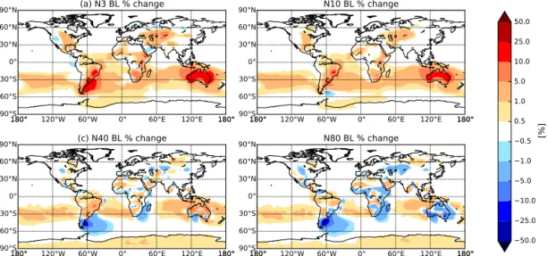
Figure 6.Percentage change in annually averaged boundary layer(a)N3,(b)N10,(c)N40, and(d)N80 when changing MEGAN BVOC emissions from year 1000 to year 2000 with anthropogenic emissions off (BE2.AEO.meg–BE1.AEO.meg). Globally averaged, N3, N10, and N40 increased by 3.2, 1.9, and 0.4 %, respectively, whereas N80 decreased by 0.6 % (see Table 2). An increase in particle number concentration is represented in red, and a decrease in blue.
fore, there are an increased number of ultrafine particles com-peting for condensation of SOA and growth to CCN sizes in the simulations with anthropogenic emissions on, and the particles in these simulations are (on average) smaller and further from CCN sizes than simulations with anthropogenic emissions off. Thus, ultrafine particles grow to CCN sizes more efficiently in the simulations with anthropogenic emis-sions turned off and are more susceptible to BVOC emission changes because there are fewer particles competing for
con-densable material and the mean size is larger. The fractional changes in N3 are larger in the cases with anthropogenic emissions off because there are fewer particles overall. Thus, there is a smaller increase in N3 and larger decrease in N80 than with anthropogenic emissions turned off.
10-8 10-7 10-6 Dp [m]
0 500 1000 1500 2000 2500
dN/d
log10 Dp
[c
m
−
3]
BE2.AE2.meg BE1.AE2.meg BE2.AEO.meg BE1.AEO.meg BE2.AE2.up BE1.AE2.up BE2.AEO.up BE1.AEO.up BE2.XSOA BE1.XSOA BE2.AEO.LPJ BE1.AEO.LPJ ¯
Dp,BE2.AE2.meg (30.6 nm)
¯
Dp,BE2.AEO.meg (52.1 nm)
¯
Dp,BE2.AE2.up (35.6 nm)
¯
Dp,BE2.AEO.up (68.5 nm)
¯
Dp,BE2.XSOA (85.9 nm)
¯
Dp,BE2.AEO.LPJ (63.6 nm)
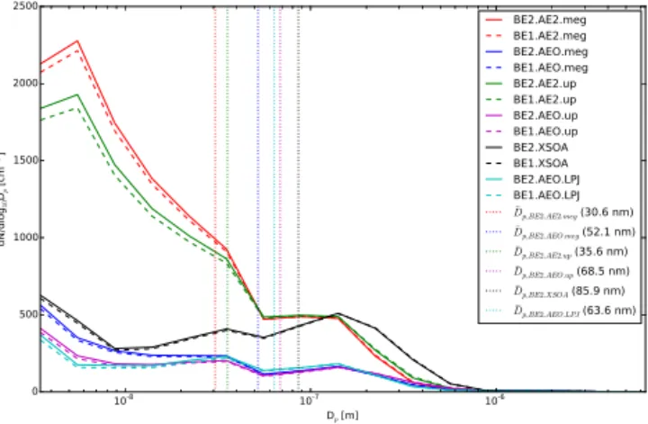
Figure 7. Simulated global boundary layer annual-mean par-ticle number size distributions for the simulations outlined in Table 1. The vertical dotted lines represent the mean di-ameter for the simulations using year 2000 biogenic emis-sions (BE2.AE2.meg, BE2.AEO.meg, BE2.AE2.up, BE2.AEO.up, BE2.XSOA, and BE2.AEO.LPJ).
from pre-industrial (off) to present-day (2005) with con-stant present-day BVOC emissions (average biogenic emis-sions from 1980–1990) (BE2.AE2.meg–BE2.AEO.meg) in-creased by 382, 339, 212, and 162 %, respectively. These global sensitivities to anthropogenic emissions changed only modestly when biogenic emissions from 1000 were used (BE1.AE2.meg–BE1.AEO.meg): globally averaged N3, N10, N40, and N80 all increased by 386, 341, 215, and 164 %, respectively. The global millennial change in particles due to BVOC changes is small compared to the change in an-thropogenic emissions; however, the change in particles due to changes in BVOC is still non-trivial, and we will discuss this further when discussing radiative forcing. This empha-sizes the importance of accurately quantifying the aerosols in the pre-industrial reference state used for radiative forcing calculations (Carslaw et al., 2013)
The sensitivity of particle numbers to upper bounds on SOA yields was also investigated. The fixed SOA yields used in the standard simulations (3, 10, and 20 % for isoprene, monoterpenes, and sesquiterpenes, respectively) were increased to 10, 20, and 40 % for isoprene, monoter-penes, and sesquitermonoter-penes, respectively, in the upper-bound simulations (BE2.AEO.up, BE1.AEO.up, BE2.AE2.up, and BE1.AE2.up). When using the upper-bound SOA yields and changing MEGAN BVOC emissions from year 1000 to year 2000 with anthropogenic emissions turned off (BE2.AEO.up–BE1.AEO.up), globally averaged N3, N10, N40, and N80 increased by 4.6, 2.6, 1.1, and 0.0 %, respec-tively (see Table 2). The spatial distribution of the global changes in particle number concentrations are similar to those of Fig. 4, with modest increases in magnitude. Even with more than a doubling of the SOA yields from all three terpenoid species, the change in particle number responded
with less than a doubling due to microphysical dampening. This has also been observed in other global aerosol micro-physics models (e.g., Scott et al., 2014). With an increase in SOA yields, there is a corresponding increase in the amount of condensable material available for particle growth. How-ever, due to the nonlinear balance between condensational growth and coagulational scavenging, increases in particle number concentrations do not scale linearly with increases in SOA formation.
This microphysical feedback was also seen when using upper-bound SOA yields while changing MEGAN BVOC emissions from year 1000 to year 2000 with present-day an-thropogenic emissions (2005) (BE2.AE2.up–BE1.AE2.up). Globally averaged, N3 and N10 increased by 3.6 and 2.6 %, respectively, whereas N40 and N80 decreased by 0.0 and 1.2 %, respectively (see Table 2). This comparison showed the same spatial patterns as the standard yield comparison of Fig. 6 with modest increases in magnitude similar to the simulations with anthropogenic emissions off. The nonlin-ear impact on global particle number concentrations due to microphysical dampening was also observed in this compari-son. Therefore, due to the similarity of the upper-bound SOA yield simulations to the standard SOA yield simulations, we have not included these in the figures. However, the SOA yields will also likely not remain constant since they will change with varying conditions such as aerosol loading or NOxconcentrations.
SOA cases (BE2.XSOA–BE1.XSOA) to the standard cases (BE2.AE2.meg–BE1.AE2.meg) are lower in magnitude (see Table 2).
Figure 9 shows the change in (a) N3, (b) N10, (c) N40, and (d) N80 when changing LPJ-GUESS BVOC emissions from year 1000 to year 2000 with anthropogenic emissions off (BE2.AEO.LPJ–BE1.AEO.LPJ), providing an estimate for the aerosol changes when using an independent estimate of BVOC changes. Globally averaged, N3 and N10 increased by 5.9 and 3.5 %, respectively, whereas N40 and N80 de-creased by 0.1 and 1.8 %, respectively (see Table 2). The magnitude of the changes in N3 and N80 with the LPJ-GUESS simulations are the highest of all the simulations. This is due in part to the spatial variability in the LPJ-GUESS emission inventory when compared to the MEGAN emis-sion inventory, as well as lower total emisemis-sions. Similar to the comparable simulations using the MEGAN emissions (BE2.AEO.meg–BE1.AEO.meg; Fig. 6), there are increases in N3 over central North America, southern South America, eastern Australia, and central Eurasia exceeding 25 %. These regions correspond to regions of decreased BVOC emissions over the past millennium, which leads to decreases in SOA formation and increases in N3 (due to the deficit of con-densable material available to grow the smallest particles to CCN sizes). The same regions with significant increases in N3 also correspond to regions of significant decreases in CCN-sized particles. However, there are regions where the MEGAN simulations and the LPJ-GUESS simulations dif-fer. Even though LPJ-GUESS emits less BVOC emissions globally than MEGAN, the LPJ-GUESS simulations indi-cate higher-magnitude increases in N3 in the Northern Hemi-sphere than MEGAN. This is due to LPJ-GUESS emitting relatively more BVOCs in the northern boreal-forested re-gions than MEGAN (largely due to the different emission factors assumed for vegetation types and the treatment of the CO2 response of the two emission models), and
there-fore increased SOA formation. This is reflected in the global mean size distribution (Fig. 7) where it can be seen that BE2.AEO.LPJ has fewer small particles than BE2.AEO.meg, confirmed by a larger mean diameter at 63.6 nm as opposed to 52.1 nm for BE2.AEO.meg. Overall, the percent change in N80 between the LPJ-GUESS and MEGAN simulations have a correlation coefficient of 0.49. The previously men-tioned regional differences between the two BVOC recon-structions are a source of uncertainty, but the global percent change in N80 both follow the same trend (Table 2). This indicates that anthropogenic land-use changes over the past millennium have decreased the number of CCN-sized parti-cles globally through changes in BVOC emissions, with re-gional changes in CCN-sized particles ranging from−25 to 25 %.
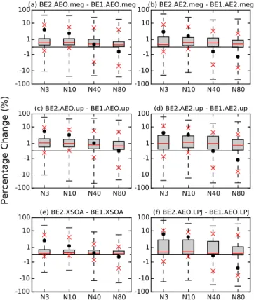
The distribution of changes across all grid boxes in N3, N10, N40, and N80 for all simulations are summarized in Fig. 10 (see Table 2 for specific values). Plotted are the global percent changes in N3, N10, N40, and N80 for
bio-genic emissions from 1000 to 2000 on a logarithmic scale. For all of the simulation comparisons, there is an increase in mean N3 and a decrease in mean N80. This is due mainly to the decrease in isoprene emissions over the past millennium, predominantly influenced by land-use changes. However, the majority of the changes globally are very close to zero (as can be seen by the size of the interquartile range on all plots). This is caused by minute changes in number concentrations over open ocean regions. Also, there is significant variability in the magnitude of the changes in all simulations as can be seen by the extent of the maximum and minimum changes in particle number concentrations. This indicates that cau-tion must be taken when interpreting global mean values, as regional changes are of importance.
4.3 Aerosol direct and indirect radiative effects
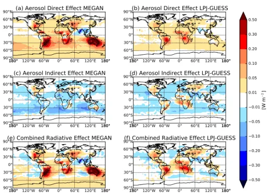
Figure 11 shows the annual mean radiative effect due to changes in BVOC emissions between year 1000 and year 2000 (see Table 3 for summarization). Figure 11a shows the DRE due to changing BVOC emissions between year 1000 and year 2000 with MEGAN BVOC emissions and anthro-pogenic emissions off (BE2.AEO.meg–BE1.AEO.meg), giv-ing a global annual mean DRE of +0.065 W m−2. While this global-mean DRE from biogenic emissions changes is smaller in magnitude than estimated anthropogenic direct ra-diative forcings (e.g., estimates of−0.85 to+0.15 W m−2 in the most recent IPCC report, Boucher et al. 2013), the DRE from biogenic emissions changes may be much larger regionally. Throughout most oceanic regions, the DRE is small (< 0.05 W m−2); however, over land there are large re-gions experiencing a DRE greater than +0.5 W m−2 (e.g., southeastern South America, southern Africa, Australia, and southeastern North America). This is caused by significant decreases in N80 (as seen in Fig. 6) and the total mass of particles (not shown), which decreases the scattering of in-coming solar radiation. There are regions of negative radia-tive forcing (e.g., India), which are associated with increases in N80 and total aerosol mass due to increased BVOC emis-sions from the anthropogenic introduction of high BVOC-emitting plants and cropland. There is a band of positive ra-diative forcing in the Southern Hemisphere, which is associ-ated with mid-latitude westerlies transporting accumulation-mode particles over oceanic regions.
magni-180° 120°W 60°W 0° 60°E 120°E 180°
180° 180°
90°S 60°S 30°S 0° 30°N 60°N
90°N (a) N3 BL % change
50.0 25.0 10.0 5.0 1.0 0.5 0.5 1.0 5.0 10.0 25.0 50.0
[%]
180° 120°W 60°W 0° 60°E 120°E 180°
180° 180°
90°S 60°S 30°S 0° 30°N 60°N
90°N N10 BL % change
180° 120°W 60°W 0° 60°E 120°E 180°
180° 180°
90°S 60°S 30°S 0° 30°N 60°N
90°N (c) N40 BL % change
180° 120°W 60°W 0° 60°E 120°E 180°
180° 180°
90°S 60°S 30°S 0° 30°N 60°N
90°N N80 BL % change
Figure 8.Percentage change in annually averaged boundary layer(a)N3,(b)N10,(c)N40, and(d)N80 when changing MEGAN BVOC
emissions from year 1000 to year 2000 with constant present-day anthropogenic emissions (2005) including an additional 100 Tg SOA yr−1
as per D’Andrea et al. (2013) (BE2.XSOA–BE1.XSOA). Globally averaged, N3, N10, and N40 increased by 1.9, 1.2, and 0.3 %, respectively, whereas N80 decreased by 0.3 % (see Table 2). An increase in particle number concentration is represented in red, and a decrease in blue.
180° 120°W 60°W 0° 60°E 120°E 180°
180° 180°
90°S 60°S 30°S 0° 30°N 60°N
90°N (a) N3 BL % change
50.0 25.0 10.0 5.0 1.0 0.5 0.5 1.0 5.0 10.0 25.0 50.0
[%]
180° 120°W 60°W 0° 60°E 120°E 180°
180° 180°
90°S 60°S 30°S 0° 30°N 60°N
90°N N10 BL % change
180° 120°W 60°W 0° 60°E 120°E 180°
180° 180°
90°S 60°S 30°S 0° 30°N 60°N
90°N (c) N40 BL % change
180° 120°W 60°W 0° 60°E 120°E 180°
180° 180°
90°S 60°S 30°S 0° 30°N 60°N
90°N N80 BL % change
Figure 9.Percentage change in annually averaged boundary layer(a)N3,(b)N10,(c)N40, and(d)N80 when changing LPJ-GUESS BVOC emissions from year 1000 to year 2000 with anthropogenic emissions off (BE2.AEO.LPJ–BE1.AEO.LPJ). Globally averaged, N3 and N10 increased by 5.9 and 3.5 %, respectively, whereas N40 and N80 decreased by 0.1 and 1.8 %, respectively (see Table 2). An increase in particle number concentration is represented in red, and a decrease in blue.
tude (due to smaller emissions changes). However, there is a large difference in DRE between MEGAN and LPJ-GUESS over Australia. This is due to a decrease in emissions from MEGAN between year 1000 and year 2000, resulting in a decrease in SOA formation and leading to a strong posi-tive DRE. However, there are smaller magnitude changes in emissions from LPJ-GUESS, which are due to a combination of inland increases and coastal decreases (mainly caused by changes in isoprene emissions), leading to a combination of increases and decreases in N80 over Australia.
radia-Table 3.Summary of global, annual mean changes in aerosol direct radiative effect (DRE), first aerosol indirect effect (AIE), and combined radiative effect in W m−2when changing BVOC emissions from year 1000 to year 2000 using the MEGAN and LPJ-GUESS reconstructions.
The values in brackets are the global maximum and minimum changes, respectively.
MEGAN LPJ-GUESS
BE2.AEO– BE2.AE2– BE2.AEO.up– BE2.AE2.up– BE2.XSOA– BE2.AEO.LPJ–
BE1.AEO BE1.AE2 BE1.AEO.up BE1.AE2.up BE1.XSOA BE1.AEO.LPJ
DRE +0.065 +0.050 +0.129 +0.163 +0.052 +0.022
[W m−2] (−0.305,+1.008) (−0.394,+1.005) (−0.521,+1.806) (−0.934,+2.020) (−0.377,+0.985) (−0.059,+0.381)
AIE∗ −0.020 −0.035 −0.035 −0.056 −0.025 −0.008
[W m−2] (−0.175,+0.201) (−0.262,+0.406) (−0.291,+0.212) (−0.369,+0.154) (−0.288,+0.108) (−0.156,+0.285)
Combined radiative +0.049 +0.022 +0.101 +0.118 +0.032 +0.015
effect∗[W m−2] (−0.316,+1.019) (−0.394,+1.005) (−0.547,+1.808) (−0.930,+1.970) (−0.382,+0.973) (−0.122,+0.436)
∗Cloud drop number concentrations were calculated using a globally uniform updraft velocity of 0.2 m s−1.
N3 N10 N40 N80
-100-10
-1 1 10
100(a) BE2.AEO.meg - BE1.AEO.meg
N3 N10 N40 N80
-100-10
-1 1 10
100(b) BE2.AE2.meg - BE1.AE2.meg
N3 N10 N40 N80
-100-10
-1 1 10
100 (c) BE2.AEO.up - BE1.AEO.up
N3 N10 N40 N80
-100-10
-1 1 10
100 (d) BE2.AE2.up - BE1.AE2.up
N3 N10 N40 N80
-100-10
-1 1 10
100 (e) BE2.XSOA - BE1.XSOA
N3 N10 N40 N80
-100-10
-1 1 10
100 (f) BE2.AEO.LPJ - BE1.AEO.LPJ
Percentage Change (%)
Figure 10. Global percent changes in N3, N10, N40, and N80 for biogenic emissions from 1000 to 2000 on a logarithmic scale for the simulations (a) BE2.AEO.meg–BE1.AEO.meg,(b)
BE2.AE2.meg–BE1.AE2.meg, (c), BE2.AEO.up–BE1.AEO.up,
(d) BE2.AE2.up–BE1.AE2.up, (e) BE2.XSOA–BE1.XSOA, and
(f) BE2.AEO.LPJ–BE1.AEO.LPJ. The black dots indicate the
global mean, the red line is the global median, the grey boxes are the interquartile range, the whiskers are the global maximum and min-imum changes and the red Xs indicate the 5th and 95th percentiles (see Table 2).
tive forcing associated with increases in N80 in both the Southern Hemisphere and Northern Hemisphere mid-latitude westerlies with regional cloud-albedo AIEs in excess of
−0.10 W m−2. The subtropical marine clouds in these re-gions are sensitive to changes in CCN number concentration, giving a strong cooling effect. This band of negative radia-tive forcing is caused by increased number concentrations of CCN-sized particles (N40 and N80) above the BL (Fig. 5). The increases in CCN-sized particles aloft causes increases in CDNC in the vertical layers with the highest cloud frac-tions (∼700 hPa) and thus a net cooling effect. There are also regions that experience a small positive cloud-albedo AIE due to changing BVOC emissions (e.g., southeastern North America, western Europe, and southeastern Australia) asso-ciated with regions of decreased N80.
0.50 0.30 0.20 0.10 0.05 0.01 0.01 0.05 0.10 0.20 0.30 0.50
[W
m
−
2]
180° 120°W 60°W 0° 60°E 120°E 180°
180° 180°
90°S 60°S 30°S0° 30°N 60°N
90°N
(a) Aerosol Direct Effect MEGAN
180° 120°W 60°W 0° 60°E 120°E 180°
180° 180°
90°S 60°S 30°S0° 30°N 60°N
90°N
(b) Aerosol Direct Effect LPJ-GUESS
180° 120°W 60°W 0° 60°E 120°E 180°
180° 180°
90°S 60°S 30°S0° 30°N 60°N
90°N
(c) Aerosol Indirect Effect MEGAN
180° 120°W 60°W 0° 60°E 120°E 180°
180° 180°
90°S 60°S 30°S0° 30°N 60°N
90°N
(d) Aerosol Indirect Effect LPJ-GUESS
180° 120°W 60°W 0° 60°E 120°E 180°
180° 180°
90°S 60°S 30°S0° 30°N 60°N
90°N
(e) Combined Radiative Effect MEGAN
180° 120°W 60°W 0° 60°E 120°E 180°
180° 180°
90°S 60°S 30°S0° 30°N 60°N
90°N
(f) Combined Radiative Effect LPJ-GUESS
Figure 11.Annual mean change between year 1000 and year 2000 in(a)DRE with MEGAN BVOC emissions and anthropogenic emis-sions off (BE2.AEO.meg–BE1.AEO.meg),(b)DRE with LPJ-GUESS BVOC emissions and anthropogenic emissions off (BE2.AEO.LPJ–
BE1.AEO.LPJ),(c)AIE with MEGAN BVOC emissions and anthropogenic emissions off,(d)AIE with LPJ-GUESS BVOC emissions and anthropogenic emissions off,(e)combined radiative effect with MEGAN BVOC emissions and anthropogenic emissions off, and(f)
combined radiative effect with LPJ-GUESS BVOC emissions and anthropogenic emissions off. Global mean changes are+0.065,+0.022, −0.020,−0.008,+0.049, and+0.015 W m−2, respectively (see Table 3).
warming of +0.015 W m−2. Similar to Fig. 11e, the AIE cooling effect over oceanic regions is balanced by the warm-ing effect in the same regions due to the increases in DRE. Therefore, the warming effect from the DRE dominates the total radiative effect. The additional significance of Fig. 11 is that it shows the forcing error resulting from holding bi-ological emissions fixed when calculating anthropogenic ra-diative forcings from pre-industrial to the present day. Thus, the error in the anthropogenic forcing maybe on the order of 0.5 W m−2over various regions if these changes in biogenic emissions are not included.
We also explored the aerosol radiative effect under the assumption of bound SOA yields. With this upper-bound yield changing MEGAN BVOC emissions from year 1000 to year 2000 with present-day anthropogenic emis-sions (2005) (BE2.AE2.up–BE1.AE2.up) resulted in a global mean DRE of +0.163 W m−2 (a factor 3.2 greater than un-der standard SOA yields) and the global mean cloud-albedo AIE to−0.056 W m−2(factor 1.6 greater than standard SOA yield). The radiative effect due to changing BVOC emissions is therefore sensitive to assumptions about SOA yield.
4.4 Discussion of model limitations
There are certain limitations associated with our assump-tions and model setup used in this study. Organic emissions
do not participate in the nucleation process within GEOS-Chem-TOMAS; however, the inclusion of oxidized organic vapors may increase the sensitivity of particle number con-centrations to changes in BVOC emissions, particularly in monoterpene-emitting regions known to produce extremely low volatile organic compounds (Riccobono et al., 2014; Scott et al., 2014). This inclusion of organic vapors in the nu-cleation process would also increase the pre-industrial (year 1000) baseline number concentrations (Scott et al., 2014). The SOA yields in GEOS-Chem-TOMAS are fixed; how-ever, these yields may change with total organic mass, NOx
concentrations, and changes in atmospheric oxidants. The change in SOA formation has no influence on the oxidation fields in GEOS-Chem-TOMAS and, therefore, there may be missing feedback mechanisms on key atmospheric oxi-dants as BVOCs are removed from the model system without changing model OH concentrations. This model also ignores OH recycling mechanisms that may accompany changes in isoprene oxidation, which may impact oxidation rates and SOA yields. SOA formation by NO3is not included in this
model – while this is likely minor for much of the globe, we may be underestimating SOA formed in areas influenced by monoterpenes and NOx. Also, the inclusion of an additional
an-thropogenically enhanced SOA will cause additional uncer-tainties in our predictions, by changing the organic aerosol mass, which affect SOA growth rates and yields. The BVOC reconstructions also inherently have uncertainties associated with them. The response of plant emissions to environmen-tal changes including CO2 and temperature is contentious,
particularly with respect to monoterpene and sesquiterpene emission. Plant BVOC emissions respond differently to CO2
exposure in the short-term vs. CO2 exposure in the
long-term (i.e., BVOC emissions of plants exposed to elevated CO2 for minutes or hours are different from BVOC
emis-sions plants exposed to elevated CO2from seed germination)
(Heald et al., 2009). Perhaps more important for this study, the temperature dependence of BVOC emissions included in the emission models are typically based on short-term leaf-level exposure, and ignore the potential for plants to adapt to increasing temperature. Both MEGAN and LPJ-GUESS have been separately evaluated against observations (Arneth et al., 2007; Schurgers et al., 2009; Guenther et al., 2006) and compared to each other (Arneth et al., 2011; Guenther et al., 2012); however, without long-term measurements of BVOC fluxes there may be bias in the reconstructions towards the available short-term measurements used to develop the re-constructions. Experimental limitations in emission factors for the various plant functional types used to create the re-construction also lead to uncertainties in the BVOC recon-structions. Finally, there is no way to directly test the emis-sions for the historic simulations. We expect the general spa-tial patterns to be robust, not necessarily the magnitudes.
5 Conclusions
In this study, we investigated the impact of millennial changes in biogenic volatile organic compound (BVOC) emissions on secondary organic aerosol (SOA) formation and global aerosol size distributions, and we calculated the associated aerosol radiative forcing. We used the global aerosol microphysics model GEOS-Chem-TOMAS to con-nect the historical changes in BVOC emissions to particle size distributions and the number concentration of cloud con-densation nuclei (CCN).
This study built off recent work by Acosta Navarro et al. (2014), who determined how BVOC emissions have changed in the past millennium due to changes in land use, temperature, and carbon dioxide (CO2)concentrations.
They used two model reconstructions including three dom-inant classes of BVOC emissions (isoprene, monoterpenes, and sesquiterpenes) to simulate decadal-averaged monthly mean emissions over the time period 1000–2000. Their emissions reconstructions predicted that isoprene emissions decreased over the past millennium (due mainly to an-thropogenic land-use changes), whereas monoterpene and sesquiterpene emissions increased (due predominantly to temperature increases). In our work, we included these
mil-lennial emissions into the GEOS-Chem-TOMAS chemical-transport model with online aerosol microphysics for SOA production only (no influence on the oxidant fields). We as-sumed that isoprene, monoterpenes, and sesquiterpenes form SOA in GEOS-Chem-TOMAS via fixed yields of 3, 10, and 20 %, respectively.
When anthropogenic emissions (e.g., SO2, NOx,
pri-mary aerosols) were turned off to represent pre-industrial conditions and emissions of isoprene, monoterpenes, and sesquiterpenes changed from year 1000 values (“pre-industrial”) to year 2000 values (“present day”) using both BVOC reconstructions, N80 (the number of particles with diameter greater than 80 nm, our proxy for CCN in this study) had decreases of greater than 25 % in year 2000 rel-ative to year 1000 that were predicted in regions with ex-tensive land-use changes such as southern South America, southern Africa, southeastern North America, and southeast-ern Australia since year 1000. This significant change in N80 was predominantly driven by anthropogenic changes in high BVOC-emitting vegetation to lower-emitting crops/grazing land. Similar sensitivities in N80 exist when BVOC emis-sions were changed over the same time period but with an-thropogenic emissions set to present-day values. Including recent work by Spracklen et al. (2011) and D’Andrea et al. (2013), the sensitivity to an additional 100 Tg yr−1 of anthropogenically enhanced SOA was tested, with BVOC emissions changed from year 1000 to year 2000 values, re-sulting in globally averaged decreases in N80 of 0.3 %. How-ever, similar to the previous simulations, there are regional decreases exceeding 25 %. The sensitivity to SOA yields was also investigated by comparing simulations for year 1000 and 2000 BVOC emissions (with anthropogenic emissions both on and off) by increasing the yields from the base case of 3, 10, and 20 % for isoprene, monoterpenes, and sesquiterpenes to 10, 20, and 40 %, respectively. This significant increase (at least a doubling) in SOA formation resulted in a nonlinear increase in the magnitude of the changes in particle number concentrations of all sizes (doubling yields did not double changes in particle number concentrations); however, it con-firmed the same trend by globally decreasing N80. There are uncertainties in assuming fixed SOA yields however, as SOA yields are dependent on conditions such as aerosol loading and NOxconcentrations, and therefore it might not be fixed
with time.