ASSESSMENT OF THE HOMOGENEITY OF VOLUNTEERED GEOGRAPHIC
INFORMATION IN SOUTH AFRICA
L. Siebritza, G. Sitholeb, S. Zlatanovac
a
Chief Directorate: National Geospatial Information, van der Sterr Building, Rhodes Avenue, Mowbray, 7705, South Africa - lasiebritz@ruraldevelopment.gov.za
b
Geomatics Division, School of Architecture, Planning and Geomatics, University of Cape Town, Private Bag X3, Rondebosch, 7701, South Africa - george.sithole@uct.ac.za
c
GISt, OTB, Delft University of Technology, Jaffalaan 9, 2628 BX Delft, The Netherlands - s.zlatanova@tudelft.nl
KEYWORDS: Mapping, Updating, GIS, Comparison, Open Systems
ABSTRACT:
The potential for volunteer groups to contribute geographic data to National Mapping Agencies has been widely recognised. Several investigations have been done to determine the geometric accuracy of this data for the purposes of national mapping. Beyond accuracy, from a production perspective National Mapping Agencies will also be interested in the sufficiency and uniformity of the data. This paper presents an investigation of whether presently geographic data generated by volunteers is uniform across a country and whether the rate of production of data is consistent. For the purpose of the test, changes in data of South Africa from OpenStreetMap are analysed for the period 2006 to 2011. Here only point and line data are considered. The results generally show that the rate at which data is generated varies in space and time. The results also confirm that volunteers emphasise on the capture of certain information and that the capture doesn’t average out as might be expected. The results also showed that social events, such as a World Cup, also have the effect of spurring the generation of volunteer geographic data. The implication of these results for National Mapping Agencies is that they cannot treat volunteer geographic information as being of a uniform standard. How National Mapping Agencies respond to this will have to be the subject of other investigations.
1. INTRODUCTION
1.1 Background
The growth of social networking on the internet has led to the creation of collaborative geographic information systems. This democratization of spatial information has appealed to a community that is driven by an open knowledge philosophy and committed to the free sharing of knowledge. The distinct advantage of these communities is that because of their size they are able to generate vast quantities of current vector data. Goodchild (2007) and Goodchild & Glennon (2010) highlight that that each individual might act as a sensor and the crowd as a whole can be seen as a sensor network. Citizens can greatly support the process of data collection but the question arises: how trustful is the information they provide. Flanagin & Metzger (2008) suggest that volunteer efforts can be trusted relying on the ability of the crowd to detect and edit incorrect information. Heipke (2010) notes that mechanisms like in Wikipedia can be employed that will encourage this process. At the same time the author warns that information provided by locals tend to be of better quality compared to that gathered by volunteers unfamiliar with the environment.
National Mapping Agencies are the official custodians of geographic information and they have typically operated as closed systems. Because of the high costs of vector data extraction, the increasing demand for evermore current vector data and the emergence of collaborative GISs, National Mapping Agencies have been motivated to consider volunteer geographic data as a source of spatial information for map updating. Various studies have been done to determine the quantitative and qualitative qualities of spatial data generated by
a community of volunteers. Studies done so far, have examined volunteer geographic information against national
mapping standards. However, mapping is also influenced by personal and cultural traits. For example volunteers maybe motivated to capture only those features that are socially important to them such as schools and churches, and ignore other equally important land marks like museums and
restaurants. Unlike other studies that have sought to determine the geometric accuracies of volunteer geographic data, this paper sets out to answer a more fundamental question, “How differently do volunteers capture data ?”
1.2 Previous Work
Most VGI testing that has been done involves comparing VGI with official or survey data. This provides a good indication of the geometric accuracy of VGI within the test data. One of the VGI initiatives which have been tested by numerous researches is OpenStreetMap (OSM). The OSM repository has seen a rapid increase in volunteer contributions over the years. The data is also freely and easily available for testing. The types of contributions constitute mainly GPS data as collected by the public and vector data digitised off aerial and satellite imagery (Geofabrik 2011).
Haklay & Ellul (2010) did a comparative study between OSM and Ordnance Survey (OS) (the National Mapping Agency of Great Britain) in England for the period 2008-2009. The study measured completeness in terms of the total OSM line length compared to the OS data. The authors found that affluent areas see more contributions than socially excluded areas and there is an even bigger gap between areas of varying affluence when the comparison uses only attributed road features.
A study by AL Bakri, Fairbairn (2011) compared a subset of OSM data to OS data and field survey data was used as the reference data set to find (i) the geometric accuracy of the OSM data set and (ii) the semantic similarity between the OSM and OS data sets. The findings of the study were that the OSM data set had (i) a poor geometric accuracy and (ii) dissimilar semantics for the area of study.
The method by Haklay & Ellul (2010) was extended to France by Girres & Touya (2010), comparing OSM data to BD TOPO® data from Institut national de l’information géographique et forestière (IGN), but included several other assessments (e.g. temporal accuracy, logical consistency, lineage etc). Results showed that although the OSM data is a International Archives of the Photogrammetry, Remote Sensing and Spatial Information Sciences, Volume XXXIX-B4, 2012
good source of current geospatial data, there are limitations to the application of the data because of the lack of homogeneity.
Anand et al. (2010) compared OSM data the OS Integrated Transport Network (ITN) data for Portsmouth in the United Kingdom but with the focus on data integration. A prototype technique was developed that matches homologous feature pairs in the two datasets. The accuracy of the matching technique was found to have an 86% level of accuracy but, further testing is necessary to refine the results.
Zielstra and Zipf (2010) performed a comparative study between the OpenStreetMap and TeleAtlas MultiNet dataset for a number of cities in Germany. The investigations were completed on three data sets for 2009.The results revealed the length of the OSM streets is still smaller than the Tele Atlas street network. However, the OSM repository is growing at a remarkable rate, with a 22% increase in road length within only eight months.
The purpose of all the afore-mentioned studies is to estimate the reliability and quality of OSM data sets by comparing it to existing authoritive databases.
1.3 Objectives
The working principle of the paper is that for whatever reasons, volunteers will place different emphasis on spatial features and that this emphasis is carried through into the geographic data that they collect. This principle is tested using OpenStreetMap data. The paper studies only the homogeneity of volunteer geographic information and not the geometric uncertainties within volunteer geographic information. If it can be shown that this is the case then this will have profound implications for National Mapping Agencies. They can no longer assume that volunteer data is homogenous in feature types, space or time. As a consequence, the integration of national mapping data and volunteer data will have to be region, space and time specific or for the purpose of efficiency and quality control, the acquisition of data by volunteers will have to be standardized.
The paper is divided into six main sections. Section two looks at the method used to detect changes in the OSM data. Section three mentions the data sources. In section four the results are presented. Finally, sections five and six present the discussion and conclusions respectively.
2. COMPARISON METHOD
The OpenStreetMap (OSM) data sets are comprised of three geometry types: point, line and polygon. We have investigated the three geometry types separately. This paper presents our investigations on point and line data types only. We have defined four types of change: (i) Addition, i.e., where new data has been added (ii) Deletion, i.e., where existing data has been deleted, (iii) Modification, i.e., where the geometry of existing data has been modified and (iv) No Change, where there has been no geometric change between consecutive dates. In this study we have not considered changes of the thematic properties of a geometric feature. The determination of the changes for each geometry type is discussed below.
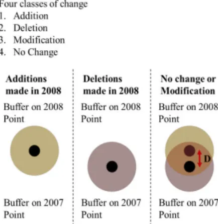
2.1 Categorising Point Data
The method of detecting changes in points is illustrated in Figure 1. To be able to determine the change, buffers are defined on the point features from the two dates being compared (for this example 2007 and 2008). Isolated 2008 points are
treated as additions. Isolated 2007 points are treated as deletions. Points contained in buffers are treated as modifications or no change. Modified points are those where the minimum distance D exceeds a defined threshold. Most VGI is captured by low cost GPS devices which are subject to an absolute positional accuracy of 5 m. Because of this a generous buffer of 3m was defined for the points. The implication of this is that any two points within 3 m of each other are treated as being the same feature. To determine modified points, the threshold on the distance D was set at 1 m. This threshold was chosen after calculating the standard deviation of the distance D for points that had not changed between the dates being compared. This was confirmed by visual inspection.
Figure 1 Determination of change in point geometry (e.g., location) between two dates.
2.2 Categorizing Line Data
The method of detecting changes in lines is illustrated in Figure 2. An approach similar to point geometry was followed. Square capped buffers were defined on the line features from the two dates being compared (for this example 2007 and 2008). The parts of the 2008 line not contained in the 2007 buffer are treated as additions. Similarly the parts of the 2007 line not contained in the 2008 buffer are treated as deletions. The remaining parts of the 2008 line are treated as modifications or no change. The modified parts of the 2008 line are where the minimum distance D exceeds a defined threshold. As with the points a buffer of 3m was defined for the lines. The implication of this is that any two lines within the buffer are being considered the same feature. To determine modified line segments the threshold on the distance D was set at 1 m. The threshold was defined on the basis of the standard deviation.
The summed lengths of the line segments for the different categories are calculated to quantify the changes between dates for each category. For the modified segments of the line the standard deviation of the interline distance D was calculated to obtain a measure of the amount of modification.
Figure 2 The determination of change in line geometry (e.g., roads) between two dates.
3. TEST DATA
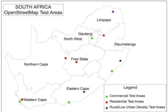
More than ten OSM data sets from cities and towns within South Africa (see Figure 3) were acquired for a period spanning from 2006 to 2011. Two data sets per year were used (for April and October) for year 2007 to 2011 and one data set from 2006, which gives 10 epochs. Eleven test areas have been determined as follows in: four large cities (Cape Town, Johannesburg, Durban, and Kimberley), three towns (Korsten, Middleburg and Stuttereheim), three suburbs (Brackenfell, Universitas and Gondeni) and one village (Makhwezini)),
From examinations of the thematic attributes of the data sets a category of spatial features has been defined (e.g., streets, residential, recreational, religious, business, educational, etc,). The test areas have been categorised into three groups namely
commercial (Cape Town, Johannesburg, Durban and Korsten),
residential (Brackenfell, Kimberley, Middelburg and
Universitas)) and low urban density areas (Gondeni, Makhwezini and Stutterehim). Aerial imagery was used to determine visually that each site was representative of the chosen categories. Each test area covered a square area of approximately 6.5 km2.
A timeline has been built for each test. The timelines show the category and quantity of features that have been collected for a given period of time (epoch). For example, epoch 1 is the period between June 2006 and Jan 2007, epoch 2 is from Jan 2007 to June 2007, etc. The timelines from the different data sets are then compared to determine (i) the features that are recorded at different stages of the development of a volunteer geographic data set (ii) the rate of development of a volunteer geographic data set (iii) and the variation in data collection for different regions, e.g. rural versus urban, industrial versus residential, etc.,.
Figure 3 Location of areas in South Africa from which the test areas are drawn.
4. RESULTS AND ANALYSIS
The tests were performed in ESRI ArcGIS environment using the standard operations: buffer, clip, intersections, erase and statistics. Several python scripts were created with the help of the ESRI workbench and further adapted to process the data sets.
4.1 Points – Location Data
Additions
Figure 4 portrays the additions only in the commercial and residential categories for the 10 epochs. There was no point data to analyse for low urban density areas. The vertical axis provides the total count of additions between epochs and the horizontal axis shows the epochs. Each line represents a different test area as follows: red-Cape Town, green-Durban, purple-Johannesburg and turquoise-Korsten in figure 4a. In figure 4b: red-Brackenfell, green-Kimberley, purple-Middleburg and turquoise-Universitas. (Please note that the colour represents the same test areas in all figures.) As can be seen from the figure, there is a vast difference in the total additions made for the two categories. The number of additions in commercial areas had varying increases, per test area. The Cape Town data set was extensively updated during 2007 and 2008 (epoch 1-2 and 3-4). Thereafter additions to Cape Town stabalised but remained low. Durban only had activity during 2010 (epoch 7-8). Johannesburg started with a gradual increase of additions between early 2008 and late 2009 (epoch 4-6). Between epoch 7 and 8 (early 2010 to late 2010), Johannesburg had a sudden increase in activity. Korsten had no activity up until 2011 (epoch 9-10), but it was very low. After 2010 the number of additions increased more rapidly, which might be an indication that the FIFA World Cup of 2010 did influence the use and update of OSM.
Additions to Residential areas have been very low in general. Brackenfell had interrupted periods of activity that is for 2009 (epoch 5-6) and then only in 2011 (epoch 9) again. Kimberley and Middleburg had no activity for the entire study period. Universitas had minimal additions between late 2010 and early 2011 (epoch 8-9). It is also apparent that, contributions in commercial areas started at an early stage and the data volumes are much higher, whereas contributions for residential areas were more progressive with lower data volumes.
a) b)
Figure 1 Additions to point data for a) commercial and b) residential category
The volume of data is an important factor to consider, as an area may have regular updates, but if the overall data volume remains low then the data may not be considered as of high value to National Mapping Agencies.
a) b)
Figure 5 Comparison of additions to different thematic classes for a) commercial and b) commercial versus residential
The geometries in commercial and residential categories were further investigated with respect to their semantics. Figure 5 shows additions with respect to the semantics. Figure 5 shows additions in several other categories. The vertical axis in Figure 5a shows the count of additions. The test areas are represented by the same bar colours as Figure 4. The horizontal axis shows the amenities, ranged from Banking (1), Health (2), Education (3), Religious (4), Leisure (5), Safety (6) and Postal (7).
Figure 5a clearly shows that contributions for commercial areas to the class Leisure were the highest, second was Banking and third Religious. All the test areas had the most additions in Leisure with the exception of Korsten that had the same addition count for Education and Leisure. The second highest count of additions varied per area. Cape Town and Johannesburg’s second highest count was Banking. Durban’s second highest count was in Baking and Health.
Figure 5b shows the count of difference in additions between commercial (red) and residential (green) areas (vertical axis). The horizontal axis shows the amenities, ranged from Banking (1), Health (2), Education (3), Religious (4), Leisure (5), Safety (6) and Postal (7). The highest count per category for commercial areas was: Leisure, Banking and Religious. In residential areas it was: Religious and Leisure. Thereafter Banking, Health and Education categories had the same count.
Deletions
Deletions for all areas were generally low with a few exceptions. This may be a good sign, because it could mean that as data has been added to the OSM database over the years, the majority of contributions have been deemed as being correct. This cannot be said for certain as OSM does not have an official quality control process. Mistakes are identified by the users only.
Modifications
The amount of modifications is slightly higher than the deletions, but generally the total modifications contributed are low for all test areas when compared to the data that has not changed between epochs. This can be interpreted as meaning the features were correctly added the first time. It can also be interpreted as meaning that the features didn’t change very much between epochs which for most features will be the case.
4.2 Lines
Additions
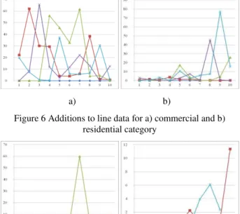
The same tests areas were used to investigate the change in line geometry. Figure 6 illustrates the results of the additions to line geometry. The vertical axis provides the length (in kilometres) of lines added or deleted between epochs and the horizontal axis shows the epochs. Many additions were made in the early days. This could mean that line data was pulled from various sources (including existing data sets) to create the initial base.
Contributions for Cape Town was high in 2007 (epoch 1-2), but decreased thereafter and remained low until early 2010 (epoch 7) However, between late 2010 and early 2011 (epoch 7-8) additions increased significantly. This is significant as epoch 7 is before the 2010 FIFA Soccer World Cup and 8 is immediately after that. In figure 6a additions in Durban had a slow start, but suddenly increased substantially in 2008 (epoch 3-4) and then another big increase between late 2009 and early 2010 (epoch 6-7). Johannesburg also had a significant increase like Durban between late 2007 and early 2008 (epoch 2-3) and then another lower increase between early 2009 and late 2010 (epoch 5-7). Korsten had the lowest volume of increase in additions for the commercial category with two less significant increases between late 2008 and early 2009 (epoch 4-5) and between late 2010 and early 2011 (epoch 8-9).
In Figure 6b additions to residential areas were gradual with a rapid increase for Middleburg in 2010 (epoch 7-8) and also for Universitas between late 2010 and early 2011 (epoch 8-9). Both Brackenfell and Kimberley had very low additions in general, with a minor increase for both areas between late 2008 and early 2009 (epoch 4-5).
a) b)
Figure 6 Additions to line data for a) commercial and b) residential category
a) b)
Figure 7 Deletion to line data for a) commercial and b) residential category
Deletions
Deletions to commercial areas are generally low when compared to the amount of additions made between epochs. In Figure 7a Durban had significantly high deletions between late 2009 and early 2010 (epoch 6-7). In figure 8a it can be seen that during this time period the 2008 data set was modified a lot, as if the entire data set had been shifting in position in 2009. This explains the increase in additions for this period in figure 6a. In Figure 7b deletions to Residential areas are lower than commercial areas, but this can be expected as the total contributions in residential areas are lower than commercial areas. The suburb Universitas also had high deletion values between early 2008 and late 2010 (epoch 6-8). In figure 8b it shows that as with Durban, many modifications were made during this period, accounting for the high deletion values. Brackenfell had high deletion values in 2011 (epoch 9). When examining the data sets, it was noted that an administrative boundary was removed from the early 2011 data set.
a) b)
Figure 8 Difference in position of line data between two datasets: a) Durban – epoch 6-7 and b) Universitas – epoch 6-8
a) b)
Figure 9 Low urban density area: a) additions and b) deletions
Figure 9 represents the additions and deletions for the low urban density category. The line colours represent the low urban density areas as follows: red-Gondeni, green-Makhwezini and purple-Stutterheim. Additions (figure 9a) for low urban density areas were very low when compared to commercial and residential areas. Gondeni had one small addition between late 2010 and early 2011 (epoch 8-9). Makhwezini had two slightly larger additions between late 2009 and late 2010 (epoch 6-8). Stutterheim had one significant increase, when compared to Godeni and Makhwezini, in 2011. Because additions for low urban density areas are low, the deletions are expected to be even lower (figure 9b). Makhwezini and Stutterheim (as with Durban (figure 7a), Brackenfell and Universitas (figure 7b), experienced significant modifications between late 2010 and early 2011 (epoch 8-9) which accounts for relatively high deletion values.
5. DISCUSSION
5.1 Activity
Most line features represented in the test data are either roads or railway lines, Road classes range from national routes to
footways. Single point features are used to represent amenities, e.g. banks, shops, hospitals etc.,
Quantity
OpenStreetMap is first a repository for road data, thus the quantity of line features far exceeds the point features. But it can be expected that with the passage time the acquisition of point features will outstrip that of linear features as these point features are the most likely to change with time.
Quality
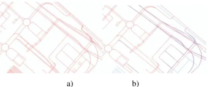
In earlier years, there were much more modifications to line features than in later years. This indicates that the base data is becoming more stable over time.
a) b)
Figure 10 a)Two datasets from 2011 display minor differences. b) The same area compared in 2008 displays many more modifications.
The structure of the OSM database allows for proper classification for both points and lines. This is however not enforced on the user and as a result most of the features are not classified, but only exists on a general field within the database. The result is variation in attribute information for the same features.
5.2 Densification
Rate of mapping
From the results, it becomes clear that the rate of mapping is strongly correlated to the geographical location of an area. Highly populated urban and commercial areas experience greater contributions than towns. This is understandable as such places will contain more people with a culture of sharing information.
Points
The rate of mapping is very different for the three test area categories, from a steady increase for commercial areas, to a much lower rate for residential areas, to no data for low urban areas. The contributions to point features in commercial areas appear to still be increasing.
Lines
In cities and high urban density areas, the quantity of data contributed to OpenStreetMap increased dramatically since 2006. It does however appear that since 2010 very few contributions have been made in these areas. Low urban density areas continue to have a low contribution rate.
5.3 Global vs Local variations
Commercial areas had the highest mapping rate for the 2010-2011 time interval. Residential areas have not had a steady increase in contributions, thus there is no common time period that can be said to have had the most mapping activity.
Commercial areas have had the most additions of line features for the 2007-2009 time intervals. Residential and low urban density areas had the most contributions in 2010-2011.
Considering the time period of this study (six years) it would be expected that low urban density areas would have more contributions. The line features which have been mapped mostly represent the main roads running through the area. These contributions have most likely been made not by the residents but by people passing through.
What should however be taken into consideration is the fact that there is generally not many features to map in these areas, thus high data volumes cannot be expected. Although the residents could provide valuable feature information, the likelihood of this is slim due to the lack of resources.
The contributions to point features in commercial areas appear to still be increasing while the volume of line feature data have had a much higher mapping rate but have stabilised since 2010.
One of the main drivers of a mapping initiative like this is the availability of resources. There exists a digital divide between urban and rural areas. Williams (2001 as cited in Genovese & Roche 2009) describes this as the “gap between people with adequate access to digital information and technology versus those with very limited or no access at all”.
User motivations play a big role in volunteered mapping. Some of these motivations include: “building professional networks”, “strengthening social relationships” (Shekhar 2010) and benefiting others (Coleman et al. 2009). The motivation of an interest group will vary with geographic location and therefore the type of data contributed will vary for different areas. This is seen in the comparison of amenity contributions between commercial and residential areas.
The influx of tourists into an area does have an influence on the number of contributions as can be seen in figure 6, where Cape Town had a surge of contributions leading up to and during the 2010 FIFA Soccer World Cup period. The appreciation that tourists have for a location may have motivated South African citizens to contribute data. On the other hand the tourists themselves could be responsible for the increase in contributions made.
6. CONCLUSION
Haklay & Ellul (2010) conclude that the quality of VGI will vary with the different communities. This study has shown that the rate of mapping and the content of volunteer mapping also vary for different communities . The implication of this is that National Mapping Agencies cannot adopt one standard integration process across the country. VGI is a valuable data source for National Mapping Agencies, thus it would worth developing an integration model that is location specific. How National Mapping Agencies respond to this will have to be addressed in other investigations.
Unlike other forms of information, presently VGI is unlikely to be of a quality as good as National Mapping Agency data. This is not to mean that it is not useful, but rather that our expectations of the data need to be shifted and pragmatic application sought. For example rather than trying to assimilate VGI it can instead be used as a tool to flag blunders in data produced by National Mapping Agencies.
7. Acknowledgements
The authors would like to acknowledge Grant Slater, Muki Haklay from the Department of Civil, Environmental Geomatic Engineering, University of London and Frederick Ramm, managing director of Geofabrik GmbH, Karlsruhe, Germany for providing the OSM test data and information regarding the OSM data.
8. REFERENCES
AL Bakri, M. & Fairbairn, D., 2011. User Generated Content and Formal data Sources for Integrating Geospatial Data. In:
Proceedings of 25th International Cartographic Conference. Paris, France.
Anand, S. et al., 2010. When worlds collide: combining Ordnance Survey and OpenStreetMap data. AGI Geocommunity 10.
Flanagin, A., & Metzger, M., 2008. The credibility of
volunteered geographic information. GeoJournal, 72(3), pp137– 148.
Coleman, D. et al., 2009. Volunteered Geographic Information: The nature and motivation of produsers. International Journal of Spatial Data Infrastructure, 4.
Genovese, E. & Roche, S., 2009. Potential of VGI as a
Resource for SDIs in the North / South Context. Earth, pp.1-15.
Geofabrik, 2011. OpenStreetMap. www.geofabrik.de (5 January 2011).
Girres, J. & Touya, G., 2010. Quality Assessment of the French OpenStreetMap Dataset. Transactions in GIS, 14(4), pp.435-459. Available at: http://doi.wiley.com/10.1111/j.1467-9671.2010.01203 (7 October 2011).
Goodchild, M., 2007. Citizens as sensors: the world of volunteered geography. International Journal of Spatial Data Infrastructure Research, 69(4), 211–221.
Goodchild, M., & Glennon, J., 2010. Crowdsourcing geographic information for disaster response: a research frontier. International Journal of Digital Earth, 3(3), 231–241.
Haklay, M. & Ellul, C., 2010. Completeness in volunteered geographical information the evolution of OpenStreetMap coverage in England (2008- 2009). Journal of Spatial Information Science, 2
Heipke, C., 2010. Crowdsourcing geospatial data. ISPRS Journal of Photogrammetry and Remote Sensing, 65(6), pp 550–557
Shekhar, S., 2010. Contributors of Volunteered Geographic World: Motivation behind Contribution. In: GSDI 12 World Conference. Singapore.
Zielstra, D. & Zipf, A., 2010. A Comparative Study of Proprietary Geodata and Volunteered Geographic Information for Germany, Proceedings of the 13th AGILE International Conference on Geographic Information Science,