Numerical simulation of supersonic gap flow.

(1)

Numerical Simulation of Supersonic Gap Flow

Xu Jing, Huang Haiming*, Huang Guo, Mo Song

Institute of Engineering Mechanics, Beijing Jiaotong University, Beijing, 100044, China

*hmhuang@bjtu.edu.cn

Abstract

Various gaps in the surface of the supersonic aircraft have a significant effect on airflows. In order to predict the effects of attack angle, Mach number and width-to-depth ratio of gap on the local aerodynamic heating environment of supersonic flow, two-dimensional compress-ible Navier-Stokes equations are solved by the finite volume method, where convective flux of space term adopts the Roe format, and discretization of time term is achieved by 5-step Runge-Kutta algorithm. The numerical results reveal that the heat flux ratio is U-shaped dis-tribution on the gap wall and maximum at the windward corner of the gap. The heat flux ratio decreases as the gap depth and Mach number increase, however, it increases as the attack angle increases. In addition, it is important to find that chamfer in the windward corner can effectively reduce gap effect coefficient. The study will be helpful for the design of the ther-mal protection system in reentry vehicles.

Introduction

Thermal protection system (TPS) performance is critical, since mass reduction trades directly with increase in the science payload for a given reentry mass or reduction in launch vehicle cost by using a lighter entry system and a smaller launch vehicle [1]. As is known to all, numer-ous gaps exist in TPS of the supersonic aircraft. For example, TPS of the space shuttle consists of various ceramic insulation tiles. To avoid extrusion damage of ceramic tiles suffering from the heat-expansion and cold-contraction, gaps must be reserved between these tiles. These gaps are able to disrupt the flow field and increase the local heat flux, which could damage the heat shield, and the heat radiation effect in the narrow gaps is blocked, so low heat flux may lead to local overheating. Therefore it is necessary to study the local thermal environment around the gaps under different flight conditions.

Aerodynamic heating flow field around the gap is complex. In recent years, there has been increasing research interesting in the experiment and simulation on the flow field around the gap. A number of previous investigators have considered that empirical and semi-empirical formulas are developed according to experimental data which come from ground and flight tests. For example, Tang [2] from the institute of mechanics Chinese academy of science con-ducted wind tunnel tests of free-stream at Mach numbers of 9.85,12 and 15.5, where heat trans-fer distributions in a gap were measured with a sharp leading edge flat plate and a flat cylinder, and effects of Mach number, attack angle and deflection on heat transfer to the gap wall were discussed. Mori [3] proposed an optical measurement technique for the heat flow onto‘Shaded’

a11111

OPEN ACCESS

Citation:Jing X, Haiming H, Guo H, Song M (2015) Numerical Simulation of Supersonic Gap Flow. PLoS ONE 10(1): e0117012. doi:10.1371/journal. pone.0117012

Academic Editor:Subrata Roy, University of Florida, UNITED STATES

Received:September 19, 2014

Accepted:December 17, 2014

Published:January 30, 2015

Copyright:© 2015 Jing et al. This is an open access article distributed under the terms of theCreative Commons Attribution License, which permits unrestricted use, distribution, and reproduction in any medium, provided the original author and source are credited.

Data Availability Statement:All relevant data are within the paper.

Funding:This work is supported by the National Natural Sciences Foundation of China (No: 11272042, 11472037) and the Project of Education Ministry of China (No:62501036026). The funders had no role in study design, data collection and analysis, decision to publish, or preparation of the manuscript.

(2)

area in the hypersonic flows, in which the present method employs temperature sensitive paint and simple optics installed inside of a model, but the precision of it is still open to dispute. Fur-thermore, in order to redisplay the flow characteristic of high-temperature gas, relatively few studies have considered the simulation on compressible flow. Huanget al[4] applied the vortex method to analyze the supersonic flow. Jackson [5] presented a combined experimental and computational study of laminar cavity flows at hypersonic speeds. Larchevequeet al[6] per-formed large-eddy simulation of the flow over a deep cavity, in which the change of surface pressure, the speed and the noise with time was attained. Hinderkset al[7] investigated hyper-sonic flow with consideration of fluid structure interaction, where the flow field was supposed as laminar flow, and chemical non-equilibrium conditions were adopted in the calculation. Paolicchiet al[8] used the direct simulation Monte Carlo method to do numerical simulation of two-dimensional steady-state hypersonic rarefied flow in a gap at different width-to-depth ratios and wall temperatures. Yanget al[9] developed a hypersonic aero-thermal simulation method for missile flight. Shen et al [10] studied a program of approximate numerical simula-tion of semi-decomposed fluid and solid coupling, and simulated the progress of a high speed airflow impacting the seal structure. However, the data are still scarce, and we need to provide more records, so further numerical simulations on the flow around a gap are still essential work at present.

In this study, two-dimensional compressible Navier-Stokes equations are solved by the fi-nite volume method to obtain the local aerodynamic heating environment around a gap.

Models

Physical Models

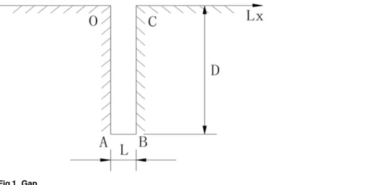
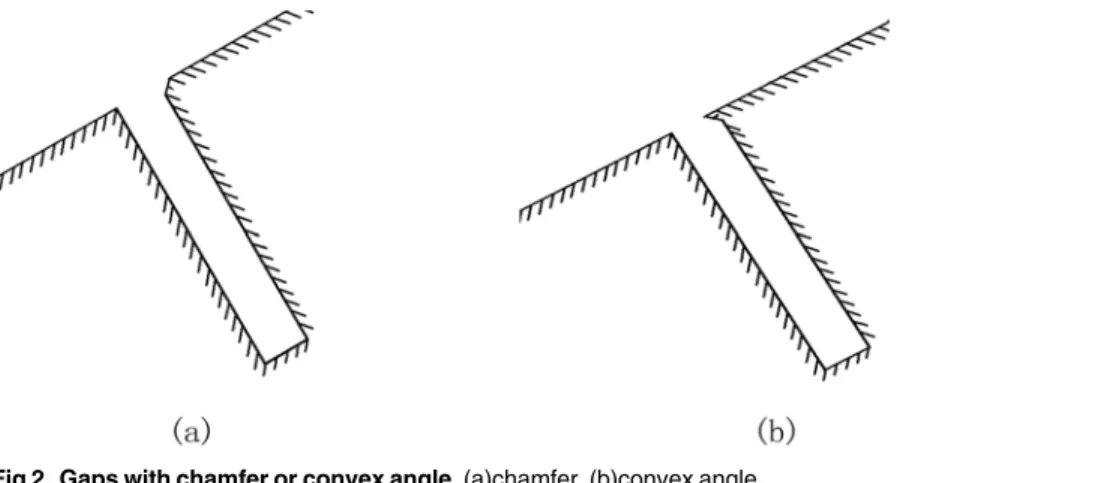
As can be seen inFig. 1, Lx is the coordinate along the wall and its positive direction is from O to A to B to C. Firstly, when width (L)-to-depth (D) ratio L/D = 1/6, numerical models under different conditions—attack angle (α) = 0°,15° and 30°—are performed separately to analyze the influence of attack angle on the flow around a gap. Secondly, we hope to know the influence of width-to-depth ratio on gap effect, so models of L/D = 1/2 and 1/4 are built while width L re-mains 2 mm. Thirdly, chamfer and convex angles are seen inFig. 2(a) and (b)in order to ana-lyze the influence of chamfer and convex angle whenα= 30° and L/D = 1/6. The length of the chamfer inFig. 2(a)in slope direction x = 0.5mm and the length along the gap windward side

Fig 1. Gap.

(3)

y = 0.5mm. InFig. 2(b), the length of the convex angle in slope direction x = 0.5mm and the length along the gap windward side y = 0.5mm.

InFig. 3(a), in order to match far field boundary condition, the distance between corner point G and left pressure far field boundary is 120mm, so does the distance between point G and top pressure far field boundary, while that between point G and right pressure far field boundary is 140mm. The projection of the slope in the horizontal direction is 40mm long. The various gaps above may be located in the middle of the slope. In addition, in order to study the effect of different parameter on gap local aerodynamic heating environment, smooth plate models without gaps are also built and the other sizes are as same as that inFig. 3(a).

Define deflection angleβas the angle between the flow direction and the vertical direction of gaps inFig. 3(b). If the deflection angleβis not equal to zero, the three-dimensional effects should be considered. But in this paper, the simulation needs to be done under the condition that the deflection angleβis equal to zero.

Mathematical Model

Based on the physical model above, the two-dimensional mathematical model can be estab-lished. Governing equations for the turbulent flow around a gap are described by the Fig 2. Gaps with chamfer or convex angle.(a)chamfer, (b)convex angle.

doi:10.1371/journal.pone.0117012.g002

Fig 3. Relation between a flow and a gap.(a) Physical model, (b) Vertical view of a gap.

(4)

differential equations

@r @tþ

@ @xi

ðruiÞ ¼0 ð1Þ

@

@tðruiÞ þ

@ @xj

ðruiujÞ ¼

@P

@xi

þ @

@xj

ðm@ui

@xj

ru0

iu0jÞ ð2Þ

@ @tðrTÞ þ

@ @xj

ðrujTÞ ¼

@ @xj

ðk c

@T

@xj

ru0

iT0Þ ð3Þ

Whereu1,ρ,P,T,µ,k,care the velocity component, density, pressure, temperature, viscosity

coefficient, thermal conduct coefficient and specific heat capacity offluid, respectively;i= 1,2; j = 1,2; Roe discrete format is adopted in the discretization of the convection term, and 5-step Runge-Kutta algorithm is used in discretization of time term.

In the above equations, S-A turbulence model is adopted on the base of Boussinesq hypoth-esis [11], in which turbulence variablemis introduced, so turbulent viscosityµtis given in the

form

m_t¼mfv1 ð4Þ

whereƒ_v1=X3/(X3+Cv1),w¼m=m, and turbulence variablemcan be deduced as

@m @t þ

@ðmuiÞ

@xj

¼ fr½ðmþmþCb2mÞrm Cb2mD mg=sþQ ð5Þ

whereσandCb2are constantsQis the source term in the form

Q¼Cb1Sm Cw1fwðm=dÞ 2

ð6Þ

SSfv3þmfv2=ðk 2

d2_Þ _ð

7Þ

S ffiffiffiffiffiffiffiffiffiffiffi2SijSij

q

ð8Þ

Sij¼ ð

@uj

@xi

@ui

@xj

Þ=2 ð9Þ

fv2 ¼ ð1þw=Cv2Þ 3

ð10Þ

fv3¼ ð1þwfv1Þð1 fv2Þ=w ð11Þ

fw¼g½ð1þC 6 w3Þ=ðg

6_þ

C6 w2Þ

1=6

ð12Þ

g ¼rþCw2ðr 6

rÞ;r¼m=ð_Sk2

d2_Þ _ð

13Þ

Cw1 ¼Cb1=k

2_{þ ð}₁_þ_C

b2Þ=s ð14Þ

wheredis the distance to the wall surface, others are seen inTable 1.

(5)

Computational Conditions

Both inside and outside surfaces of the gap are not slip wall or cold wall. The wall is set for an isothermal wall condition of 300K. The flow field is initialized by uniform flow which has the same inflow velocity. The initial air temperature is also 300K. The entrance, exit and the upper boundary are supposed to be pressure far fields boundary condition. The far field pressure equals to standard atmospheric pressure. In addition, The Mach numbers of free steam are 2, 3 and 4, respectively.

Constant-pressure specific heatCp= 1006.43J/kgK and heat conduction coefficient equal to

0.0242W/mK. The viscosity of flow can be determined by Sutherland Law

m m₀ ¼

T T0

1:5

T0þTS

TþTS

Whereµis the air viscosity corresponding toT, whileµ0is the reference viscosity

corresponding to a reference temperatureT0= 231K,TSis the Sutherland constant 110K, and

µ0= 1.716 × 10-5.

Computational Grids

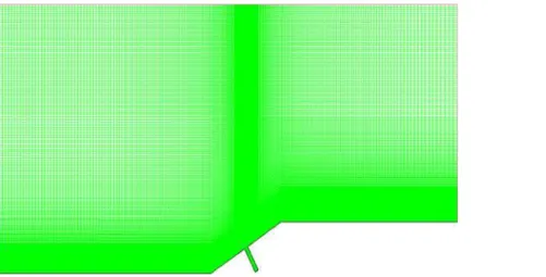
To get more accurate results, the grid is denser near the wall and in the gap. The sum of grids is approximately 230,000, and 70×270 grids in the gap. The distance between the nearest bound-ary layer grids and wall is 5×10-6m to guarantee the accuracy of calculation.Fig. 4is the computational grid whenα= 30° and L/D = 1/6. Moreover, there are 70×110 grids in the gap when L/D = 1/2, and 70×190 grids in the gap when L/D = 1/4. Grids outside the gap are as same as L/D = 1/6.

Note that dense triangle grid is employed in chamfer area and convex angle area. Different mesh densities were analyzed in a previous study and there was thin difference. The dense structural grid adopted in the paper is stable.

Table 1. Model Parameters.

Cw2 Cw3 Cv1 Cv2 Cb1 Cb2 k σ

0.3 2 7.1 5 0.1355 0.622 0.41 2/3

doi:10.1371/journal.pone.0117012.t001

Fig 4. Computational grids (α= 30° and L/D = 1/6).

(6)

Results

Effect of Mach number on Gap Effect

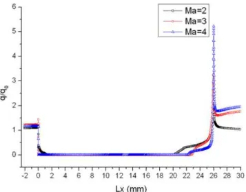
The ratio of gap heat fluxqto the smooth plate heat fluxq0in the corresponding location is de-fined as the heat flux ratio. As are shown in Figs.5,6and7, curves of heat flux ratio in different conditions (L/D = 1/6,α= 0°,15°,30° and Ma = 2,3,4) can be gained by calculating the corre-spondingqandq0.

The heat flux ratio is basically U-shaped distribution along the surface of a gap. Owing to the impaction of high-speed flow onto windward of gap, heat flux ratio on windward is larger than that on leeward. The speed of flow at the bottom of the gap is almost 0, so the ratio is close to 0. Heat flux ratio in the gap decreases as Mach number increases, because the boundary layer tends to be thinner and air flowing into the gap decreases as Mach number increases.

Fig 5. Distribution of heat flux ratio along the gap with L/D = 1/6 whenα= 0°.

Fig 6. Distribution of heat flux ratio along the gap with L/D = 1/6 whenα= 15°.

(7)

In order to validate the reliability of the numerical simulation method mentioned in the paper, the result has been compared with one of supersonic velocity wind tunnel experiment, in which the data of the experiment came from reference [12]. The comparison of the heat flux ratio between numerical simulation and experiment (Ma = 5) whenα= 0° is shown inFig. 5. The simulation results match well with the experiment.

Effect of Attack Angle on Gap Effect

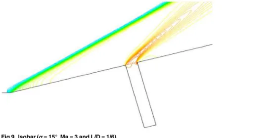
Isobar under condition thatα= 0°,15°,30° and Ma = 3 is shown in Figs.8,9and10. Pressure in-side the gap is almost constant regardless of the attack angle, which shows that the flow speed must be low in the gap.

Figs.11,12and13present the isodensity lines under condition thatα= 0°,15°,30° and Ma = 4. Whenα= 0°, the disturbance region of outflow only exists in the upper portion of

gaps, which shows that the mass flow rate of outflow into gaps is little. The disturbance region Fig 7. Distribution of heat flux ratio along the gap with L/D = 1/6 whenα= 30°.

Fig 8. Isobar (α= 0°, Ma = 3 and L/D = 1/6).

(8)

is increasing, but is still a partial volume of the gap whenα= 15°. However, whenα= 30°, the

disturbance region expands to the whole gaps.

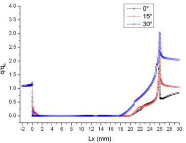
Distributions of heat flux ratio in different conditions are reported in Figs.14,15and16. The heat flux at the bottom of the gap is almost zero and the curve of the heat flux ratio almost keeps horizontal as attack angle changes. However, the effect of attack angle on heat flux on the upper part of windward is obvious. The heat flux ratio increases in the upper area with the in-crease of attack angle, because the air flowing into the gap inin-creases as attack angle inin-creases.

Effect of Width-to-depth Ratio on Gap Effect

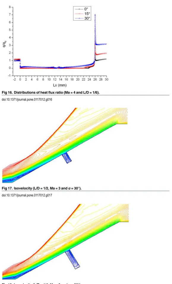
Isovelocity under condition that L/D = 1/2,1/4,1/6, Ma = 3 andα= 30° is given in Figs.17,18 and19. The isovelocity occupies the whole gap area inFig. 17. InFig. 18it just occupies most part of the area and the speed of flow at the bottom part of the gap is quite low. InFig. 19the flow speed at most part of the gap keeps zero. As the depth of gap increases, the flow speed decreases.

Fig 9. Isobar (α= 15°, Ma = 3 and L/D = 1/6).

Fig 10. Isobar (α_{= 30°, Ma = 3 and L/D = 1/6).}

(9)

Fig 11. Isodensity pattern (α= 0°, Ma = 4 and L/D = 1/6).

(10)

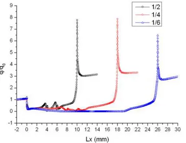
Distribution of heat flux ratio under condition that L/D = 1/2,1/4 or 1/6, Ma = 3 andα= 30° is shown inFig. 20. It is obvious that the heat flux ratio at the bottom of the gap decreases as the width-to-depth ratio of the gap decreases. In Figs.17and18the flow speed at the bottom is not zero, but that inFig. 19is zero. The heat flux ratio is greater than zero at L/D = 1/2 or 1/4, but that keeps almost zero at L/D = 1/6.

Gap Effect Coefficient

It is known that heat flux ratio always peaks at turning point of windward surface of the gap. The maximum of heat flux ratio is defined as the gap effect coefficient, which is used to repre-sent degree of the gap effect in aerodynamic heating.

Distribution of gap effect coefficient under the condition that Ma = 2,3,4 andα= 0°,15°,30° is seen inFig. 21. It can be seen fromFig. 21that the gap effect coefficient increases with the in-crease of Mach number and attack angle.

Fig 14. Distributions of heat flux ratio (Ma = 2 and L/D = 1/6).

(11)

Fig 17. Isovelocity (L/D = 1/2, Ma = 3 andα= 30°).

(12)

In order to reduce the gap effect coefficient, chamfer and convex angle are set in the wind-ward. Isodensity patterns (convex angle with x = y = 0.5mm, chamfer with x = y = 0.5mm or x = 1mm, y = 0.5mm) when Ma = 4 andα= 30° are described inFig. 22(a), (b) and (c). Com-paringFig. 22(a) and (b)withFig. 22(c), it is obvious that the effect of external flow with cham-fer on gap only occurs in the open area of the gap. Part of high temperature air which could flow into gap through the chamfer, so the heat flux in gaps reduces effectively because of the chamfer.

ComparingFig. 22(a)withFig. 22(b), as the length x of the chamfer in slope direction in-creases from 0.5mm to 1mm and length y along the gap windward side is 0.5mm, the effect of small angle chamfer on incoming flow decreases. The isodensity lines of the model with convex Fig 19. Isovelocity (L/D = 1/6, Ma = 3 andα= 30°).

Fig 20. Distribution of heat flux ratio (Ma = 3 andα= 30°).

(13)

angle are shown inFig. 22(c). Owing to the existence of convex angle, external flow reaches the bottom of the gap.

Distributions of heat flux ratio of two models with chamfer under condition that Ma = 4 andα= 30° are shown inFig. 23andFig. 24, respectively. It can be seen fromFig. 23and Fig. 24that the distribution of heat flux ratio along the surface of gap with chamfer is still U-shaped curve and except the opening area the heat flux ratio at most part of the gap almost equals to zero.

Compared with gap effect coefficient 7.028 inFig. 7(α= 30°, Ma = 4 without chamfer), it decreases to 1.358 when setting chamfer shown inFig. 23, and to 1.78 inFig. 24. Both gap effect coefficients are gained at the peak of the chamfer. Thus, setting chamfer in the windward can reduce the gap effect coefficient, which is a valid method for reducing the gap local aerodynam-ic heating environment.

Fig 21. Distribution of gap effect coefficient (L/D = 1/6).

Fig 22. Isodensity pattern of model with chamfer and convex angle (L/D = 1/6).(a)chamfer(x = y = 0.5mm), (b)chamfer(x = 1mm, y = 0.5mm), (c)convex angle(x = y = 0.5mm).

(14)

As shown inFig. 25, gap effect coefficient goes up to 7.7945, compared with 7.028 without convex angle. A convex angle aggravates the aerodynamic heating in the gap. In order to pre-vent structure from failure, convex angle should be avoided in the design of engineering struc-ture suffering from airflow at high temperastruc-ture.

Conclusions

Numerical simulation of two-dimensional flow around a gap is accomplished using the finite volume method. From the numerical results, it can be concluded as follows:

a) The heating ratio along the Lx coordinate in gaps shows‘U’curve approximately, the peak value appears at the corner of the windward surface of gaps because of the subsequent Fig 23. Distribution of gap heat flux ratio.(L/D = 1/6, Ma = 3,α= 30° and chamfer(x = y = 0.5mm))

Fig 24. Distribution of gap heat flux ratio.(L/D = 1/6, Ma = 3,α= 30°and chamfer (x = 1mm, y = 0.5 mm))

(15)

shock wave, and the gap effect depends not only on the attack angle, but also on the Mach number.

b) Chamfer in the windward corner can effectively reduce gap effect coefficient, whereas the convex angle would increase gap effect coefficient.

Author Contributions

Conceived and designed the experiments: XJ HH HG MS. Performed the experiments: XJ HG MS. Analyzed the data: XJ HG MS. Wrote the paper: XJ HH HG MS.

References

1. Huang HM, Li WJ, Hu HL (2014) Thermal analysis of charring materials based on pyrolysis interface model. Thermal Science, 2014, 18(5):1583–1588.

2. Tang GM (2000) Experimental investigation of heat transfer distributions in a deep gap. Experiments and Measurements in Fluid Mechanics 14(04): 1–6.

3. Mori K (2012) Optical measurement of heat-flux onto‘Shaded’area in hypersonic flows (I): Preliminary measurement of heat-flux in a deep cavity. 43rd, AIAA, Thermophysics Conference, New Orleans, Louisiana, June 25–28.

4. Huang HM, Huang G, Xu XL, Li WJ (2014) Simulation of co-rotating vortices based on compressible vortex method. International Journal of Numerical Methods for Heat and Fluid Flow, 2014, 24 (6):1290–1300.

5. Jackson AP, Hillier R, Soltani S (2001) Experimental and computational study of laminar cavity flows at hypersonic speeds. Journal of Fluid Mechanics 427: 329–358. doi:10.1017/S0022112000002433

6. Larcheveque L, Sagaut P, Le T, Comte P (2004) Large-eddy simulation of a compressible flow in a three-dimensional open cavity at high Reynolds number. Journal of Fluid Mechanics 516: 265–301. doi:10.1017/S0022112004000709

7. Hinderks M, Radespiel R (2006) Investigation of hypersonic gap flow of a reentry nosecap with consid-eration of fluid structure interaction. 44th, AIAA, Aerospace Sciences Meeting and Exhibit, Reno, Ne-vada, Jan. 9–12.

8. Paolicchi L, Santos W (2010) Suface temperature impact on the aerodynamic suface quantities of hy-personic gap flow. National Congress of Mechanical Engineering, Campina Grande—Paraíba—Brazil, Aug. 18–21.

9. Yang K, Gao XW (2012) Aeroheating CFD analysis of missile slots. Theoretical and Applied Mechanics Letters. 2(1): 012003–3. doi:10.1063/2.1201203

Fig 25. Distribution of gap heat flux ratio.(L/D = 1/6, Ma = 3,α= 30° and convex angle(x = y = 0.5 mm))

(16)

10. Shen C, Xia XL, Cao ZW, Yu MX (2012) Analysis of mass flow and heat-transfer characteristic of the gap-cavity sealing structure under the impact of high-speed airflow. Acta Aeronautica et Astronautica Sinica. 33(1):34–43.

11. Spalar PR, Allmaras SR (1992) A one-equation turbulence model for aerodynamics flows. 30th, AIAA, Aerospace Science Meeting and Exhibit, Reno, Nevada, Jan. 6–9.