Connectivity Patterns in fMRI Data of the Human Brain
Gabriele Lohmann1*, Daniel S. Margulies1, Annette Horstmann1, Burkhard Pleger1, Joeran Lepsien1, Dirk Goldhahn1, Haiko Schloegl2, Michael Stumvoll2, Arno Villringer1, Robert Turner1
1Max Planck Institute for Human Cognitive and Brain Sciences, Leipzig, Germany,2Department of Medicine, University of Leipzig, Leipzig, Germany
Abstract
Functional magnetic resonance data acquired in a task-absent condition (‘‘resting state’’) require new data analysis techniques that do not depend on an activation model. In this work, we introduce an alternative assumption- and parameter-free method based on a particular form of node centrality called eigenvector centrality. Eigenvector centrality attributes a value to each voxel in the brain such that a voxel receives a large value if it is strongly correlated with many other nodes that are themselves central within the network. Google’s PageRank algorithm is a variant of eigenvector centrality. Thus far, other centrality measures - in particular ‘‘betweenness centrality’’ - have been applied to fMRI data using a pre-selected set of nodes consisting of several hundred elements. Eigenvector centrality is computationally much more efficient than betweenness centrality and does not require thresholding of similarity values so that it can be applied to thousands of voxels in a region of interest covering the entire cerebrum which would have been infeasible using betweenness centrality. Eigenvector centrality can be used on a variety of different similarity metrics. Here, we present applications based on linear correlations and on spectral coherences between fMRI times series. This latter approach allows us to draw conclusions of connectivity patterns in different spectral bands. We apply this method to fMRI data in task-absent conditions where subjects were in states of hunger or satiety. We show that eigenvector centrality is modulated by the state that the subjects were in. Our analyses demonstrate that eigenvector centrality is a computationally efficient tool for capturing intrinsic neural architecture on a voxel-wise level.
Citation:Lohmann G, Margulies DS, Horstmann A, Pleger B, Lepsien J, et al. (2010) Eigenvector Centrality Mapping for Analyzing Connectivity Patterns in fMRI Data of the Human Brain. PLoS ONE 5(4): e10232. doi:10.1371/journal.pone.0010232
Editor:Olaf Sporns, Indiana University, United States of America
ReceivedNovember 6, 2009;AcceptedMarch 22, 2010;PublishedApril 27, 2010
Copyright:ß2010 Lohmann et al. This is an open-access article distributed under the terms of the Creative Commons Attribution License, which permits unrestricted use, distribution, and reproduction in any medium, provided the original author and source are credited.
Funding:This work was supported by the Bundesministerium Bildung und Forschung (BMBF), http://www.bmbf.de/, Foerderkennzeichen: 01GI0850, Projekt-Nr.: 934000-391; and the European Union’s Seventh Framework Programme (Grant No. 223057). The funders had no role in study design, data collection and analysis, decision to publish, or preparation of the manuscript.
Competing Interests:The authors have declared that no competing interests exist. * E-mail: [email protected]
Introduction
Functional magnetic resonance data (fMRI) of the human brain acquired in a task-absent (‘‘resting state’’) condition has attracted increasing interest in recent years. Due to the absence of an experimental paradigm, analysis procedures based on an activa-tion model are not applicable. New types of techniques have been developed focusing on functional connectivity rather than task activation. For instance, correlation of time series between a pre-specified seed region and all other voxels of the brain is robust and conceptually clear. However, it can only be successfully applied if some prior knowledge exists for identifying seed regions. Another widely used technique is based on independent component analysis (ICA) whose primary advantage is its freedom from hypotheses preceding the analysis and the need for selecting seed regions [1]. However, the number of independent components is difficult to specify and assumptions must be made about what constitutes a valid network. For comprehensive reviews of the above and related methods see [2,3].
More recently however, graph-based methods have been proposed for the analysis of functional and structural magnetic resonance data of the human brain. Their main feature is that they take brain regions as nodes in a graph. Some of these methods have also been applied to the analysis of resting state fMRI data [4–6]. Given the small world
properties of the human brain [7,8], graph-based methods provide a valuable tool for elucidating network structures.
In the present study, we focus on a particular type of graph-based method that identifies nodes which play central roles within the network structure. Such nodes are characterized by a measure called ‘‘node centrality’’. Node centrality is a key concept in social network analysis of which several competing definitions exist and some of which have been applied to fMRI data analysis in the past [5,9]. Here we discuss several of these approaches - in particular ‘‘betweenness centrality’’, ‘‘degree centrality’’ and ‘‘eigenvector centrality’’. Sporns et al. [9] for instance advocate a combination of various graph measures including degree, betweenness centrality and closeness centrality.
Thus far, centrality measures have been applied to a pre-selected set of nodes consisting of at most several hundred elements (e.g. [6,8,9]). Here, we propose to apply this measure to all voxels in a region of interest covering the entire cerebrum thereby avoiding any selection bias [10].
weights nodes based on their degree of connection within the network. It does so by counting both the number and the quality of connections so that a node with few connections to some high-ranking other nodes may outrank one with a larger number of mediocre contacts [13]. Google’s ‘‘PageRank’’ algorithm is a variant of eigenvector centrality [14]. Both the human brain and the world wide web exhibit small world properties suggesting that an algorithm that is effective as part of a search engine may also be effective in analyzing network properties of the human brain.
Eigenvector centrality can be used on a variety of different similarity metrics. Here, we present applications based on linear correlations and on spectral coherences between times series. This latter approach allows us to draw conclusions about connectivity patterns in different spectral bands. The motivation for choosing spectral measures came from Salvador et al. [15] who have emphasized the importance of investigating interregional depen-dencies in the frequency domain rather than in the time domain. We propose to use eigenvector centrality as a mapping tool for the entire brain or parts of it. Such maps can be subjected to statistical tests to detect groupwise differences in centrality between experimental states. For abbreviation, we will call this method ECM (Eigenvector Centrality Mapping).
Materials and Methods
Several definitions of node centrality exist - each having a slightly different interpretation. Common to all of these definitions is that they are based on a symmetric matrix containing pairwise similarity measures. LetAbe such ann|nsimilarity matrix where entries aij,i,j~1,:::n contain a pairwise similarity measure
between time series in voxelsiandj. The number of voxelsnis determined by user-specified regions of interest (ROI) to which all subsequent analysis steps are restricted. In the experiments reported in this study, the ROI covered the entire brain excluding the cerebellum and consisted ofn&40,000voxels.
The matrixAis symmetric so that each voxel can be viewed as a node in an undirected weighted graph in which similarity values correspond to weights along the edges of the graph. In graph-based applications, these weights represent distances between nodes and are therefore non-negative. As a result, centrality measures are generally also defined to be non-negative. See Bonacich [16] for a discussion of this point.
Degree centrality
The simplest centrality measure is called ‘‘degree centrality’’. The degreexiof a nodeiis defined as
xi~
X
j
aij:
Thus, a node has a high degree if it has strong connections to many other nodes in the graph.
Eigenvector centrality
Eigenvector centrality was first introduced by Bonacich [11,12] and a later variant of it is a central part of Google’s PageRank algorithm [14]. Much like degree centrality, it favours nodes that have high correlations with many other nodes. However, in contrast to degree centrality it specifically favours nodes that are connected to nodes that are themselves central within the network. Thus it takes into account the entire pattern of the network.
As before let A denote an n|n similarity matrix. Then the eigenvector centralityxiof nodeiis defined as thei-th entry in the
normalized eigenvector belonging to the largest eigenvalue ofA.
Note that with this definitionxifulfils the characteristics described
above. To see why let l be the largest eigenvalue and x the corresponding eigenvector, then
Ax~lxor equivalently,x~1
lAx, andxi~m Xn
j~1 aijxj
with proportionality factorm~1=lso thatxiis proportional to the
sum of similarity scores of all nodes connected to it.
Uniqueness of this definition is ensured by the Perron-Frobenius theorem which states that any square matrix with strictly positive entries has a unique largest real eigenvalue with strictly positive components. This is also true for irreducible square matrices with negative entries. An irreducible matrix has at least one non-zero off-diagonal element in each row and column.
Since we assume thatArepresents distances between nodes we haveaij§0,Vi,j. In the present context, we may assume thatAis
irreducible because fMRI time series are almost never entirely dissimilar so that a sufficient number of non-zero entries inAexist. Thus, an eigenvector belonging to the normalized largest eigenvalue exists and its entries xi provide a centrality measure
for each nodeiwhich is uniquely defined and non-negative. Note that symmetric matrices with negative entries may have several largest eigenvalues that are not distinct so that the requirement of non-negativity is essential for ensuring the uniqueness of this definition (see Appendix S1 for an example).
Eigenvector centrality is related to principal components analysis (PCA) in that both methods are based on eigenvector decompositions of similarity matrices. However, PCA differs from eigenvector centrality in that it only allows linear correlations as a similarity metric. But linear correlations may be negative so that the first principal component is not uniquely defined because of possible multiplicities of eigenvalues.
In our experiments we used linear correlations which were re-scaled to be non-negative and also a spectral coherence metric which is non-negative by definition (see below). Other similarity metrics such as mutual information or wavelet transform coherence (WTC) [17] might be used for eigenvector centrality mapping (ECM) as well.
Many algorithms for computing eigenvectors of symmetric matrices are known. In the present context, it suffices to find the eigenvector belonging to the largest eigenvalue. For this special case, the power iteration method [18, 405ff] is one of the most efficient, and was used in our experiments.
Betweenness centrality
The betweenness centralityxiof some nodeiis defined as:
xi~
X
i=j,i=k j=k
sjk(i)
sjk
wheresjkis the number of shortest geodesic paths fromjtok, and
sjk(i)is the number of shortest geodesic paths fromjtokthat pass
analyzing spontaneous fluctuations in a network consisting of 90 regions of interest. We tested betweenness centrality on a region of interest containing 17,398 voxels that covered parts of the left hemisphere of one subject. The computation took 26 hours using 4 parallel 2.6 GHz processors for a single data set. Application to a region of interest with full brain coverage was not feasible.
Linear correlation
Linear correlation has been proposed as a metric for analysing functional connectivity [20]. A high positive correlation between two fMRI time series indicates a strong similarity, a high negative a strong dissimilarity. Note that this measure is quite agnostic about any form of causal influence between brain regions. It is defined as follows.
Letxi,i~1,:::,Nandyi,i~1,:::,Nbe time series of lengthNin
two voxelsxandy. Their correlation is defined as
r~
PN
i~1(xi{x)(yi{y)
(N{1)sxsy
where x,y denote the sample mean and sx,sy the standard
deviations.
Because the similarity matrix A should be positive, linear correlations between time series must be re-scaled accordingly. We propose to use
~rr~rz1
whererdenotes the correlation between two time series and~rrthe corresponding scaled version. Note however that strong negative correlations may indicate some form of inverse coupling. Therefore, an alternative way to handle negative correlations might be to take absolute values instead of the approach proposed here.
Spectral coherence
Salvador et al. [15] have noted that interregional dependencies can be more readily observed in the frequency domain than in the time domain. Therefore, we have also used frequency based similarity metrics for ECM. Specifically, we employ spectral coherence for this purpose. It has been previously applied to fMRI data analysis [15,21,22]. In the following, we give a brief overview. For more information see for instance [23,24].
Let Xt,Yt denote real-valued stationary time series in two
voxels, and letvbe some frequency of interest. We assume that they are normalized to zero mean. Their cross-correlation function evaluated at lagkis defined as
CSXY(k)~E(XtzkYt)
and the corresponding cross-spectral density is:
fXY(v)~
X
k
W(k)CXY(k) exp ({2pivk)
Analogously, the auto-spectral density of a single time courseXis
fX(v)~
X
k
W(k)CXX(k) exp ({2pivk)
Several choices for the weighting factorsW(k) exist. Among the most common ones are Parzen or Tukey windows. Here, we used
the Tukey window which is defined as:
W kð Þ~ 1 2 1zcos
pk m
forDkDƒm
0 otherwise
8 <
:
wheremis the number of lags to compute the autocorrelation for. As a rule of thumb, m should be chosen to be in the range N=20vmvN=3 where N is the length of the time series [25, p.141]. In the data presented below the time series length was N~168, and we usedm~10throughout.
SinceCSxy(v)is not necessarily symmetric the cross-spectrum
is generally a complex function. The real part offXY(v)is known
as the cospectrum denoted ascsXY(v)and the imaginary part as
the quadrature spectrum qsXY(v). The spectral coherence
yXY(v)betweenX,Y at frequencyvis defined as:
yXY(v)~
ffiffiffiffiffiffiffiffiffiffiffiffiffiffiffiffiffiffiffiffiffiffiffiffiffiffiffiffiffiffiffiffiffiffiffiffiffiffiffiffiffiffiffiffi qsXY(v)2zcsXY(v)2
fX(v)fY(v)
s
[½0,1
Note that information about phase lags is not included in the above measure. Frequency-dependent phase coherence can be computed using the above definitions as follows
phaseXY(v)~arctan
csXY(v)
qsXY(v)
:
Experiment 1
Functional MRI/EPI data were acquired of 35 normal volunteers on a 3T MRI scanner (Siemens Tim Trio) using TR = 2.3 sec, TE = 30ms, 363 mm2 in-plane resolution, 3 mm slice thickness, 1 mm gap between slices. Each scanning session began with a task-absent (‘‘resting state’’) scan lasting 7.6 minutes during which subjects were asked to fixate a fixation cross. A second resting state scan with the same acquisition parameters followed about 10 minutes later within the same scanning session. In between these two scans, subjects were scanned in another task absent condition using sagittal instead of axial slices. Data from this scan were not used for the present study.
All data sets were initially fieldmap corrected using the software system Lipsia [26]. Data preprocessing then continued using FSL [27], and consisted of motion correction, bandpass filtering (SPECS), and spatial smoothing (SPECS). Finally, preprocessed data sets were registered into standard MNI152 (Montreal Neurological Institute) brain space using FSL’s nonlinear registra-tion software FNIRT, and resampled to an isotropic voxel grid with a resolution of 36363 mm3. We manually defined a region of interest containing about 52,000 voxels covering the entire cerebrum to which subsequent ECM analysis was applied (Figure 1).
Experiment 2
we first acquired resting state data for 6.5 minutes during which subjects were asked to fixate a fixation cross. During the following 34 minutes they were shown pictures of food and tools that they were asked to respond to by button presses. Finally, another 6.5 minutes of resting state data were acquired. In the present study, we only analyzed the initial resting state data acquired before visual stimulation began, and ignored the rest of the experiment.
Data processing was done using the software system Lipsia [26]. All data sets were initially corrected for motion and slicetime offsets. A baseline correction was applied using a highpass filter with a cutoff frequency of 1/90 Hz, and a spatial smoothing with a Gaussian filter of fwhm = 8 mm was used. All data sets were initially registered to an AC/PC coordinate system where the data were resampled to an isotropic voxel grid with a resolution of 36363mm3. We manually defined a mask containing
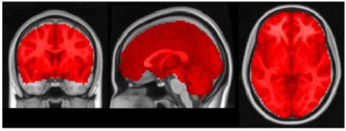
&40,000 voxels covering the entire brain while excluding the cerebellum and parts of CSF (Figure 2).
Data processing
For both experiments, we computed pairwise similarity matrices between time series of any two voxels inside the mask using scaled linear correlation and for experiment 2 also spectral coherence, and applied the ECM algorithm to these matrices. The resulting centrality maps were then transformed as described by van Albada et al. [28] in order to ensure that they obey a Gaussian normal distribution as required for subsequent statistical tests. The results were corrected for multiple comparisons using cluster-size and cluster-value thresholds obtained by Monte-Carlo simulations [29,30] using a significance level of pv0:05. Clusters in the resulting maps were obtained using an initial z-value threshold of 2.33. The Monte Carlo simulation determines the size and peak value a cluster must have in order to be considered statistically significant. Thus, a cluster with only a moderately high peak value
might be considered significant if it is large enough. On the other hand, a cluster with a very high peak value might be significant even if it is rather small. Computation times for ECM were about 20 minutes per dataset on a 2.6 GHz Opteron processor. About 6 GByte of computer memory are needed to store ann|nmatrix with n~40,000 voxels to cover the cerebrum at 3|3|3mm3 resolution.
Results
Experiment 1
Figure 3 shows group averages of eigenvector centrality in the two scans. A network of hubs including sensorimotor areas of the marginal ramus of the cingulate and mid-cingulate, thalamus, primary visual cortex, insula and operculum are common to both. Figure 4 shows results of a paired t-test contrasting the two scans. During the first scan, eigenvector centrality scores were signifi-cantly higher in left and right thalamus and in the cerebellum. During the second scan, eigenvector centrality was larger in posterior cingulate, medial frontal and right opercular cortices, and medial frontal areas.
For comparison, we additionally computed another centrality map - this time using degree centrality instead of eigenvector centrality (Figure 5). Note that during the second scan, degree centrality was larger almost everywhere in the brain.
Experiment 2
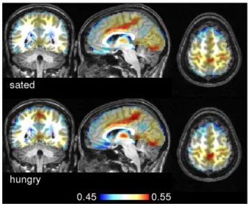
Figure 6 shows group averages of ECM based on scaled linear correlation. The overall ECM pattern looked very similar although we found statistically significant differences in precuneus when contrasting hungry against sated state (Figure 7 and Appendix S2). Recent literature postulated that posterior midline cortex, comprising precuneus and posterior cingulate cortex constitutes the core hub within the default network of the human brain with strong connections to ventral medial prefrontal cortex/ anterior cingulate cortex, inferior lateral parietal cortex, and the hippocampi [31,32]. This particular portion of the precuneus, located in the anterior section adjacent to the marginal ramus of
Figure 2. The region of interest in experiment 2.The mask used in experiment 2 containing about &40,000voxels. Talairach coordi-nates of slice positions are (0,0,0).
doi:10.1371/journal.pone.0010232.g002
Figure 3. Group averages of eigenvector centrality maps in experiment 1.The group average of the first scan is shown in the top row. The bottom row shows results of the second scan. The similarity metric was scaled linear correlation. MNI coordinates of slice positions are (24,271,220).
doi:10.1371/journal.pone.0010232.g003 Figure 1. The region of interest in experiment 1. The mask
the cingulate sulcus, has been implicated in self-related processing (in contrast to the episodic memory-related role of the posterior precuneus) [33]. Although the enhanced centrality of precuneus during the hungry state indicates a changed core hub of the default network, we found no other areas with significantly changed centrality values across the brain. Nonetheless, the increased centrality of anterior precuneus during the hungry state is consistent with the proposed self-related functionality of this region.
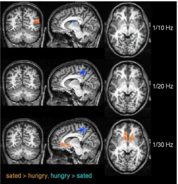
We next employed spectral coherence to investigate frequency based similarity metrics because of their known advantages in the observation of interregional dependencies [15]. We found strong effects of frequency in ECM across spectral bands as shown in Figure 8. In frequency bands 1/10 Hz up to 1/20 Hz, ECM was significantly larger in precuneus, the striatum and several more areas. Very low frequency bands (1/25 Hz, 1/30 Hz, 1/35 Hz) dominate at the temporal poles and mediodorsal frontal areas.
Figure 9 and Table 1 show differences between the sated and the hungry state across various spectral bands based on spectral coherence. In particular, differences appear in the anterior precuneus at 1/20 Hz and 1/30 Hz, and in the ventral striatum at 1/30 Hz.
Discussion
We propose eigenvector centrality as a new method for analyzing fMRI data. It is parameter-free, computationally fast and does not depend on prior assumptions. In contrast to previous studies using centrality measures [6,8,9], we have applied them here to a large region of interest consisting of thousands of voxels. Under those circumstances, betweenness centrality becomes computationally intractable. The computational speed allowed us to obtain whole brain centrality maps and use them in a manner similar to contrast maps obtained in standard regression analyses.
In the first experiment, we found significant differences between ECMs of two resting state scans following each other within the same session. In particular, left and right thalamus had higher eigenvector centrality scores during the first scan. Thalamus has been implicated in mediating attention and arousal in humans [34,35] suggesting that subjects’ attention and/or arousal may have declined with time spent in the scanner. We also found Figure 4. Pairwise t-test between the two ECMs of experiment
1.Results are thresholded atpv0:05(corrected). MNI coordinates of slice positions are (24,28,7).
doi:10.1371/journal.pone.0010232.g004
Figure 5. Group averages of degree centrality maps in experiment 1. The similarity metric was scaled linear correlation. Note that degree centrality is larger almost everywhere in the brain during the second scan. MNI coordinates of slice positions are (0,217,18).
doi:10.1371/journal.pone.0010232.g005
Figure 6. Group averages of eigenvector centrality maps in experiment 2.The top row shows group averages of eigenvector centrality maps of subjects in the sated state. Below, the group average across the hungry state is shown. The similarity metric used here was scaled linear correlation. Talairach coordinates of slice positions are (4,249,58).
doi:10.1371/journal.pone.0010232.g006
Figure 7. Pairwise t-test between sated and hungry subjects using scaled linear correlations in experiment 2. Results are thresholded atpv0:05(corrected). Centrality values in precuneus were significantly higher during the hungry state. Other regions did not show significant effects. Talairach coordinates of slice positions are (22,250,56).
higher centrality in the cerebellum during the first scan. The cerebellum is involved in the coordination of voluntary motor movement and muscle tone. Perhaps the mental effort of
remaining motionless for a prolonged period of time may have played a role in this context [36].
On the other hand, posterior cingulate and anterior medial frontal cortex appeared stronger in the second scan - regions that are associated with the ‘‘default mode network’’ [37]. A possible explanation might be that subjects were more relaxed and more ‘‘at rest’’ during the second scan so that the typical ‘‘default mode’’ pattern emerged more clearly.
For comparison, we also computed degree centrality and found that during a second resting state scan, degree centrality increased almost everywhere indicating a general increase in correlations across the brain. This may be due to a global physiological influence such as respiration or heart rate. Eigenvector centrality on the other hand did not show such a global effect. Rather it highlighted specific regions that were differentially affected by the prolonged duration of the experiment.
For the second experiment, we additionally used frequency instead of time based similarity metrics with the known advantages in the detection of interregional dependencies [15], we identified regions with significant changes in their centrality scores that match well with previous findings from experiments addressing paradigms related to food and eating in hungry and sated state [38–40]. We found the ventral striatum as the most prominent region within the network (in the 1/30 Hz band, see Figure 9) which is well known as a key region implicated in reward, e.g. [41] such as consummatory food [42], and displays functional connectivity throughout the prefrontal and motor cortex [43].
The spectral coherence measure assumes that the coupling between fMRI time series is stationary over time. This assumption may sometimes be unrealistic. In such cases, the wavelet transform coherence (WTC) [17] might be better suited because it describes coherence and phase lag between two time series as a function of both time and frequency. It has recently been used for analyzing resting state fMRI data [44].
For the present work, we have only used spectral coherence but not phase coherence. However, it might be advantageous to include phase coherence and use it in conjunction with spectral coherence. We plan to explore that possibility in future work.
In both experiments, we found high centrality values in cortical and subcortical areas, but also in white matter regions. This agrees with results found by Mezer et al. [45] who reported clusters of similar BOLD fluctuations not only in the cortical and subcortical regions, but also within the white matter. The origin of such effects is still unclear and remains the object of future research. Figure 8. Variations in eigenvector centrality across frequency
bands in experiment 2.The maps show a t-test contrasting spectral ECMs of 1/10, 1/15, 1/20 Hz versus 1/25, 1/20, 1/35 Hz. Blue colors indicate regions were higher frequencies showed stronger centrality. Red colors indicate regions where very low frequencies dominate. The maps are thresholded atpv0:05(corrected). Talairach coordinates of slice positions are (0,0,0).
doi:10.1371/journal.pone.0010232.g008
Figure 9. Pairwise t-test between sated and hungry subjects using spectral coherence in experiment 2.The results are shown for three frequencies (0.1 Hz, 0.05 Hz, 0.033 Hz) thresholded at pv
0.05 (corrected). Voxels where centrality values were significantly larger in the sated state are shown in red, the reverse is shown in blue. Note that the difference in precuneus is only present at frequencies v
0.1 Hz. At 0.033 Hz a significant difference becomes apparent at the ventral striatum. Talairach coordinates of slice positions are (28,260,22), see Table 1.
doi:10.1371/journal.pone.0010232.g009
Table 1.Significant differences between hungry and sated state using spectral coherence in experiment 2.
frequency mm3
coordinates 1/10 Hz sup. front. sulc. 3618 (26,27, 48)
intrapariet. sulc. 3186 (35,261, 18)
thalamus 3429 (8,27, 21)
1/20 Hz precuneus 7857 (8,246, 48)
sup. temp. sulc. 324 (56,219,212)
1/30 Hz ventral striatum 4725 (210, 26, 3)
precuneus 5589 (24,240, 51)
List of regions showing a significant difference in ECM between hungry and sated state using spectral coherence at 1/10, 1/20, 1/30 Hz (see Figure 9). The results are corrected for multiple comparison atpv0:05. Only regions larger than 100mm3are listed. Coordinates of the peak voxel are given in the Talairach system.
It should be noted that low frequency fluctuations may also be caused by aliasing effects (undersampling) so that the actual sources of these signals need not be in that same low frequency range. Nonetheless, recent studies have confirmed that oscillations - even at very low frequencies - appear robust and reliable [46,47] so that these results are not unexpected. It remains to be shown whether these findings indicate the existence of natural frequencies at which specific networks operate. Such natural frequencies have recently been postulated by Rosanova et al. [48] for the human corticothalamic circuits based on EEG and TMS data. Our findings suggest that analogous patterns might exist at much lower frequencies observable in fMRI even though the exact nature of these connectivity patterns remains to be investigated. In this context, it may be interesting to use alternative frequency-dependent similarity metrics as described e.g. in Salvador et al. [15].
The initial analyses presented in this study demonstrate that eigenvector centrality is a computationally efficient tool for capturing intrinsic neural architecture on a voxel-wise level. The independence of centrality approaches from a priori hypotheses, makes it a valuable methodological addition to the ‘‘model-free’’ analytic toolbox.
Supporting Information
Appendix S1 A symmetric matrix with non-unique eigenvalues.
Found at: doi:10.1371/journal.pone.0010232.s001 (0.02 MB PDF)
Appendix S2 Axial slices of ECM group averages in experiment
2.
Found at: doi:10.1371/journal.pone.0010232.s002 (0.34 MB PDF)
Acknowledgments
We thank Karsten Mu¨ller, Franziska Busse and Stefan Kabisch for their support in acquiring the data for this work.
Author Contributions
Conceived and designed the experiments: DSM AH BP JL HS MS AV RT. Performed the experiments: DSM AH BP JL HS MS AV RT. Analyzed the data: GL DG. Contributed reagents/materials/analysis tools: GL DG. Wrote the paper: GL.
References
1. Beckmann C, De Luca M, Devlin J, Smith S (2005) Investigations into resting-state connectivity using independent component analysis. Phil Trans Roy Soc Lond Ser B 360: 1001–1013.
2. Li K, Guo L, Nie J (2009) Review of methods for functional brain connectivity detection using fMRI. Computerized Medical Imaging and Graphics 33: 131–139.
3. Kiviniemi V, Kantola J, Jauhiainen J, Tervonen O (2004) Comparison of methods for detecting nondeterministic BOLD fluctuation in fMRI. Magnetic Resonance Imaging 22: 197–203.
4. Bullmore E, Sporns O (2009) Complex brain networks: graph theoretical analysis of structural and functional systems. Nature Reviews Neuroscience 10: 186–198.
5. Buckner R, Sepulcre J, Talukdar T, Krienen F, Liu H, et al. (2009) Cortical hubs revealed by intrinsic functional connectivity: Mapping, assessment of stability, and relation to Alzheimers disease. Journal of Neuroscience 29: 1860–1873.
6. He Y, Wang J, Wang L, Chen Z, Yan C, et al. (2009) Uncovering intrinsic modular organization of spontaneous brain activity in humans. PlosOne 4: e5526.
7. Sporns O, Honey J (2006) Small worlds inside big brains. PNAS 103: 19219–19220.
8. Achard S, Salvador R, Whitcher B, Suckling J, Bullmore E (2006) A resilient, low-frequency, small-world human brain functional network with highly connected association cortical hubs. J Neurosci 26: 63–72.
9. Sporns O, Honey C, Ko¨tter R (2007) Identification and classification of hubs in brain networks. PloSOne 10: e1049.
10. Zalesky A, Fornito A, Harding I, Cocchi L, Yu¨cel M, et al. (2010) Whole-brain anatomical networks: Does the choice of nodes matter? Neuroimage 50: 970–983.
11. Bonacich P (1972) Factoring and weighting approaches to clique identification. Journal of Mathematical Sociology 2: 113–120.
12. Bonacich P (2007) Some unique properties of eigenvector centrality. Social Networks 29: 555–564.
13. Newman M (2008) The mathematics of networks. In: Blume L, ed. SD, editors, The New Palgrave Encyclopedia of Economics. Basingstoke: Palgrave Macmillan, 2nd edition.
14. Langville A, Meyer C (2006) Google’s PageRank and Beyond: The Science of Search Engine Rankings Princeton University Press, ISBN 0-691-12202-4. 15. Salvador R, Suckling J, Schwarzbauer C, Bullmore E (2005) Undirected graphs
of frequency-dependent functional connectivity in whole brain networks. Philos Trans R Soc Lond B Biol Sci 360: 937–946.
16. Bonacich P, Lloyd P (2004) Calculating status with negative relations. Social Networks 26: 331–338.
17. Torrence C, Compo G (1998) A practical guide to wavelet analysis. Bulletin of the American Meteorological Society 79: 61–78.
18. Golub G, van Loan C (1996) Matrix computations. Baltimore, MD: Johns Hopkins Univ Press, 3rd edition edition.
19. Brandes U (2001) A faster algorithm for betweenness centrality. J Math Sociology 25: 163–177.
20. Friston K (1994) Functional and effective connectivity in neuroimaging: A synthesis. Hum Brain Mapping 2: 56–78.
21. Mu¨ller K, Mildner T, Lohmann G, von Cramon DY (2003) Investigating the stimulus-dependent temporal dynamics of the BOLD signal using spectral methods. J Magn Res Imaging 17: 375–382.
22. Mueller K, Neumann J, Grigutsch M, von Cramon D, Lohmann G (2007) Detecting groups of coherent voxels in fMRI data using spectral analysis and replicator dynamics. J Magn Res Imaging 26: 1642–1650.
23. Priestley M (1981) Spectral analysis and time series. London: Academic Press. 24. Rao T (1967) On the cross periodogram of a stationary gaussian vector process.
The Annals of Mathematical Statistics 38: 593–597.
25. Chatfield C (1975) The analysis of time series: Theory and practice. London: Chapman and Hall.
26. Lohmann G, Mu¨ller K, Bosch V, Mentzel H, Hessler S, et al. (2001) LIPSIA - a new software system for the evaluation of functional magnetic resonance images of the human brain. Comp Med Imaging and Graphics 25: 449–457. 27. Smith S, Jenkinson M, Woolrich M, Beckmann C, Behrens T, et al. (2004)
Advances in functional and structural mr image analysis and implementation as FSL. NeuroImage 23: 208–219.
28. van Albada S, Robinson P (2007) Transformation of arbitrary distributions to the normal distribution with application to EEG test-retest reliability. Journal of Neuroscience Methods 161: 205–211.
29. Forman S, Cohen J, Fitzgerald M, Eddy WF, Mintun MA, et al. (1995) Improved assessment of significant activation in functional magnetic resonance imaging (fMRI): use of a cluster-size threshold. MRM 33: 636–647. 30. Poline J, Worsley K, Evans A, Friston K (1997) Combining spatial extent and
peak intensity to test for activations in functional imaging. NeuroImage 5: 83–96.
31. Buckner R, Andrews-Hanna J, Schacter D (2008) The brain’s default network: anatomy, function, and relevance to disease. Ann N Y Acad Sci 1124: 1–38. 32. Fransson P, Marrelec G (2008) The precuneus/posterior cingulate cortex plays a
pivotal role in the default mode network: Evidence from a partial correlation network analysis. Neuroimage 42: 1178–84.
33. Cavanna AE, Trimble MR (2006) The precuneus: a review of its functional anatomy and behavioural correlates. Brain 129: 564–583.
34. Portas C, Rees G, Howseman A, Josephs O, Turner R, et al. (1998) A specific role for the thalamus in mediating the interaction of attention and arousal in humans. J Neurosci 18: 8979–8989.
35. Sajonz B, Kahnt T, Margulies D, Park S, Wittmann A, et al. (Epub ahead of print on Feb 1, 2010) Delineating self-referential processing from episodic memory retrieval: Common and dissociable networks. Neuroimage. 36. Ballanger B, van Eimeren T, Moro E, Lozano A, Hamani C, et al. (in press)
Stimulation of the subthalamic nucleus and impulsivity: Release your horses. Annals of Neurology.
37. Gusnard D, Akbudak E, Shulman G, Raichle M (2001) Medial prefrontal cortex and self-referential mental activity: relation to a default mode of brain function. PNAS 98: 4259–4264.
38. Tataranni P, Gautier J, Chen K, Uecker A, Bandy D, et al. (1999) Neuroanatomical correlates of hunger and satiation in humans using positron emission tomography. Proc Natl Acad Sci (PNAS) 96: 4569–74.
39. Tataranni P, DelParigi A (2003) Functional neuroimaging: a new generation of human brain studies in obesity research. Obesity reviews.
41. Elliott R, Friston K, Dolan R (2000) Dissociable neural responses in human reward systems. J Neurosci 20: 6159–65.
42. Comings D, Blum K (2000) Reward deficiency syndrome: genetic aspects of behavioral disorders. Prog Brain Res 126: 325–41.
43. Di Martino A, Scheres A, Margulies D, Kelly A, Uddin L, et al. (2008) Functional connectivity of human striatum: A resting state fmri study. Cereb Cortex 18: 2735–2747.
44. Chang C, Glover G (2010) Time-frequency dynamics of resting-state brain connectivity measured with fmri. Neuroimage 50: 81–98.
45. Mezer A, Yovel Y, Pasternak O, Gorfine T, Assaf Y (2009) Cluster analysis of resting-state fmri time series. NeuroImage 45: 1117–1125.
46. Zuo X, Di Martino A, Kelly C, Shehzad Z, Gee D, et al. ((to appear)) The oscillating brain: Complex and reliable. Neuroimage.
47. Buzsaki G, Draguhn A (2004) Neuronal oscillations in cortical networks. Science 304: 1926–1929.