Variability and trends in stratospheric NO<sub>2</sub> in Antarctic summer, and implications for the Brewer-Dobson circulation

(1)

ACPD

9, 837–863, 2009

Variability and trends in stratospheric NO₂

P. A. Cook and H. K. Roscoe

Title Page

Abstract Introduction

Conclusions References

Tables Figures

◭ ◮

Back Close

Full Screen / Esc

Printer-friendly Version

Interactive Discussion Atmos. Chem. Phys. Discuss., 9, 837–863, 2009

www.atmos-chem-phys-discuss.net/9/837/2009/ © Author(s) 2009. This work is distributed under the Creative Commons Attribution 3.0 License.

Atmospheric Chemistry and Physics Discussions

This discussion paper is/has been under review for the journalAtmospheric Chemistry and Physics (ACP). Please refer to the corresponding final paper inACPif available.

Variability and trends in stratospheric NO

₂

in Antarctic summer, and implications for

the Brewer-Dobson circulation

P. A. Cook and H. K. Roscoe

British Antarctic Survey, Madingley Rd, Cambridge CB3 0ET, UK

Received: 1 September 2008 – Accepted: 17 November 2008 – Published: 12 January 2009 Correspondence to: H. K. Roscoe ([email protected])

(2)

ACPD

9, 837–863, 2009

Title Page

Tables Figures

◭ ◮

Back Close

Full Screen / Esc

Interactive Discussion

Abstract

NO2measurements during 1990–2007, obtained from a zenith-sky spectrometer in the Antarctic, are analysed to determine the long-term changes. The changes in midsum-mer should be indicative of any changes in the Brewer-Dobson circulation. An atmo-spheric photochemical box model and a radiative transfer model are used to improve

5

the accuracy of determination of the vertical columns from the slant column measure-ments, and to deduce the amount of NO_y from NO₂. We find that the NO₂ and NO_y columns in midsummer have large inter-annual variability superimposed on a broad maximum in 2000, with little overall trend over the full time period. These changes are robust to a variety of alternative settings when determining vertical columns from slant

10

columns or determining NO_yfrom NO₂. They suggest similar changes in speed of the Brewer-Dobson circulation but with opposite sign, i.e. a broad minimum around 2000.

1 Introduction

The circulation whereby air enters the stratosphere in the tropics, continues toward the winter pole, and returns to the troposphere via tropopause folds at mid-latitudes,

15

is known as the Brewer-Dobson circulation after its discoverers (Brewer, 1949; Dob-son, 1956). It is now known to be driven by the breaking of planetary-scale Rossby waves and of gravity waves, against the mean zonal winds, in the stratosphere and mesosphere. This provides the necessary friction-like force to allow poleward flow on a rotating earth in an otherwise almost frictionless fluid.

20

Changes in the speed of the Brewer-Dobson circulation will affect the stratospheric concentrations of longer-lived trace gases whose sources are in the troposphere (e.g. CFCs, CH₄, N₂O), as well as of their eventual stratospheric products (e.g. reactive chlorine gases, H2O, reactive nitrogen gases). Changes in its speed will also affect the tropospheric concentrations of trace gases with large sources in the stratosphere (e.g.

25

(3)

ACPD

9, 837–863, 2009

Title Page

Tables Figures

◭ ◮

Back Close

Full Screen / Esc

Interactive Discussion is important to know what changes have occurred to the Brewer-Dobson circulation in

the past and will occur in future. A slowing of the circulation would allow more time in the stratosphere for the reactions of N2O to reactive nitrogen. Hence an upwards trend in the vertical column of reactive nitrogen gases in the stratosphere would indicate a slowing of the circulation.

5

Tropospheric N2O is increasing by about 2.5%/decade (WMO 2007), but measured slant columns of NO2from Lauder, New Zealand (45◦S) between 1980 and 1998 show an upwards trend of about 5%/decade (Liley et al., 2000), demonstrating that further processes are involved.

The speed of the Brewer-Dobson circulation will change as planetary and gravity

10

wave intensities are changed, for example due to increased greenhouse gases or to volcanic aerosol. But changes in wave amplitudes are difficult to accurately diagnose from meteorological analyses, particularly for gravity waves, most of which are below the grid scale of current analysis models.

In this paper, we assess trends in stratospheric reactive nitrogen in the hope that

15

it can be used to diagnose changes in the Brewer-Dobson circulation. We examine trends in NO₂ in the Antarctic summer, where it is easy to calculate the implied total reactive nitrogen because of the relative absence of N2O5, an otherwise important component of the reactive nitrogen family. N2O5 also hydrolyses on aerosol, thereby converting NO₂ to HNO₃, so its comparative absence in the Antarctic summer means

20

that NO₂is little a_ffected by trends in stratospheric aerosol.

We use NO2 data from a zenith-sky spectrometer that was set up at Faraday in the Antarctic (65.25◦S, 64.27◦W) between 1990 and 1995, and has now been at the nearby site of Rothera (67.57◦_{S, 68.13}◦_{W) since 1996, providing almost continuous} measurements of Antarctic NO2 since before the eruption of Mt. Pinatubo (Roscoe et

25

(4)

ACPD

9, 837–863, 2009

Title Page

Tables Figures

◭ ◮

Back Close

Full Screen / Esc

2 Apparatus and spectral analysis

Zenith-sky spectrometers, which continuously look at the zenith and record the spectra of scattered sunlight to obtain slant columns of NO2and ozone, have been used in the Antarctic for many years (Pommereau and Goutail, 1988a, b). The amount of NO₂is analysed by fitting laboratory cross-sections to the observed atmospheric spectrum.

5

Because scattered sunlight is used, the light path through the atmosphere will depend on the Solar Zenith Angle (SZA), and the measurements are of the slant column rather than the vertical column. Because there is no single path of scattered light, the eff ec-tive slant path length through the atmosphere must be calculated via radiaec-tive transfer code. The ratio of this slant path length to the vertical is known as the Air Mass Factor

10

(AMF), equal to about 2 at SZA 60◦ and about 18 at 90◦, but AMF depends on the wavelength of light used and on the vertical profiles of air density and NO2.

The observed spectrum also contains Fraunhofer lines from the atmosphere of the sun, which would interfere with NO2 absorption lines, but because these do not vary with SZA the observed spectra can be divided by a reference spectrum obtained at a

15

small SZA to remove them. This reference spectrum also contains a small slant amount of NO2which by this division becomes subtracted from the actual slant amounts in the observed spectra.

However there can be significant errors in this method. The spectra are recorded by a solid-state detector with pixels, and because the temperature of the instrument is

20

not controlled it expands and contracts moving the pixels along the spectrum. Due to this wavelength shift each recorded spectrum needs to be interpolated before it can be divided by the reference spectrum. Interpolation causes the narrow Fraunhofer lines to be smoothed and so broadened, hence dividing these broadened lines by the narrower lines in the reference spectrum will create artefacts in the recorded spectra that can

25

(5)

ACPD

9, 837–863, 2009

Title Page

Tables Figures

◭ ◮

Back Close

Full Screen / Esc

Interactive Discussion smoothing effect, and so the artefact, is larger if there are fewer pixels within the slit

width of the spectrometer.

3 Langley plots and their chemical modification

One way of treating the artefact due to wavelength shifts is via Langley plots. On a Langley plot the slant measurements of NO2are plotted against the associated AMFs

5

to obtain a straight line, the gradient of which gives the vertical column and the intercept gives the negative of the actual amount of NO₂ in the reference spectrum plus the artefact (this sum is often called the effective amount in the reference spectrum). To get a useful Langley plot with a large range of AMF at least a half-day of data should be plotted.

10

Langley plots work well for trace gases which change only slowly during the day such as ozone, but the amount of NO2 varies significantly during the day due to the interchange of NO2 with NO and with reservoir gases such as N2O5. NO2 reduces quickly at dawn when it is photolysed to NO, then increases quickly at dusk as NO falls almost to zero, while NO2also increases slowly during the day as N2O5 is photolysed

15

and reduces slowly during the night as N2O5is reformed (e.g. Roscoe et al., 1981). Hence normal Langley plots cannot be used to accurately determine the vertical column of NO2, instead we must use Langley plots with chemically modified AMFs, AMFs that have been multiplied by the ratio of the NO2 vertical column at that time of day to the NO₂vertical column at sunset (Lee et al., 1994). In the chemically modified

20

Langley plot all of the data points should now lie in a straight line. The intercept from the modified plot is then used with the slant measurements and unmodified AMFs to calculate the NO₂ vertical column at twilight (Eq. 1). This method allows Langley plots to be used to improve the accuracy of NO2vertical columns, and has been used to provide an improved analysis of NO2 measurements between 1990 and 1995 at

25

(6)

ACPD

9, 837–863, 2009

Title Page

Tables Figures

◭ ◮

Back Close

Full Screen / Esc

4 The chemical modification scheme and daily analysis

In order to use this method the variation in NO2 during the course of the day needs to be known for different times of the year. Hence an atmospheric photochemical box model is used to simulate the diurnal variation in NO₂ at di_fferent times of the year. A radiative transfer model is then used to calculate the AMFs at different SZAs using the

5

profiles of NO2and ozone calculated by the box model.

We use a variety of models and programs in the scheme, many of which are de-scribed by Denis et al. (2005). A photochemical box model is run as 24 stacked boxes to provide the profile through the atmosphere, and includes many different chemical species, gas phase reactions, photochemical reactions and heterogeneous chemical

10

reactions (Chipperfield, 1999), with the amount of aerosol determined by the amount of H2SO4.

The box model was run for the climatological atmosphere over Faraday and then over Rothera, for 12 individual days in the year at about one month intervals to include both midwinter and midsummer (day numbers 21, 51, 81, 111, 141, 172, 202, 233, 264, 294,

15

325 and 355), each with a 10 day spin-up at constant day number. The climatology of air pressures, temperatures, and mixing ratios of different chemical species for the start of the runs were provided from the one used by the SLIMCAT atmospheric chemical transport model, interpolated to the required latitude.

The radiative transfer model examines the different paths of scattered sunlight

20

through the atmosphere to the spectrometer, using the profiles of NO2and ozone from the box model, to calculate the AMFs for NO₂for a range of SZA during the course of each day. Aerosols are not included in this model. For each SZA the model considers multiple light paths through the atmosphere to the zenith sky spectrometer, which are either single scattered or double scattered, and adds up the transmitted light from each

25

path after absorption by a given column of NO2, comparing this to the result with no NO2column to calculate the AMF (Solomon et al., 1987; Sarkissian et al., 1995).

(7)

ACPD

9, 837–863, 2009

Title Page

Tables Figures

◭ ◮

Back Close

Full Screen / Esc

Interactive Discussion towards the sun, so that the mean SZA for the air mass is less than the SZA directly

above the spectrometer. Results from the radiative transfer model show that at SZAs greater than 87◦ the mean SZA for the air mass only increases at half the rate of the spectrometer SZA, so for spectrometer SZAs of 88◦ and 89◦ the air mass SZAs are 87.5◦ and 88◦. So the box model NO2 chemical ratios used by the analysis routine

5

need to be interpolated from the mean air mass SZA rather than the spectrometer SZA.

Finally a program calculates the NO2vertical column at twilight (87◦to 92◦SZA), pro-ducing both dawn and dusk values for each day where measurements were obtained, by reading large files containing one year of slant measurements, each with the day

10

and time, SZA, detector temperature, wavelength shift, and the measurement error. It uses the NO2chemical ratios and AMFs from the models to produce modified Langley plots for each day.

Each AMF and chemical ratio (NO₂ vertical column relative to the sunset vertical column) used in the Langley plots is calculated by 2-D linear interpolation of the model

15

results according to the SZA and the day number. On each plot a best-fit straight line with error is calculated by weighted least-squares fitting to obtain the intercept and error. A weighted mean of all these intercepts over the whole year of data is calculated. For each slant measurement around twilight an NO2 vertical column is calculated using the mean intercept and the unmodified AMF (Eq. 1), and weighted

20

mean vertical columns are calculated for both dawn and dusk on each day.

Vertical column=Slant column−mean intercept

AMF (1)

NO2 vertical columns at dawn and dusk were obtained for almost every day over the period 1990–2007, using in Eq. (1) the weighted mean of the modified Langley plot intercepts between 1 January and 31 December of the relevant year.

25

(8)

ACPD

9, 837–863, 2009

Title Page

Tables Figures

◭ ◮

Back Close

Full Screen / Esc

Interactive Discussion of the twilight measurements varies, and the NO₂vertical column changes rapidly with

SZA at twilight. By using the box model simulation, the measured mean NO2vertical columns at dawn and dusk can be used to estimate the value at sunset (or 89◦ in the case of Rothera, where the sun never sets in midsummer), and the ratio of NO_y/NO₂ at sunset in the model can be used to estimate the NOy vertical column.

5

It is tempting to use in Eq. (1) the individual intercepts to calculate the vertical columns for each day but for many days the error on the intercept is much too large to do this, particularly during winter. An alternative is to use estimates for the inter-cept calculated from the wavelength shift for each day. In principle this could be more accurate since the wavelength shift varies over the course of the year due to thermal

10

expansion and contraction within the spectrometer, and we expect the intercepts of the modified Langley plots to reflect these variations. Using all the data the intercepts from the modified Langley plots were plotted against the wavelength shifts, the resulting re-lationship was used to provide daily intercepts from the wavelength shift, and the above calculations of midsummer NO2and NOyrepeated.

15

In the calculation of NOy, partitioning of nitrogen species will depend on temperature, the amount of ozone (which a_ffects both the amount of UV light and the gas phase chemistry) and the amount of aerosols, so we examined the sensitivity of NO2diurnal variations and NOy/NO2ratios to these quantities.

Profiles of temperature and ozone were obtained from ECMWF, available from the

20

start of 1994 (temperature) and 2002 (ozone). The box model was run with these pro-files for midsummer to provide more accurate NO2vertical columns, diurnal variations and NO_y/NO₂ ratios. The radiative transfer model was also re-run using the NO₂ and ozone profiles for each year to provide more accurate AMFs.

NO2vertical columns at dawn and dusk in midsummer were produced using both the

25

(9)

ACPD

9, 837–863, 2009

Title Page

Tables Figures

◭ ◮

Back Close

Full Screen / Esc

5 Results

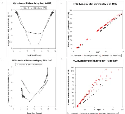
Figure 1 shows examples of the daily variation in NO2 and of the Langley plots pro-duced for the analysis. Multiplying the AMFs by the NO2 chemical ratios from the box model moves both the morning and evening values much closer to a single line, although this line curves down at large values of AMF when using SZAs at the

spec-5

trometer. Using the mean SZAs for the air mass makes the line straighter and the errors smaller.

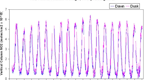
The NO2 vertical columns at twilight produced by the analysis are shown in Fig. 2. The difference between dawn and dusk is greatest during autumn and spring due to the large amounts of N₂O₅at these times, and more variation in the NO₂vertical columns

10

is seen in spring when the site, near the edge of the polar vortex, alternately observes air from inside and outside the vortex. The midsummer and midwinter values vary from year to year, and the lower values of NO2 in December 1991 and all of 1992 are due to the Mt. Pinatubo eruption in June 1991. The eruption greatly increased the amount of aerosols in the stratosphere over the following 18 months, leading to

15

increased hydrolysis of both BrONO2and N2O5to HNO3, which titrates NO2to HNO3. Note that the AMFs in 1991 and 1992 were not changed in this analysis (the error involved is less than 5%, Slusser et al., 1997).

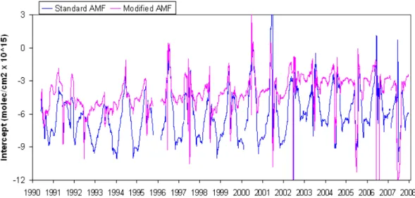
The Langley plot intercepts are shown in Fig. 3. The intercepts have an annual cycle because the wavelength shift varies over the course of the year due to thermal

ex-20

pansion and contraction within the spectrometer. The modified AMFs produce smaller intercepts, particularly in summer, and are closer to the actual slant amount of NO2 in the reference spectrum (3.5×1015molec/cm2). The annual cycle is smaller since the artefacts are smaller and more constant with modified AMFs.

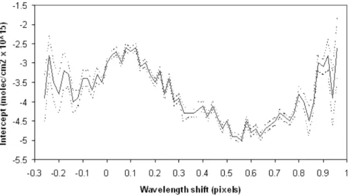
The modified Langley plot intercepts are plotted against the wavelength shift in Fig. 4.

25

(10)

ACPD

9, 837–863, 2009

Title Page

Tables Figures

◭ ◮

Back Close

Full Screen / Esc

Interactive Discussion related to the spectral analysis program searching for minimum residuals, always from

negative to positive wavelength shift. To find the most probable relationship the plot was folded about 0.1 and 0.6 so that all the intercepts lay in the range 0.1 to 0.6, and a best-fit straight line with error was calculated by least-squares fitting.

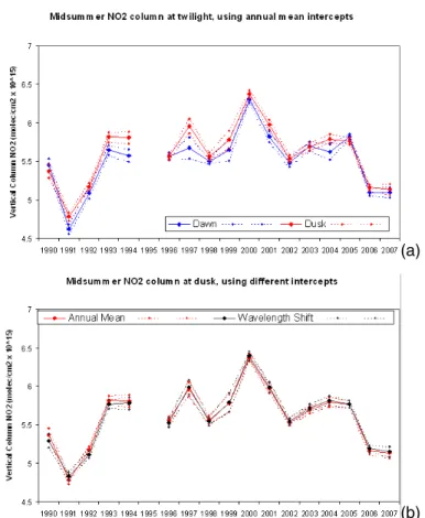
We now look in detail at the analysed NO₂ vertical columns in midsummer, to

con-5

sider any trends in NOy. The midsummer values are the most useful for this because the NO2 columns are largest here, and the N2O5 columns smallest so there is little sensitivity in the NO_y/NO₂ ratio to the amount of aerosols. Figure 5 shows the mid-summer NO2vertical columns, using annual weighted mean intercepts of Fig. 3, and daily intercepts estimated from the wavelength shift in Fig. 4. Considerable

year-to-10

year variation is seen and the values from 1991 and 1992 are low following the Mt. Pinatubo eruption. The pattern of trend and variability is almost identical using the two methods of analysis, with all differences smaller than the errors.

To check that these year-to-year variations are not due to di_fferences in the mean SZA of the measurements, thereby causing a different part of the daily variation to be

15

observed, the midsummer columns were interpolated to 89◦ using the daily variation from the box model. The interpolated columns (not shown) coincide very well, the mean difference is only −0.01×1015molec/cm2, where the dusk and dawn columns have a mean difference of 0.09×1015molec/cm2. This coincidence gives support to the accuracy of the box model simulations. Much the same pattern of trend and variability

20

to that in Fig. 5 is seen, with a broad maximum near 2000. This pattern could be construed as an upwards trend in the NO2 vertical columns between 1990 and 2000 (excluding 1991 and 1992), and a downwards trend after 2000, in which case the gradients of the best-fit lines are given in Table 1. Using wavelength shift intercepts rather than annual mean intercepts again produces a very similar pattern and any

25

differences in the possible trends (Table 1) are not significant.

(11)

sensitiv-ACPD

9, 837–863, 2009

Title Page

Tables Figures

◭ ◮

Back Close

Full Screen / Esc

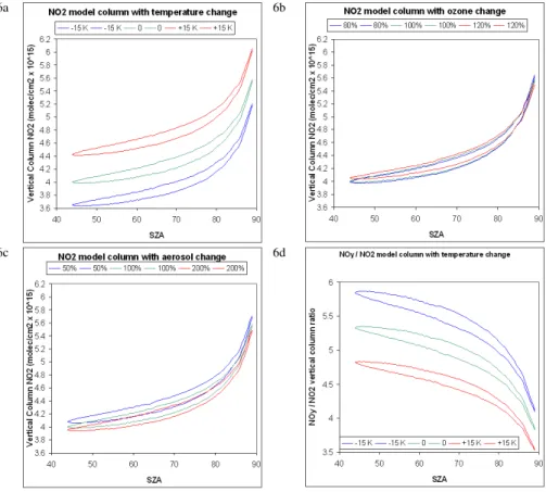
Interactive Discussion ity of the midsummer NO₂vertical column and NO_y/NO₂ratio to these three factors.

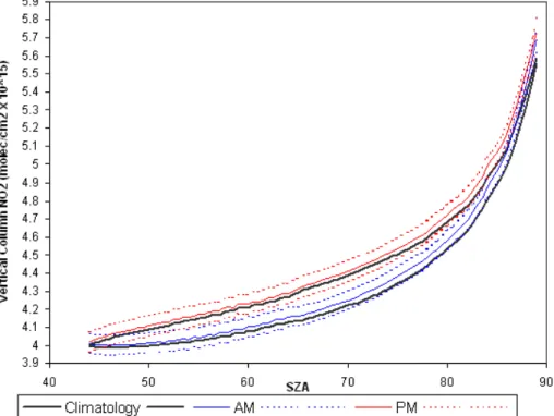
Figure 6a shows the sensitivity of the model NO2vertical column to temperature. In-creasing stratospheric temperature increases NO2while reducing the diurnal variation. These represent large changes in temperature so the sensitivity to realistic changes is modest.

5

Figure 6b shows the sensitivity to ozone. Changing the ozone column will change the amount of UV light reaching different levels of the atmosphere and will also affect the gas phase chemistry. Increasing the ozone reduces the NO2at the same altitude, due to the interaction quantified in Eq. (2) (Roscoe et al., 2001), but has little effect on the overall NO₂column because of the compensating effect of reducing sunlight below,

10

thereby increasing NO₂below.

[NO]

[NO₂]=K₍_J_NO

2)exp(1200/T) .

[O₃] (2)

Figure 6c shows the sensitivity to aerosols, which is set in the box model by changing H2SO4. Increasing the aerosols slightly reduces the NO2 column as more HNO3 is produced, but the effect is small in midsummer. Figure 6d shows the sensitivity of the

15

NO_y/NO₂ratio to temperature, and the ratio is seen to fall with increasing temperature. Using the temperature, ozone and aerosols in the climatology the box model gives a NOy/NO2ratio of 3.8 at 89◦SZA in midsummer.

The partitioning of nitrogen species in the box model at midsummer is most sensitive to temperature with some sensitivity to ozone. Hence to better estimate trends in

20

NO2 and NOy, actual rather than climatological temperature and ozone profiles are needed for each year at midsummer. ECMWF analyses provided temperature and ozone profiles over Faraday and Rothera. The box model was run with these profiles, and the radiative transfer model run with the resulting NO2 and ozone profiles. The box model results for midsummer using the observed and climatological profiles are

25

(12)

ACPD

9, 837–863, 2009

Title Page

Tables Figures

◭ ◮

Back Close

Full Screen / Esc

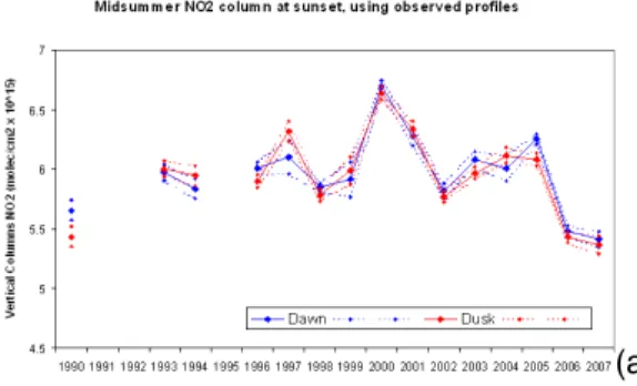
Interactive Discussion Figure 8 shows the midsummer dawn and dusk columns interpolated to 89◦_{, using}

the observed profiles and the climatology. The interpolated columns coincide well, the mean difference is again only−0.01×1015molec/cm2, and they again have much the same pattern of trend and variability as Fig. 5, with a broad maximum near 2000, and the differences from using the climatology or observed profiles are minimal. Again,

5

the pattern could also be construed as an upwards trend before 2000 followed by a downwards trend since, and the gradients of the best-fit lines are given in Table 2.

Figure 9 shows the midsummer NOy vertical columns using the observed profiles and the climatology. The NOy columns are reduced when using the observed profiles, but otherwise the trends and variability are very similar. The gradients of the NO_y

10

best-fit lines are given in Table 2.

Hence using observed profiles of temperature and ozone instead of the climatology makes little difference to the NO₂values and the daily variation from the box model, but makes a significant difference to the NOy values. However the patterns of trend and variability are almost identical irrespective of the method of analysis and irrespective of

15

NO₂or NO_y.

6 Interpretation and conclusion

The atmospheric photochemical box model, the radiative transfer model and the anal-ysis routine form a useful method to analyse NO₂ slant measurements. By creating chemically modified Langley plots, more accurate vertical columns can be calculated,

20

and by using the daily variation of NO2and the ratio of NOy/NO2in the box model the vertical columns of NO_y can be estimated.

The reduction in the NO2 vertical columns in 1991 and 1992, due to increased hy-drolysis of BrONO2 and N2O5 on the aerosols from the Mt. Pinatubo eruption, are clearly seen (Slusser et al., 1997). These years are excluded from further discussion

25

of trends and variability.

(13)

ACPD

9, 837–863, 2009

Title Page

Tables Figures

◭ ◮

Back Close

Full Screen / Esc

Interactive Discussion changes when different intercept values are used, either weighted annual means or

daily values from the wavelength shift. When interpolated to sunset, the dawn and dusk values coincide, giving confidence in the box model simulations. Once again the year-to-year pattern of trend and variability is almost unchanged. It is also almost unchanged when running the models with the observed profiles of temperature and

5

ozone for each year instead of the climatology. All the analyses of NO2 and NOy columns at midsummer have a broad maximum near 2000, with significant interannual variability superimposed and little overall trend between 1990 and 2007 (the overall trend in NOybetween 1990 and 2007 is less than 1%/decade, with a standard deviation of almost 4%/decade). The pattern could aternatively be construed as an increasing

10

trend before 2000 and a decreasing trend since, in which case if we accept the premise that a slower Brewer-Dobson circulation allows more time for a source gas to react to its product, this suggests that the Brewer-Dobson circulation slowed to a minimum around 2000 and has since speeded up.

Earlier studies at 45◦S have identified an increasing trend in NO2 of about 5

15

%/decade between 1980 and 1998 (Liley et al., 2000). If our measurements from 1990 to 2000 are taken as part of the same trend, our result is much larger at about 14%/decade. To discuss the implications in terms of Brewer-Dobson circulation, we must first subtract the trend in tropospheric N2O, the source of stratospheric NOy, which is increasing by about 2.5%/decade (WMO 2007), in which case our trends would be

20

over four times those of (Liley et al., 2000).

An alternative viewpoint is that the changes in NOy mostly consist of inter-annual variability, much of it at sub-decadal scales but some with longer periods. From this viewpoint, the two sets of results could be consistent, because of the large NO2 amounts observed in the early 1980s by Liley et al. (2000), plus our large maximum in

25

NO₂and NO_yin 2000. If so, changes in the Brewer-Dobson circulation are dominated by decadal and sub-decadal variability, and there was a minimum in 2000.

(14)

cor-ACPD

9, 837–863, 2009

Title Page

Tables Figures

◭ ◮

Back Close

Full Screen / Esc

Interactive Discussion related with atmospheric dynamics. Randel et al. (2006) calculated the mean

trop-ical upwelling from the momentum balance in the atmosphere, finding that this de-creased during the 1990s but has inde-creased since 2000, and that both temperature and ozone above the tropical tropopause increased at many longitudes during 1999–2001 which are most probably due to changes in the mean tropical upwelling. Rosenlof and

5

Reid (2008) found that the 1999–2001 warming of the tropical lower stratosphere was very pronounced and that this was strongly correlated with the QBO westerly phase.

Garcia-Herrera et al. (2006) found that the results from general circulation models implied that the El Nino Southern Oscillation (ENSO) signal propagates into the middle atmosphere by means of planetary scale Rossby waves, so that vertical wave

prop-10

agation is enhanced during El Nino events but reduced during La Nina. Zeng and Pyle (2005) found that stratosphere/troposphere exchange increases during El Nino events, but decreases during La Nina. This suggests that the speed of the Brewer-Dobson circulation may depend on ENSO, with a faster circulation during El Nino years (probably resulting in less NOy) and a slower circulation during La Nina years (probably

15

resulting in more NOy). Liley et al. (2000) found an apparent correlation between the NO₂ columns measured at 45◦_{S and ENSO with a time lag of 13 months. Hence the} large peak in NOy in 2000 and the smaller peak in 1997 in this study are consistent with the La Nina events in 1998–2000 and 1996.

Quantitative interpretation of our NO₂ and NO_y trends in terms of changes to the

20

Brewer-Dobson circulation will be presented in future work.

Acknowledgements. Funding was provided by the EU as part of the GEOMON project

(con-tract number 036677). ECMWF operational analyses data and ERA 40 reanalysis data were obtained from the British Atmospheric Data Centre. We thank the WinDOAS authors Michel van Roozendael and Caroline Fayt of IASB, Belgium, and Martyn P. Chipperfield and 25

(15)

ACPD

9, 837–863, 2009

Title Page

Tables Figures

◭ ◮

Back Close

Full Screen / Esc

References

Brewer, A. W.: Evidence for a world circulation provided by the measurements of helium and water vapour distribution in the stratosphere, Q. J. Roy Meteor. Soc., 75, 351–363, 1949. Chipperfield, M. P.: Multiannual simulations with a three-dimensional chemical transport model,

J. Geophys. Res., 104, D1, 1781–1805, 1999. 5

Denis, L., Roscoe, H. K., Chipperfield, M. P., Van Roozendael, M., and Goutail, F.: A new software suite for NO₂vertical profile retrieval from ground-based zenith-sky spectrometers, J. Quant. Spectrosc. Ra., 92, 321–333, 2005.

Dobson, G. M. B.: Origin and distribution of polyatomic molecules in the atmosphere, Proc. R. Soc. Lon. Ser.-A, 236, 187–193, 1956.

10

Garcia-Herrera, R., Calvo, N., Garcia, R. R., and Giorgetta, M. A.: Propagation of ENSO tem-perature signals into the middle atmosphere: A comparison of two general circulation models and ERA-40 reanalysis data, J. Geophys. Res., 111, D06101, doi:10.1029/2005JD006061, 2006.

Lee, A. M., Roscoe, H. K., Oldham, D. J., Squires, J. A. C., Sarkissian, A., Pommereau, J.-P., 15

and Gardiner, B. G.: Improvements to the accuracy of measurements of NO₂by zenith-sky visible spectrometers, J. Quant. Spectrosc. Ra., 52, 5, 649–657, 1994.

Liley, J. B., Johnston, P. V., McKenzie, R. L., Thomas, A. J., and Boyd, I. S.: Stratospheric NO₂variations from a long time series at Lauder, New Zealand, J. Geophys. Res., 105, D9, 11633–11640, 2000.

20

Pommereau, J.-P. and Goutail, F.: O₃and NO₂ ground-based measurements by visible spec-trometry during Arctic winter and spring 1988, Geophys. Res. Lett., 15, 8, 891–894, 1988a. Pommereau, J.-P. and Goutail, F.: Stratospheric O₃and NO₂observations at the southern polar

circle in summer and fall 1988, Geophys. Res. Lett., 15, 8, 895–897, 1988b.

Randel, W. J., Wu, F., Vomel, H., Nedoluha, G. E., and Forster, P.: Deceases in stratospheric 25

water vapor after 2001: Links to changes in the tropical tropopause and the Brewer-Dobson circulation, J. Geophys. Res., 111, D12312, doi:10.1029/2005JD006744, 2006.

Roscoe, H. K., Drummond, J. R., and Jarnot, R. F.: Infrared measurements of stratospheric composition. III, The daytime changes of NO and NO₂, Proc. R. Soc. Lon. Ser.-A, 375, 507– 528, 1981.

30

(16)

ACPD

9, 837–863, 2009

Title Page

Tables Figures

◭ ◮

Back Close

Full Screen / Esc

complete chemical model, J. Quant. Spectrosc. Ra., 68, 337–349, 2001.

Roscoe, H. K.: A review of stratospheric H₂O and NO₂, Adv. Space Res., 34, 1747–1754, 2004.

Rosenlof, K. H. and Reid, G. C.: Trends in the temperature and water vapor content of the tropical lower stratosphere: Sea surface connection, J. Geophys. Res., 113, D06107, 5

doi:10.1029/2007JD009109, 2008.

Sarkissian, A., Roscoe, H. K., and Fish, D. J.: Ozone measurements by zenith-sky spectrom-eters: an evaluation of errors in air-mass factors calculated by radiative transfer models, J. Quant. Spectrosc. Ra., 54, 3, 471–480, 1995.

Slusser, J. R., Fish, D. J., Strong, E. K., Jones, R. L., Roscoe, H. K., and Sarkissian, A.: Five 10

years of NO₂vertical column measurements at Faraday (65◦S): Evidence for the hydrolysis of BrONO₂on Pinatubo aerosols, J. Geophys. Res., 102, D11, 12987–12993, 1997.

Solomon, S., Schmeltekopf, A. L., and Sanders, R. W.: On the interpretation of zenith-sky absorption measurements, J. Geophys. Res., 92, D7, 8311–8319, 1987.

WMO (World Meteorological Organisation), Scientific Assessment of Ozone Depletion: 2006, 15

Global Ozone Research and Monitoring Project – Report No. 50, Geneva, 2007.

(17)

ACPD

9, 837–863, 2009

Title Page

Tables Figures

◭ ◮

Back Close

Full Screen / Esc

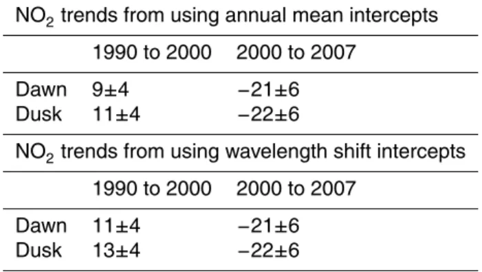
Interactive Discussion Table 1. Trends in the NO₂ vertical column (%/decade) at midsummer sunset between 1990

and 2000 (excluding 1991 and 1992) and between 2000 and 2007, relative to values in 2000. The mean columns at dawn and dusk, calculated using either annual mean intercepts or wave-length shift intercepts, are interpolated to 89◦_{. These trend fits are important for comparison}

with earlier work on trends in NO₂.

NO₂trends from using annual mean intercepts 1990 to 2000 2000 to 2007

Dawn 9±4 −21±6 Dusk 11_±4 ₋22_±6

NO₂trends from using wavelength shift intercepts 1990 to 2000 2000 to 2007

(18)

ACPD

9, 837–863, 2009

Title Page

Tables Figures

◭ ◮

Back Close

Full Screen / Esc

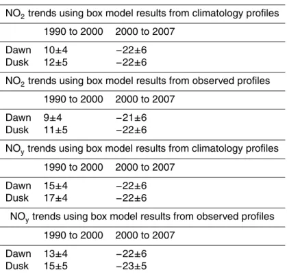
Interactive Discussion Table 2. The trends in the NO₂ and NO_y vertical columns (%/decade) at midsummer sunset

between 1990 and 2000 (excluding 1991 and 1992) and between 2000 and 2007, relative to values in 2000. The mean NO₂columns at dawn and dusk, using either climatology or observed profiles, are interpolated to 89◦_{, then the NO}

ycolumns are calculated from the NOy/NO2ratio

for each year.

NO₂trends using box model results from climatology profiles 1990 to 2000 2000 to 2007

Dawn 10±4 −22±6 Dusk 12±5 −22±6

NO₂trends using box model results from observed profiles 1990 to 2000 2000 to 2007

Dawn 9±4 −21±6 Dusk 11±5 −22±6

NO_ytrends using box model results from climatology profiles 1990 to 2000 2000 to 2007

Dawn 15_±4 ₋22_±6 Dusk 17_±4 ₋22_±6

NO_ytrends using box model results from observed profiles 1990 to 2000 2000 to 2007

(19)

ACPD

9, 837–863, 2009

Title Page

Tables Figures

◭ ◮

Back Close

Full Screen / Esc

Interactive Discussion 1a 1b

1c 1d

(20)

ACPD

9, 837–863, 2009

Title Page

Tables Figures

◭ ◮

Back Close

Full Screen / Esc

Interactive Discussion Fig. 2. The NO₂ vertical columns produced by the analysis at dawn and dusk twilight (87◦ to

92◦_{SZA) with an 11 day running weighted mean, calculated using annual mean intercepts. The}

annual cycle of NO₂with midwinter minima and midsummer maxima is clearly seen, and there is more NO₂at dusk than at dawn. The spectrometer was moved from Faraday (65.25◦_{S) to}

(21)

ACPD

9, 837–863, 2009

Title Page

Tables Figures

◭ ◮

Back Close

Full Screen / Esc

Interactive Discussion Fig. 3. The Langley plot intercepts produced by the analysis using unmodified and modified

(22)

ACPD

9, 837–863, 2009

Title Page

Tables Figures

◭ ◮

Back Close

Full Screen / Esc

Interactive Discussion Fig. 4.The modified Langley plot intercepts versus the wavelength shift after binning, the solid

(23)

ACPD

9, 837–863, 2009

Title Page

Tables Figures

◭ ◮

Back Close

Full Screen / Esc

(a)

(b)

Fig. 5. The midsummer NO₂ vertical columns at twilight (87◦ _{to 92}◦ _{SZA) for each year,}

weighted mean and standard deviation for the days 16 to 26 December. (a)Dawn and dusk columns calculated using annual weighted mean modified Langley plot intercepts, and (b)

(24)

ACPD

9, 837–863, 2009

Title Page

Tables Figures

◭ ◮

Back Close

Full Screen / Esc

6a 6b

6c 6d

Fig. 6. The sensitivity of the box model NO₂ vertical column over Rothera in midsummer to temperature, ozone and aerosols, and the sensitivity of the NO_y/NO₂ ratio to temperature. Each shows the results from 3 simulations, with the unchanged climatology, and with the input values increased and reduced. (a)Stratospheric temperature increased and reduced by 15 K.

(25)