On the Adaptive Partition Approach to the Detection of
Multiple Change-Points
Yinglei Lai*
Department of Statistics and Biostatistics Center, The George Washington University, Washington, D.C., United States of America
Abstract
With an adaptive partition procedure, we can partition a ‘‘time course’’ into consecutive non-overlapped intervals such that the population means/proportions of the observations in two adjacent intervals are significantly different at a given level aC. However, the widely used recursive combination or partition procedures do not guarantee a global optimization. We propose a modified dynamic programming algorithm to achieve a global optimization. Our method can provide consistent estimation results. In a comprehensive simulation study, our method shows an improved performance when it is compared to the recursive combination/partition procedures. In practice,aCcan be determined based on a cross-validation procedure. As an application, we consider the well-known Pima Indian Diabetes data. We explore the relationship among the diabetes risk and several important variables including the plasma glucose concentration, body mass index and age.
Citation:Lai Y (2011) On the Adaptive Partition Approach to the Detection of Multiple Change-Points. PLoS ONE 6(5): e19754. doi:10.1371/journal.pone.0019754
Editor:Mike B. Gravenor, University of Swansea, United Kingdom
ReceivedDecember 10, 2010;AcceptedApril 15, 2011;PublishedMay 24, 2011
Copyright:ß2011 Yinglei Lai. This is an open-access article distributed under the terms of the Creative Commons Attribution License, which permits unrestricted use, distribution, and reproduction in any medium, provided the original author and source are credited.
Funding:This work was supported by the National Institutes of Health grants R21DK075004, R01GM092963 and Samuel W. Greenhouse Biostatistics Research Enhancement Award (GW Biostatistics Center). The funders had no role in study design, data collection and analysis, decision to publish, or preparation of the manuscript.
Competing Interests:The authors have declared that no competing interests exist. * E-mail: [email protected]
Introduction
Time-course data analysis can be common in biomedical studies. A ‘‘time course’’ is not necessarily only a certain period of time in the study. More generally, it can be patients’ age records or biomarkers’ chromosomal locations. A general ‘‘time’’ variable can be a predictor with continuous or ordinal values. When we analyze a response variable (binary, continuous, etc.), it is usually necessary to incorporate the information from this predictor. Many well-developed regression models can be used for the analysis of this type of data. In this study, we focus on a nonparametric type of analysis of time-course data: the whole time course is partitioned into consecutive non-overlapped intervals such that the response observations are similar in the same block but different in adjacent blocks. Then, the partition of time course is actually the detection of change-points. The detection of a single change-point has been well studied in statistical literature [1]. However, for the detection of multiple change-points, since there are many unknown parameters like the number of change-points, the locations of change-points and the population means/ proportions in each block, it still remains a difficult problem [2].
A motivating example for this study is described as follows. The body mass index (BMI) is calculated by dividing the mass (in kilograms) by the square of the height (in meters). The recent WHO classification of BMI gives six categories: underweight (v18.5), normal weight (18.5-24.9), overweight (25.0–29.9), class I obesity (30.0–34.9), class II obesity (35.0–39.9) and class III obesity (w40.0). For the continuous variable BMI, its values are classified into six categories based on five cut-off points. Normal weight is considered as low risk, while the risk of underweight category is elevated, and the risks of overweight, class I, II and III obesity are gradually increased. Therefore, as BMI increases, the risk trend is not simply increasing
nor decreasing, but is a ‘‘U’’ shape. A question motivated from this classification is that, given the data of BMI and health status, can we partition the variable BMI into consecutive non-overlapped intervals (categories) such that the risks are similar within an interval but significantly different between two adjacent intervals?
In this study, our purpose is to partition a ‘‘time course’’ into consecutive non-overlapped intervals such that the population means/proportions of the observations in two adjacent intervals are significantly different at a given levelaC. This type of analysis can provide informative results in practice. For example, medical experts may provide an appropriate consultation based on a patient’s blood pressure level.
The isotonic/monotonic regression (or the order restricted hypothesis testing) is a traditional nonparametric trend analysis of time-course data [3]. Since the maximum likelihood estimation results are increasing/decreasing piecewise constants over the time course, this analysis can also be considered as a special case of change-point problem. Based on the traditional isotonic/mono-tonic regression, the reduced isoisotonic/mono-tonic/monoisotonic/mono-tonic regression has been proposed so that the estimation results can be further simplified [4]. Its additional requirement is that the estimated population means in two adjacent blocks must be significantly different at a given level. However, the existing method is based on a backward elimination procedure and does not guarantee the maximum likelihood estimation results.
piecewise constants. This method has been frequently used for analyzing array-CGH data [6]. The reduced isotonic regression (see above) is an example of recursive combination. These recursive algorithms provide approximated solutions as alterna-tives to the globally optimized solutions since an exhaustive search is usually not feasible. Therefore, global optimizations are not always guaranteed.
The dynamic programming algorithm is a frequently used method for optimizing an objective function with ordered observations [7]. Therefore, it is intuitive to consider this algorithm in the analysis of time-course data. This algorithm has actually been frequently used to implement many statistical and computational methods [8][9][10][11][12][13]. For a feasible implementation of this algorithm, an optimal sub-structure is necessary for the objective function. This is usually the case for the likelihood based estimation in an unrestricted parameter space. However, when there are restrictions for the parameters, certain modifications are necessary for the implementation of the dynamic programming algorithm.
In the following sections, we first present a modified dynamic programming algorithm so that a global optimization can be achieved for our analysis. The algorithm has been originally developed for the normal response variables. But the extension of our method to the binary response variable is straightforward and is also discussed later. We prove that this method can provide consistent estimation results. Then, we suggest a permutation procedure for thep-value calculation and a bootstrap procedure for the construction of time-point-wise confidence intervals. We use simulated data to compare our method to the recursive combina-tion/partition procedures. The well-known Pima Indian Diabetes data set is considered as an application of our method. We explore the relationship among the diabetes risk and several important variables including the plasma glucose concentration (in an oral glucose tolerance test, or OGTT), body mass index (BMI) and age.
Methods
A modified dynamic programming
At the beginning, we introduce some necessary mathematical notations. Consider a simple data set with two variables:
X~fx1vx2v. . .vxmg represents m distinct ordered indices
(referred to as ‘‘time points’’ thereafter), and Y~fykl:
k~1,2,. . .,m;l~1,2,. . .,nkg represents the observations with yklbeing thel-th observation at thek-th time point. Letfmkgbe
the corresponding population mean ofY at thek-th time point.
We assume thatykl~mkzekl, wherefeklgare independently and identically distributed (i.i.d.) with the normal distributionN(0,s2).
Furthermore, we assume that the set fmkg has a structure
fm1~. . .~mm1=mm1z1~. . .~mm1zm2=. . .=mm1zm2z...zmg{1z1 ~mm1zm2z...zmg{1zmgg with m1zm2z. . .zmg~m. fmkg, s
2
and the setfm1,m2,. . .,mggare all unknown (includingg) and to be estimated.
The traditional change-point problem assumes thatg~2. When
gw2, it is a multiple change-point problem. If there is no strong evidence of change points, we may consider the null hypothesis of no change-point (g~1)H0:fmkgare the same. For the traditional analysis of variance (ANOVA), we consider an alternative hypothesisHa: fmkgcan be different. Then, even when the null
hypothesisH0can be significantly rejected, there may be many
adjacentfmkgestimated with similar values. Therefore, we intend
to group similar and adjacent fmkg into a block. If this is
achievable, then we can have a detection of multiple change-points. Therefore, we specify the following restricted parameter space for the alternative hypothesis:
V1:fmkgcan be different; if we claim anymk=mkz1, then they are significantly different at levelaC by a two-tailed (or upper-tailed/lower-tailed) test with the two-sample data partitioned to includemkandmkz1in each sample.
Remark 1. The comparison based on adjacent time points
has no effect andV1is reduced toHawhenaC~1. Clearly,V1is
reduced toH0whenaC~0. Furthermore, when an upper-tailed/
lower-tailed test is specified, the analysis is the reduced isotonic/ monotonic regression [4]. Particularly, the analysis is the
traditional isotonic/monotonic regression [3] when aC~0:5
(when a one-sidedt-test is used for comparing two sample groups).
The goal of this study is to partitionX into consecutive
non-overlapped intervals such that the population means of the observations in two adjacent intervals are significantly different at a given levelaC. This type of analysis cannot be achieved by the computational methods for the order restricted hypothesis testing (or the isotonic regression) due to the existence of significance parameter. One may consider the well-known dynamic program-ming (DP) algorithm [7] since the observations are collected at consecutive time points. This is again not feasible: an optimized partition for a subset of time points may be excluded for a larger
set of time points due to the significance requirement in V1.
However, we realize that the traditional DP algorithm can be
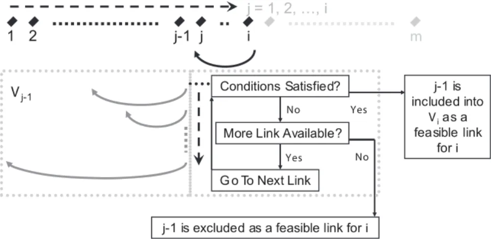
Figure 1. An illustrative flow chat for the modified dynamic programming algorithm.
modified to achieve our goal by adding an additional screening step at each time point.
Algorithm. Due to its satisfactory statistical properties, the
likelihood ratio based test (LRT) has been widely used. To conduct a LRT, we need to estimate the parameters under different hypotheses. When normal population distributions (with a
common variance) are assumed for Y, the maximum likelihood
estimation is equivalent to the estimation by minimizing the sum of squared errors (SSE). When a block of time points fxj,xjz1,. . .,xig are given, the associated SSE is simply
s(j,jz1,. . .,i)~Pi
k~j
Pnk
l~1(ykl{yyj,...,i)2, where yyj,...,i is the
sample mean of the observations in the time block
fxj,xjz1,. . .,xig. Notice that the SSE of several blocks is simply the sum of SSEs of individual blocks. Then, under the alternative hypothesis, we propose the following algorithm that is modified based on the well-known DP algorithm. For simplicity, we refer to the term ‘‘triplet’’ as a vector containing (link, index, score) that are described in the algorithm. (For each triplet, ‘‘link’’ is defined as the time point right before the block under current consideration; ‘‘index’’ is defined as the index in the triplet set linked from the time point under current
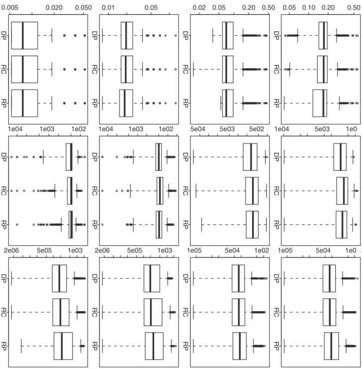
Figure 2. Simulation based comparison of the overall mean squared errors.All y-axes represent the overall mean squared error. DP represents our dynamic programming algorithm; RC and RP represent the recursive combination and recursive partition algorithms, respectively. The boxplots in each row (1–4) are generated from the analysis results based on the corresponding simulation scenario (1–4). The boxplots in each column (1–3) are generated from the analysis results based on differentnk(1, 10 and 100).
consideration; ‘‘score’’ is defined as the objective function value under current consideration.)
link/0; index/0; score/s(1)
CreateV1as a vector set with only one element with the above
triplet
fori~2tomdof
link/0; index/0; score/s(1,2,. . .,i)
CreateVias a vector set with only one element with the
above triplet
forj~2toidof
Go throughVj{1as ordered until a feasible index can
be foundf
link/j{1
index/current position inVj{1
score/(current score inVj{1)+s(j,jz1,. . .,i)
Include the above triplet as a new element in Vi
g g
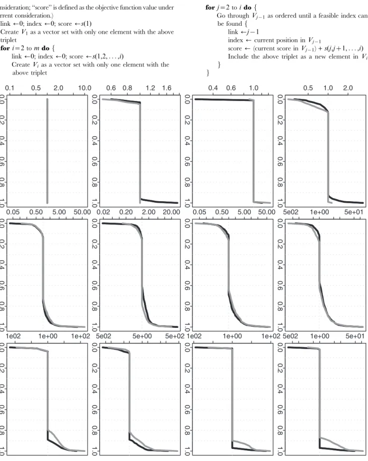
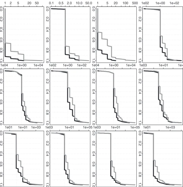
Figure 3. Simulation based comparison of the overall mean squared errors.All y-axes represent the quantile of relative ratio of overall MSEs given by each of the two approximation methods vs. our proposed method. All x-axes represent the values used to calculate the empirical quantiles. The black curves represent RC vs. DP and the gray curves represent RP vs. DP. (DP represents our dynamic programming algorithm; RC and RP represent the recursive combination and recursive partition algorithms, respectively.) The plots in each row (1–4) are generated from the analysis results based on the corresponding simulation scenario (1–4). The plots in each column (1–3) are generated from the analysis results based on differentnk(1, 10 and 100).
SortViaccording to the increasing order of SSE scores g
Remark 2. It is important that the maximum likelihood
estimation is equivalent to the estimation by minimizing the sum of squared errors (SSE) when normal population distributions (with a
common variance) are assumed for Y. Notice that a normal
distribution is assumed for each time point. The population means can be different at different time points but the population variances are common for all the time points. Due to the optimal
substructure requirement for the dynamic programming
algorithm, we can only estimate the parameters specific to the existing partitioned blocks. As shown in the above algorithm, the estimation of variance can be achieved after the estimation of population means. (The algorithm will not work if the common population variance has to be estimated within the algorithm.)
Remark 3. The definition for a feasible index in Vj{1 is a
time point h such that two population means in the blocks
fh,hz1,. . .,j{1gandfj,jz1,. . .,igare significantly different at levelaC(as specified in the restricted parameter spaceV1). A flow chat is given in Figure 1 to illustrate this algorithm. The setVi
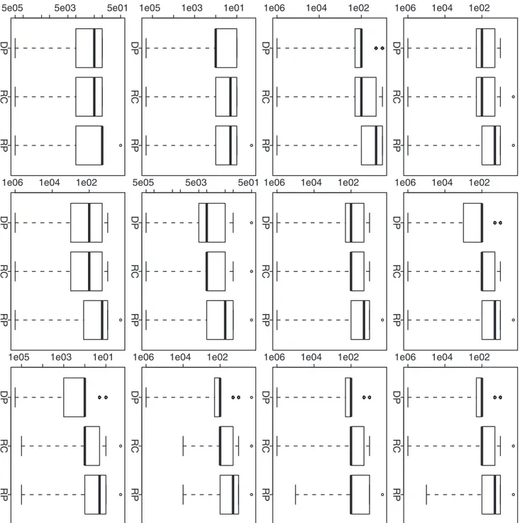
Figure 4. Simulation based comparison of the selectedaC.All y-axes represent the selectedaC. DP represents our dynamic programming
algorithm; RC and RP represent the recursive combination and recursive partition algorithms, respectively. The boxplots in each row (1–4) are generated from the analysis results based on the corresponding simulation scenario (1–4). The boxplots in each column (1–3) are generated from the analysis results based on differentnk(1, 10 and 100).
contains an optimized link index among the feasible ones for each of its previous time pointj{1,j~1,2,. . .,i(if there is no feasible
link index for a previous time point j{1, then j{1 will be
excluded fromVi). Since the required condition for the restricted
population means are imposed on adjacent blocks, the setVialso
contains all the necessary link point for the future time points when
the time point i is screened as a link point. (Then, it is not
necessary to check other time pointsjvinot included inVi.) This can be confirmed as follows: if any future time point uses the time
pointias a link point, then any sub-partitions stopped at the time
point i must meet the required conditions for the restricted
population means; furthermore, an optimized one will be chosen from the feasible ones for each time point before the time pointi; therefore, these sub-partitions belong toVi.
Theorem 1. With the mathematical assumptions described at
the beginning, the proposed modified dynamic programming algorithm solves the maximum likelihood estimation of restricted population means.
Figure 5. Simulation based comparison of the selectedaC.All y-axes represent the quantile of relative ratio ofaC’s from each of the two
approximation methods vs. our proposed method. All x-axes represent the values used to calculate the empirical quantiles. The black curves represent RC vs. DP and the gray curves represent RP vs. DP. (DP represents our dynamic programming algorithm; RC and RP represent the recursive combination and recursive partition algorithms, respectively.) The plots in each row (1–4) are generated from the analysis results based on the corresponding simulation scenario (1–4). The plots in each column (1–3) are generated from the analysis results based on differentnk(1, 10 and 100).
Proof:With the above discussion, it is not difficult to give a proof. It is obvious to prove this claim at the time points 1 and 2 since the algorithm just enumerates all possible partitions and selects the optimized one. Assume that the claim holds at the time point k. For the time point kz1, the algorithm screens all the previous time points and selects the optimized and feasible solution (when it exists) for each of them. Finally, all these locally optimized solutions are sorted so that a global optimized solution can be found. Therefore, the claim also holds at the time pointkz1. This concludes the proof that the claim holds for all the time points.
Remark 4. To test whether mk=mkz1 (or mkvmkz1 or
mkwmkz1) is significant at level aC, we consider the well-known two-sample Student’st-test. The statistical significance (p-value) of a test value can be evaluated based on the theoreticalt-distribution or through the permutation procedure [14]. Considering the likely small sample size on each time point and the computing burden
involved in this analysis, the theoretical p-value may be a more
preferred choice when the observations are approximately normally distributed. (The required sample size for calculating a
p-value is no less than two for each sample; otherwise, one will be considered as the reportedp-value.)
Estimators. When we finish screening the last time points,
the overall optimized partition can be obtained in a backward manner:
i/m; h/1
Create the setCwith an elementm
whilehw0dof
j/i; i/Vj:zlink½h; h/Vj:index½h
Includeias a new element in the setC
g
The estimated meansfmm^kgin the restricted parameter spaceV1 are simply the sample means for the partitioned blocks. Withf^mmkg
calculated, we can estimate the variance by ss^2~Pmk~1
Pnk
l~1ðykl{mm^kÞ2
. Pm
k~1nk{1:
Compared to the traditional dynamic programming algorithm,
which requires O(m2) computing time, our modified algorithm
requires at leastO(m2)but at mostO(m3)computing time. The additional computing time is necessary so that the optimization can be achieved in the restricted parameter spaceV1.
Consistency of Estimation
The following theorem shows that our proposed algorithm can provide consistent estimates forfmk:k~1,2,. . .,mgands2. The mathematical proof is given in File S1.
Theorem 2. Let n~Pmk~1nk. Assume that 0va
vnk=nvbv1 and aCw0. Then, for any time point xk, we
have limnk??mm^k?mkin probability:Furthermore, we also have limn??^ss2?s2in probability:
Here, we briefly provide an outline of proof for the readers who wish to skip the mathematical derivation. When the sample size at each time point becomes larger and larger, eventually the true structure f½x1,. . .,xm1, ½xm1z1,. . .,xm1zm2, . . ., ½xm1zm2z...zmg{1z1, . . .,xm1zm2z...zmgg will be a feasible partition of time points (since the power of the two-sample tests for these adjacent partitions will go to 100%). Its corresponding estimates are actually the sample means and they are consistent estimators. Furthermore, the estimated variance, which is closely related to the SSE, will be eventually optimal when the sample size becomes larger and larger. However, our algorithm
guarantees a minimized SSE. Then, the estimated population means provided by our algorithm will be closer and closer to the underlying sample means. Therefore, our algorithm can provide consistent estimates for the underlying population means. Then, it is straightforward to prove the convergence of the variance estimator.
Remark 5. The estimation bias and variance for isotonic
regression are difficult problems [15][16][17]. These two issues are even more difficult for our adaptive partition approach since a two-sample test is involved in the detection of multiple change-points. (However, the building-in two-sample test can be an appealing feature for practitioners.) Therefore, we use the well-known permutation and bootstrap procedures to obtain the
p-value of test and the confidence limits of estimates. They are
briefly described as below.
F-type test and itsp-value
We use SSE1 to denote the score in the first element ofVm.
This is the optimized SSE associated with the restricted parameter
spaceV1. The SSE associated with the null hypothesis is simply
SSE0~Pmk~1
Pnk
l~1(ykl{yy1,...,m)2. Then, we can define aF-type test:
F~SSE0{SSE1
SSE1
Pm
k~1nk{m
m{1 :
It is straightforward to show thatF is actually a likelihood ratio test. However, it is difficult to derive the null distribution ofFdue to the complexity of our algorithm. Therefore, we propose the following permutation procedure for generating an empirical null distribution.
1. Generate Y~fykl:k~1,2,. . .,m;l~1,2,. . .,nkgas a
ran-dom sample (without replacement) fromY~fyklg;
2. Run the modified DP algorithm withXandYas input and
calculate the associatedF-type testF;
3. Repeat steps 1&2Btimes to obtain a collection of permutedF
-scores fFg, which can be considered as an empirical null
distribution.
The procedure essentially breaks the association betweenYand
X. It is also equivalent to permute the expanded time point setXX~
(see below). In this way, the null hypothesis can be simulated with
the observed data and the null distribution of F can be
approximated after many permutations [18]. Then, the p-value
of an observedF-score can be computed as: (number ofF§F)/
B. For a conservative strategy, we can include the observedFinto
the set of permuted F-scores (since the original order is also a
permutation). We can use this strategy to avoid zerop-values.
Time-point-wise confidence intervals
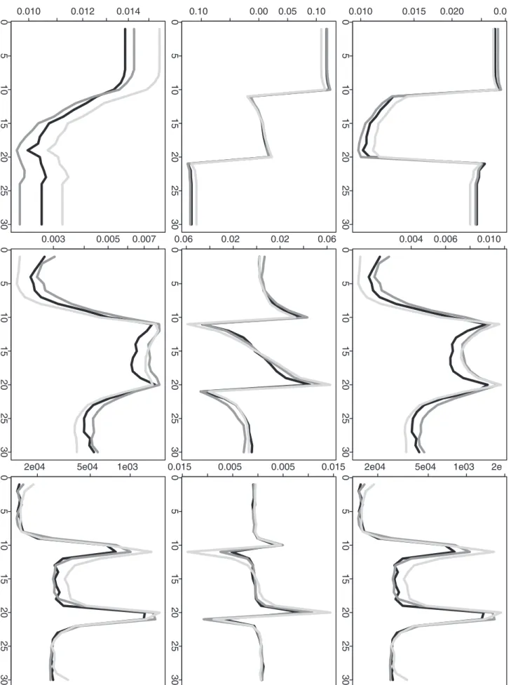
Our algorithm provides an estimate of population mean at each time point. It is difficult to derive the theoretical formula for constructing a confidence interval. Instead, we can consider a bootstrap procedure. At the beginning, we need to expand the variable X~fx1vx2v. . .vxmg to XX~~f~xxkl:k~1,2,. . .,m; l~1,2,. . .,nkg, where xx~kl~xk for l~1,2,. . .,nk. Then, we denote(XX~,Y)~f(xx~kl,ykl):k~1,2,. . .,m;l~1,2,. . .,nkg. Figure 6. Simulation based comparison of time-point-wise MSE, bias and variance.The y-axes represent the time-point-wise MSE (upper row), bias (middle row) or variance (lower row). The x-axes represent the time point. The plots are generated from the analysis results based on the simulation scenario 1. The plots in each column (1–3) are generated from the analysis results based on differentnk(1, 10 and 100).
1. Generate(XX~,Y)~f(~xx
kl,ykl):k~1,2,. . .,m;l~1,2,. . .,nkg, where(~xx::,y::)is re-sampled based on(XX~,Y)with replacement;
2. Run the modified DP algorithm withXX~andYand estimate
the time-point-wise population means; if any time points inX
is not re-sampled in XX~, then assign missing values as the estimates for those time points;
3. Repeat steps 1&2Btimes to obtain a collection of resample estimates of time-point-wise population meansf^mmkg.
The procedure applies the ‘‘plug-in principle’’ so that a resample distribution can be generated for each time point [19]. A pair of empirical percentiles (e.g. 2.5% and 97.5%) can be used to constructed a confidence interval for each time point after excluding the missing values.
Extension to binary response variables
It is straightforward to extend our method for the binary response variables. This can be simply achieved by changing the objective function (SSE in our current algorithm) to the corresponding (negative) log-likelihood function for the binary response variable, and also changing the two-samplet-test in our current algorithm to the corresponding two-sample comparison test for the binary response variable. Due to the computing
burden, we would suggest to use the two-sample z-test for
proportions when there is a satisfactory sample size or the Fisher’s exact test when the sample size is small (e.g. less than six in each cell of the 262 contingency table).
Choice of aC
An appropriate choice ofaC is important. A small number of
partitioned blocks will be obtained if a small value is set foraC, and
vice versa. For examples, no partition will be obtained ifaC~0
and each time point will be a partition ifaC~1. Therefore, like the smoother span parameter for the local regression [20],aCcan also be considered as a smoothing parameter. In practice, we suggest to
use the cross-validation procedure [21] to select aC. Among a
given finite set of values likef0:5,0:1,. . .,0:000005,0:000001g, we can choose the one that minimizes the prediction error.
Approximation algorithms: recursive combination and recursive partition
To illustrate the advantage of global optimization in the likelihood estimation of restricted population means, we also consider and implement two widely used approximation algo-rithms: recursive combination and recursive partition. These algorithms provide approximated (sometimes exact) solutions to the optimal solution in the restricted parameter space defined based on the givenaC. Based on the following description of these two algorithm, it is clear their required computing time is at most
O(m2).
For the recursive combination algorithm, it begins with no partition and each time point is a block. In each loop, it conducts a two-sample test for each pair of adjacent blocks and
find these pairs with p-value higher than aC; among the
combinations based on these selected pairs of adjacent blocks, the one that results the largest overall likelihood (based on all the data) is chosen and the next loop is started when it is still possible to combine the existing blocks; otherwise, the algorithm
stops and returns the partitioned blocks. [Notice that this algorithm is slightly different from the one proposed by [4], in which the pair of blocks is chosen completely based on the two-sample test. In our simulation studies, we have observed that the likelihood based criterion can result in a better performance (results not shown).]
For the recursive partition algorithm, it begins with one block with all the time points. In each loop, within each existing partitioned block, it conducts a two-sample test for each possible partition (that generates two smaller blocks) and find these triplets (when the partitions are from the blocks in the middle of time course) or pairs (when the partitions are from the blocks on the boundaries of time course) with test
p-values lower than aC; among the partitions based on these
selected triplets/pairs, the one that results the largest overall likelihood (based on all the data) is chosen and the next loop is started when it is still possible to create new partitions; otherwise, the algorithm stops and returns the partitioned blocks.
Performance evaluation
In a cross-validation (CV) procedure (e.g. leave-one-out or
10-fold CV), the estimated population mean mm^(k{kl) for each
observation ykl can be obtained based on the training data
withoutykl. (If the time pointxkis not included in the training set, then^mm(k{kl)can still be obtained based on the linear interpolation between two nearest time points toxk.) Then, the CV (prediction)
error is calculated as X
k
X
l(ykl{mm^
({kl)
k )
2:
Remark 6. In a simulation study, instead of a CV error, we can
use the overall mean squared error since we know the parameter values. This is a strategy to save a significant amount of computing time. For each round of simulation, the overall mean squared error
is calculated as P
k
P
l(ykl{^mmk)2
Pm
k~1
Pnk l~1
. After B
rounds of simulations and estimations (including the selection of aC), it is also statistically interesting to understand the estimation mean squared error (MSE), bias and variance at each time point. The time-point-wise mean squared error, bias and variance (for the
k-th time point, k~1,2,. . .,m) are calculated as: MSEk~
PB
i~1 mm^ (i)
k{mk
2
B;Biask~PBi~1 mm^ (i)
k{mk
.
B;Variancek~
PB
i~1 mm^ (i)
k{
PB
j~1mm^ (j)
k
. B
2
B. Notice that the denominator for
Variancek is B instead of B{1 such that MSEk~
Bias2
kzVariancek.
Results
Simulation studies
We consider four simple scenarios to simulate time-course data: (1) m1~m2~. . .~m10~0, m11~m12~. . .~m20~0:5, m21~m22 ~. . .~m30~1,ykl*Normal(mk,1); (2)m1~m2~. . .~m10~0:5, m11~m12~. . .~m20~0, m21~m22~. . .~m30~0:5, ykl* Normal(mk,1); (3) m1~m2~. . .~m10~0:15, m11~m12~. . . ~m20~0:3, m21~m22~. . .~m30~0:45, ykl*Bernoulli(mk); (4) m1~m2~. . .~m10~0:3, m11~m12~. . .~m20~0:15, m21~m22 ~. . .~m30~0:3, ykl*Bernoulli(mk). For each scenario, the number of observations isnk~1, 10, or 100 at every time point. For each simulated data set, we consider twelve different values of aC[f0:5,0:1,0:005,. . .,0:000001g. Two-tailed tests are used so Figure 7. Simulation based comparison of time-point-wise MSE, bias and variance.The y-axes represent the time-point-wise MSE (upper row), bias (middle row) or variance (lower row). The x-axes represent the time point. The plots are generated from the analysis results based on the simulation scenario 2. The plots in each column (1–3) are generated from the analysis results based on differentnk(1, 10 and 100).
Figure 8. Simulation based comparison of time-point-wise MSE, bias and variance.The y-axes represent the time-point-wise MSE (upper row), bias (middle row) or variance (lower row). The x-axes represent the time point. The plots are generated from the analysis results based on the simulation scenario 3. The plots in each column (1–3) are generated from the analysis results based on differentnk(1, 10 and 100).
that no monotonic changes are assumed. Since we know the true parameters for simulations, we choose theaCvalue that minimizes the overall mean squared error (MSE). This makes our simulation study computationally feasible since it is difficult to run the cross-validation procedure for many simulation repetitions. Then, for each round of simulation, we obtain the ‘‘optimized’’ overall MSE
and the corresponding aC for each of the three algorithms: the
global optimization algorithm (our dynamic programming algo-rithm) and two approximation algorithms (the recursive combi-nation algorithm and the recursive partition algorithm). After 1000 repetitions, we compare the boxplots of these two results. A lower overall MSE is obviously preferred. But a loweraCvalue can also be preferred since the detected changes will be statistically more significant. (aCcan be considered as a smoothing parameter if we do not have a pre-specified value for it. However, it also defines the significant level for the test between any two adjacent blocks. Then, a smalleraCindicates a more significant testing results and it is more preferred.) Therefore, a lower boxplot means a better performance for both results.
For all the above four scenarios, Figures 2 and 4 shows similar
patterns. When nk is as small as one for each time point, the
approximation algorithms give a better performance in term of overall MSE, but the global optimization algorithm still gives a quite comparable performance (Figure 2); on the choice ofaC, the global optimization algorithm gives a better performance and the approximation algorithms can give a comparable performance
(Figure 4). When nk becomes larger to 10 and then to 100, we
observe a clear performance improvement from the global optimization algorithm: we can achieve a clearly smaller overall
MSE and also much more significantaC(Figures 2 and 4).
To further compare the performance of three different methods, we calculate the relative ratio between two overall MSEs (or the
selected aC’s) given by each of the two approximation methods
(RC or RP) vs. our proposed method (DP). Based onB~1000
simulation repetitions, we can understand the empirical distribu-tions of these ratios. If any ratio distribution is always no less than one, then DP is absolutely a better choice. Furthermore, for a ratio distribution, If the proportion of (ratiow1) is clearly larger than the proportion of (ratiov1), then DP is still a preferred choice in practice. Corresponding to Figure 2, Figure 3 further demonstrates the advantage of DP when the sample size is not relatively small. Even when the sample size is as small as one at each time point, DP still shows a quite comparable performance. For the selected aC, Figure 5 corresponds to Figure 4 and it also further confirms
the advantage of DP. [In each plot, the proportion of (ratiow1) is cumulated from the right end although the proportion of (ratio
v1) is cumulated from the left end.]
In addition to the overall performance based on the overall
MSE and the selected aC, it is also statistically interesting to
understand the estimation mean squared error, bias and variance at each time point. The time-point-wise mean squared error (MSE), bias and variance (for thek-th time point,k~1,2,. . .,m) are shown in Figures 6, 7, 8, 9 for three different methods. For the time-point-wise MSE, even when the sample size is relatively small (one observation at each time point), our proposed method (DP) still shows an overall comparable performance when it is compared to the two approximation methods (RC or RP). As the sample size is increased, its time-point-wise MSEs become overall comparably lower and lower. For the time-point-wise bias, when sample size is relatively small (one at each time point), DP shows an overall worse performance in the simulation scenarios 1 and 3 but it still shows an overall comparable performance in the simulation scenarios 2 and 4. As the sample size is increased, its biases become overall comparably lower and lower (i.e. closer to the zero y-axis value). For the time-point-wise variance, DP always shows an overall comparable performance. (When the sample size is as small as one at each time point, the estimated time-point-wise means are almost all constants from all three different methods in the simulation scenarios 2; then the corresponding time-point-wise variance patterns are relatively flat. For the same sample size, the estimated time-point-wise means are actually all constants from all three different methods in the simulation scenarios 4; then the corresponding time-point-wise variances are actually constant across the whole time period. This also explains the relatively regular patterns of the corresponding time-point-wise MSE and bias.)
Applications
For applications, we consider different univariate analysis scenarios for the well-known Pima Indian diabetes data [22]. The data set contains a binary variable for the indication of diabetes and three continuous variables for the plasma glucose concentration at 2 hours in an oral glucose tolerance test (OGTT), BMI and age (other variables in this data set are not considered in our study). Our proposed method allows us to detect the multiple change-points for diabetes indication vs. OGTT, BMI or age (analysis for a binary response), and also OGTT vs. BMI or age (analysis for a continuous response). To reduce the computation burden, the observed OGTT Figure 9. Simulation based comparison of time-point-wise MSE, bias and variance.The y-axes represent the time-point-wise MSE (upper row), bias (middle row) or variance (lower row). The x-axes represent the time point. The plots are generated from the analysis results based on the simulation scenario 4. The plots in each column (1–3) are generated from the analysis results based on differentnk(1, 10 and 100).
doi:10.1371/journal.pone.0019754.g009
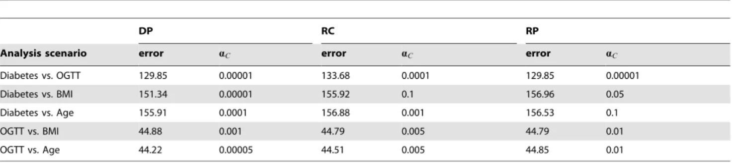
Table 1.Comparison of the leave-one-out cross-validation errors and the selectedaC’s.
DP RC RP
Analysis scenario error aC error aC error aC
Diabetes vs. OGTT 129.85 0.00001 133.68 0.0001 129.85 0.00001
Diabetes vs. BMI 151.34 0.00001 155.92 0.1 156.96 0.05
Diabetes vs. Age 155.91 0.0001 156.88 0.001 156.53 0.1
OGTT vs. BMI 44.88 0.001 44.79 0.005 44.79 0.01
OGTT vs. Age 44.22 0.00005 44.51 0.005 44.85 0.01
values are rounded to the nearest 5 units and the observed BMI values are rounded to the nearest 1 unit when any of these two variables is considered as a ‘‘time’’ variable.aCis chosen from the finite set of values aC[f0:5,0:1,0:05,. . .,0:000001g to minimize the leave-one-out cross-validation (LOO-CV) prediction error. Two-tailed tests are used so that no monotonic changes are assumed. Again, we compare three algorithms: the global optimization algorithm (our dynamic programming algorithm) and two approximation algorithms (the recursive combination algorithm and the recursive partition algorithm).
For each analysis scenario and each algorithm, Table 1 gives
the ‘‘optimized’’ LOO-CV error and the correspondingaC. The
global optimization algorithm always chooses a highly significant
aC while the approximation algorithms sometimes choose a
relatively large value ofaC. In term of prediction error, the global optimization algorithm achieves the best performance in four out of five scenarios. Although the approximation algorithms give the best prediction error for the analysis of OGTT vs. BMI, the global optimization algorithm only gives a slightly worse prediction error.
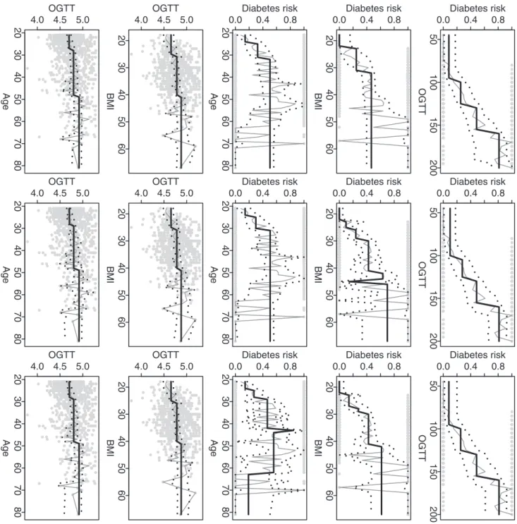
Figure 10 shows the identified change-points for all five analysis scenarios and also all three algorithms. The global optimization algorithm always gives stable change patterns while the approx-imation algorithms sometimes give abrupt drops or jumps. The change patterns fitted by the global optimization algorithm are all increasing and this is practically meaningful. For example, the analysis result for diabetes indication vs. OGTT suggests significant increasing risks of diabetes when OGTT values are
increased to w100, w130 and w160; the analysis result for
diabetes indication vs. BMI suggest significant increasing risks of
diabetes when BMI values are increased to w23 andw32; and
the analysis results for diabetes indication vs. age suggest
significant increasing risks of diabetes when age values arew25
andw32. Since OGTT is an important predictor for diabetes, it is also interesting to understand its changes over different BMI or age intervals. Figure 10 shows increasing patterns for OGTT vs. BMI and OGTT vs. age. The change-points identified by the
global optimization algorithm arew25 andw40 for OGTT vs.
BMI, andw27 andw48 for OGTT vs. age.
Discussion
The advantage of our proposed method is that the maximum likelihood estimation can be achieved during the partition of a time course. Furthermore, the method is simple and the interpretation of estimation results is clear. Based on our knowledge, the modified dynamic programming algorithm proposed in this study is novel. Although the algorithm requires more computing time than does the traditional dynamic programming algorithm, it is still practically feasible with the current computing power for general scientists. We have demonstrated the use of our algorithm for normal and binary response variables. It is also feasible to modify the algorithm for other types of response variables. Furthermore, it is interesting to explore whether there are better approaches to the choice ofaC. These research topics will be pursued in the near future.
One disadvantage of our method, which is actually a common disadvantage for general nonparametric methods, is that a relatively large sample size is required in order to achieve a satisfactory detection power. (This is consistent with the results in Figure 2.) For our method, we would require a relatively long time course, or a relatively large number of observations at each time point. In our simulation and application studies, we choose to analyze the data sets with relatively long time courses since this well illustrates the advantage of our method.
Our method may also be useful for the current wealthy collection of genomics data. For example, we can apply the method to array-based comparative genomics hybridization (aCGH) data and identify chromosomal aberration/alteration regions [6]; we can also apply the method to certain time-course microarray gene expression data and cluster different genes based on their changing pattern across the time course. However, a powerful computer workstation/cluster may be necessary due to the relatively high computing burden from our method.
Supporting Information
File S1
(PDF)
Acknowledgments
I am grateful to Drs. Joseph Gastwirth, John Lachin, Paul Albert, Hosam Mahmoud, Tapan Nayak, and Qing Pan for their helpful comments and suggestions. The R-functions implementing our method and the illustrative examples are available at: http://home.gwu.edu/˜ylai/research/FlexStepReg.
Author Contributions
Conceived and designed the experiments: YL. Performed the experiments: YL. Analyzed the data: YL. Contributed reagents/materials/analysis tools: YL. Wrote the paper: YL.
References
1. Siegmund D, Venkatraman ES (1995) Using the generalized likelihood ratio statistic for sequential detection of a change-point. The Annals of Statistics 23: 255–271. 2. Braun JV, Muller HG (1998) Statistical methods for DNA sequence
segmentation. Statistical Science 13: 142–162.
3. Silvapulle MJ, Sen PK (2004) Constrained statistical inference. Hoboken, New Jersey, USA: John Wiley & Sons, Inc.
4. Schell MJ, Singh B (1997) The reduced monotonic regression model. Journal of the American Statistical Association 92: 128–135.
5. Olshen AB, Venkatraman ES, Lucito R, Wigler M (2004) Circular binary segmentation for the analysis of array-based DNA copy number data. Biostatistics 5: 557–572.
6. Venkatraman ES, Olshen AB (2007) A faster circular binary segmentation algorithm for the analysis of array CGH data. Bioinformatics 23: 657–663. 7. Cormen TH, Leiserson CE, Rivest RL, Stein C (2001) Introduction to
Algorithms, 2nd edition. MIT Press & McGraw-Hill.
8. Autio R, Hautaniemi S, Kauraniemi P, Yli-Harja O, Astola J, et al. (2003) CGH-plotter: MATLAB toolbox for CGH-data analysis. Bioinformatics 19: 1714–1715. 9. Picard F, Robin S, Lavielle M, Vaisse C, Daudin JJ (2005) A statistical approach
for array CGH data analysis. BMC Bioinformatics 6: 27.
10. Price TS, Regan R, Mott R, Hedman A, Honey B, et al. (2005) SW-ARRAY: a dynamic programming solution for the identification of copy-number changes in genomic DNA using array comparative genome hybridization data. Nucleic Acids Research 33: 3455–3464.
11. Liu J, Ranka S, Kahveci T (2007) Markers improve clustering of CGH data. Bioinformatics 23: 450–457.
12. Picard F, Robin S, Lebarbier E, Daudin JJ (2007) A segmentation/clustering model for the analysis of array CGH data. Biometrics 63: 758–766. 13. Autio R, Saarela M, Jarvinen AK, Hautaniemi S, Astola J (2009) Advanced
analysis and visualization of gene copy number and expression data. BMC Bioinformatics 10(Suppl. 1): S70.
14. Dudoit S, Shaffer JP, Boldrick JC (2003) Multiple hypothesis testing in microarray experiments. Statistical Science 18: 71–103.
15. Robertson T, Wright FT, Dykstra RL (1988) Order Restricted Statistical Inference. New York: John Wiley & Sons, Inc.
16. Groeneboom P, Jongbloed G (1995) Isotonic estimation and rates of convergence in Wicksell’s problem. The Annals of Statistics 23: 1518–1542. 17. Wu WB, Woodroofe M, Mentz G (2001) Isotonic regression: Another look at the
changepoint problem. Biometrika 88: 793–804.
18. Good P (2005) Permutation, parametric, bootstrap tests of hypotheses. Springer. 19. Efron B, Tibshirani RJ (1993) An introduction to the bootstrap. Chapman &
Hall/CRC.
20. Cleveland WS (1979) Robust locally weighted regression and smoothing scatterplots. Journal of the American Statistical Association 74: 829–836. 21. Hastie T, Tibshirani R, Friedman J (2001) The Elements of Statistical Learning:
Data Mining, Inference, and Prediction. Springer.