Structural change, productivity growth and trade policy in Brazil

(1)

Working

Paper

337

Structural change, productivity

growth and trade policy in Brazil

Sergio Firpo

Renan Pieri

CMICRO - Nº22

Working Paper Series

(2)

– • •

Os artigos dos Textos para Discussão da Escola de Economia de São Paulo da Fundação Getulio Vargas são de inteira responsabilidade dos autores e não refletem necessariamente a opinião da

FGV-EESP. É permitida a reprodução total ou parcial dos artigos, desde que creditada a fonte.

Escola de Economia de São Paulo da Fundação Getulio Vargas FGV-EESP

(3)

Structural change, productivity

growth and trade policy in Brazil

Sergio Firpo

1

Renan Pieri

2

August 2013

(4)

Understanding the key factors that induce economic growth is certainly one of the most important topics in development economics. As there is no consensus on what those factors are, growth-enhancing policies in developing countries have varied substantially over time and across countries. It is not clear, however, whether these policies have worked for all countries in all periods, as some policies may be effective only under specific circumstances.

In a recent paper, McMillan and Rodrik (2011) decompose economic growth into two components. The first component, named “structural change,” corresponds to the impact on total productivity coming from sectoral rearrangements of the labor force from low productivity sectors to high ones. The second component of economic growth, the “within-sector” component, corresponds to overall increases in productivity within sectors. McMillan and Rodrik (2011) have provided some empirical evidence on the relationship between structural change (movements of workers across sectors) and economic growth for several countries over the last decades. Their findings suggest that periods of rapid economic growth were those in which the labor force migrated from less productive sectors, such as agriculture, to more productive ones, like the industrial sector. Given that structural changes may have a direct impact on economic growth, policies that promoted these types of sectoral rearrangements can be understood as growth-enhancing policies.

In this paper, we use McMillan and Rodrik’s (2011) insight to provide detailed evidence of how productivity evolved over time between and within sectors of the Brazilian economy during the period from 1950-2005. In particular, we use household level micro data for 1995-2005 to understand the main factors behind the relative slowdown of productivity during this period compared to the post-war ‘golden period.’ Our findings suggest that structural change was the main force behind the diversification and growth of the Brazilian economy for the period between 1950 and 1970. However, after that period, most of the increase in productivity came from the within-sector component.

(5)

In that sense, a more successful growth-enhancing strategy during the 1970s and 1980s would most likely have been to promote increases in productivity within sectors by means of investment in human capital and exposure to foreign competition. This diagnosis is in line with some analyses of the Brazilian economy in the early 1970s that professed that the government should have invested in general human capital formation, as the returns on education were much higher than those from physical capital. (Langoni, first edition: 1973, third edition: 2005).

The interpretation that policies oriented to overall increases in productivity could have been far superior after the 1970s relies on the prescription that follows policies supporting infant industries. Helpman and Krugman (1985), for example, point out that in an economy with imperfect competition and scale economies, government can create a big-push for the industrial sector, by protecting less competitive sectors from international competition. This would allow the industrial sector to grow relatively to the other sectors. Once it would gain a certain scale, the economy would be able to compete with foreign companies. However, after that initial period, protection would become costly in terms of social welfare.

McMillan and Rodrik (2011) show that between 1990-2005, Asian countries experienced productivity-enhancing structural changes, whereas African and Latin American countries did not experience the same changes. A possible interpretation of these findings would be that for the Brazilian case, economic reforms towards openness could have negatively affected economic growth. Rationale for this type of interpretation is that openness can potentially trap a developing economy and keep it specialized within sectors with comparative advantages, like agriculture and mining, but with low productivity levels. This is certainly true for countries that had not suffered a structural change before trade openness, as is the case of most African countries. However, for an emerging economy, such as Brazil, reintegration into the world economy helped its economy improve productivity within each sector as incentives were created to adopt efficient technologies not only in the export-driven sectors, but also in the manufacturing one (Ferreira and Rossi, 2003).

(6)

1995-2005 as an upper bound for growth. Without the liberalization process, the most likely scenario for the country’s economic performance would have been worse.

This paper is divided into six sections, including this introduction. In the next section we present an overview on the Brazilian institutional background, highlighting how Brazil changed from an autarky to a more open economy. In order to do this, we discuss the development of trade policies in some detail. We then describe the data we used to decompose productivity growth into the two components of interest. Following this, we address the way in which we precisely define how we measure those decomposition components, giving particular emphasis to measures of structural changes and productivity. The final sections present our main results and conclusions.

Institutional Background

Import Substitution System and the beginning of industrialization

Between 1950-2005 in Brazil, the share of workers participating in the agriculture sector dropped from 63 percent to 19 percent (Timmer and de Vries, 2009). Throughout the course of a few decades the population in the country fled rural areas in exchange for urban ones and an internal market emerged. Overall, one can say that Brazil experienced a structural change during this period. The country experienced an intense and fast process of industrialization and urbanization driven by external constraints and internal market growth.

(7)

Baer (1964) argues that industrialization should be viewed against a background of declining income coming from Brazil’s traditional exports, which consisted mainly of coffee, cocoa, sugar, and cotton. For the author, at least initially, the ISS did not consist of a conscious state program, but was a natural response for problems with the national current account. However, by the 1950s a set of policies were applied with the explicit objective of protecting Brazilian industries from foreign competition. Among these policies Baer (1964) emphasizes the creation of systems of multiple exchange rates and import licensing. The establishment of “the law of similar” was also significant in that manufacturers who were producing, or even intended to produce, goods similar to the ones being imported, could apply for protection.

As a result of such measures, the share of agriculture in the net domestic product declined from 27 percent in 1947 to 22 percent in 1961, while industry increased from 21 percent to 34 percent during the same period (Baer, 1964). Another important consequence of this shift was a strong flow of migration from rural areas to cities. Fields (1977) argues that the urbanization process explains much of the reduction in poverty observed between 1960 and 1970. Earnings became higher in urban areas than in rural areas, as well as higher in the industrial sector than in the agriculture sector. As a result, Brazil experienced a shift in its income distribution and a reduction of poverty led by the transfer of the population from rural areas and the agriculture sector to urban areas and the industrial sector. However, since the industrialization process did not affect the whole population, a rapid industrialization process may also have contributed to increased earnings inequality, as the sectoral wage gap increased (Fishlow, 1972; Fields, 1977 and Langoni, 2005).

(8)

The end of using the ISS as an instrument for economic policy coincided with the long recession of the 1980s, which began after the two Oil Crises, created large deficits on the current account and hyperinflation (Abreu, 2004a). Within this context, the political support and economic basis for the ISS was no longer available and a new trade policy was needed for recovering the path of productivity growth. In the late 1980s, after the installation of the democratic regime, Brazil experienced an intense and fast-paced process of unilateral trade liberalization.

Trade liberalization

We follow the characterization proposed by Kume (2003) regarding the Brazilian trade protection system enforced until the late 1980s. According to him, the system had four main aspects: a) the widespread presence of tariffs with redundant plots; b) the collection of various additional taxes; c) an extensive use of Non Trade Barriers (NTB), such as a list of products with the issuance of a suspended import tab prior authorizations specific to certain products (steel, computers), and annual quotas for the import company; and d) the existence of 42 special regimes, allowing the exemption or reduction of taxes.

The Brazilian trade liberalization experiment consisted of three distinct phases from 1988 to 1994. Between 1988 and 1989 tariffs were decreased –even though they were kept higher than initially proposed–; the collection of taxes on some imports, such as those created to fund ports’ maintenance, was abolished; and special import regimes were partially eliminated.

(9)

The third stage of this process occurred in 1994 and followed monetary stabilization. Import tariffs were set at zero or two percent for products with greater weight on the price index and the anticipated duration of the Mercosur Common External Tariff, scheduled for 1995. Thus, by 1994 tariff rates in Brazil averaged 10.2 percent, a level that is compatible with other developing economies open to international trade (Abreu, 2004b, Kume et al., 2003).

Ferreira and Rossi (2003) analyzed the effects of trade liberalization and concluded that observed tariff reduction in the period brought a six percent increase in the Total Factor Productivity (TFP) and had a similar impact on labor productivity. Kovak (2011) provides some evidence that the exogenous fall in prices of final goods produced within sectors, directly affected by trade liberalization, had an impact on sectoral employment and earnings. Nevertheless, internal migration was not affected, as the population of Brazilian states increased or decreased by only 0.5 percent due to this process.

In the next section, we present the data used to investigate how policies such as the ISS and the trade liberalization of the 1990s may have accelerated or blocked the structural change process initiated in post-war period Brazil

Data

Our data come from two sources: Groninger Data, which is data from the Groninger Growth and Development Centre (Timmer and de Vries, 2009), and the PNAD (Portuguese acronym for Pesquisa Nacional por Amostra de Domicílios).

(10)

Groninger Data provides us with the number of employees and the Gross Value Added of each economic sector from 1950 to 2005.

We aggregate sectors into eight major groups: Agriculture, Forestry and Fishing; Mining and Quarrying; Manufacturing; Construction; Wholesale and Retail Trade/ Hotels and Restaurants; Public Utilities; Transport, Storage and Communication; Financial and Personal Services.

Methodology

For the Groninger Data, we define productivity in sector i at time t as the

logarithm of the share of the gross value added per capita in the overall economy. Mathematically, we have,

��,�,�� = ln�

��,�,��

��,��

� �

= ln��,�,��

��,�,�� −

ln��,��

��,��

= ln��,�,��

��,�� −

ln��,�� ,�,��

, (1)

where ‘ln’ is the natural logarithm operator, P refers to the productivity level, t denotes

the year, i the economic sector, GR means Groninger Growth and Development Centre, VA means Gross Value-Added, L means number of workers employed, such that

�� = ∑9�=1��,�� and �� =∑9�=1��,��.

For the PNAD we do not observe the productivity of each sector. Therefore, we assume that productivity can be approximated by wages paid in each sector. Thus, our measure of productivity of an individual worker m will be the logarithm of her hourly

wage. In other words,

��,�,�,��= ln(��,�,�,��). (2)

(11)

Given our measures of productivity, we can implement McMillan and Rodrik’s (2011) decomposition of time changes in productivity, _��_�, through two terms: a ‘structural’ and a ‘within’ component.

�� = � ��,��,�+

�=9 � ��=9 �,��,�, (3)

where _�_�_,_� denotes the sectoral labor productivity level and _�_�_,_� is the share of employment in sector i. The Δ operator designates time changes in productivity or

employment shares between t-1 and t.

Equation (3) allows us to decompose the productivity change into two terms: the first one is the “within effect,” in which we keep constant the initial labor share and measure variation coming from sectoral labor productivity. The second term, defined as “structural change,” captures changes in labor shares across sectors, once we keep the final productivity level of each sector constant.

In the next section, we show the results of the Rodrik-McMillan decomposition in reference to the Brazilian case for several different time periods.

Results

(12)

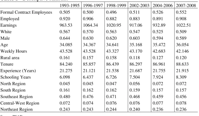
Table 1 - Descriptive statistics

1993-1995 1996-1997 1998-1999 2002-2003 2004-2006 2007-2008

Formal Contract Employees 0.505 0.500 0.496 0.511 0.526 0.552

Employed 0.920 0.906 0.882 0.883 0.891 0.908

Earnings 963.53 1064.34 1020.95 917.06 932.89 1022.51

White 0.567 0.570 0.563 0.547 0.525 0.509

Male 0.644 0.630 0.620 0.603 0.594 0.589

Age 34.085 34.367 34.641 35.168 35.472 36.054

Weekly Hours 43.528 43.528 43.327 43.170 42.683 42.146

Rural area 0.161 0.157 0.158 0.118 0.127 0.120

Tenure 84.240 85.857 86.439 86.297 86.961 88.633

Experience (Years) 21.275 21.121 21.538 21.687 21.755 21.915

Schooling Years 6.098 6.437 6.726 7.504 7.924 8.309

North Region 0.045 0.045 0.047 0.056 0.072 0.072

South Region 0.161 0.162 0.162 0.159 0.157 0.157

Southeast Region 0.480 0.476 0.471 0.468 0.459 0.456

Central-West Region 0.072 0.074 0.076 0.076 0.077 0.078

Northeast Region 0.243 0.243 0.244 0.240 0.236 0.236

Source: PNAD

(13)

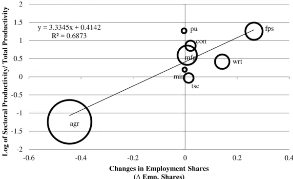
Figure 1 – Correlation between Sectoral Productivity and Changes in Employment

Shares in Brazil (1950-2005)

Source: Timmer and de Vries, 2009

Notes: Size of circles represents employment shares in the initial year.

The line represents fitted values of a linear regression of changes in sectoral productivity by changes in employment shares.

Abbreviations: (agr) Agriculture, (min) Mining, (mfg) Manufacturing, (pu) Public Utilities, (con) Construction, (wrt) Wholesale Trade, (tsc) Transport and Communication, (fps) Financial and Personal Services

We then present some evidence regarding the pattern of structural change in Brazil from 1950 to 2005, by breaking this timeframe down into several different periods. Figure 1 shows that for the whole period, Brazil experienced a classical structural change, as there is a positive correlation (regression coefficient=3.33; R2=0.68; n=8) between sector productivity and changes in employment shares. In other words, during this period of more than 50 years, the labor force migrated to more productive sectors. agr min mfg pu con wrt tsc fps y = 3.3345x + 0.4142

R² = 0.6873

-2 -1.5 -1 -0.5 0 0.5 1 1.5 2

-0.6 -0.4 -0.2 0 0.2 0.4

L og of S e c tor al P r od u c ti vi ty/ T ot al P r od u c ti vi ty

Changes in Employment Shares

(14)

Figure 2 - Correlation between Sectoral Productivity and Changes in Employment

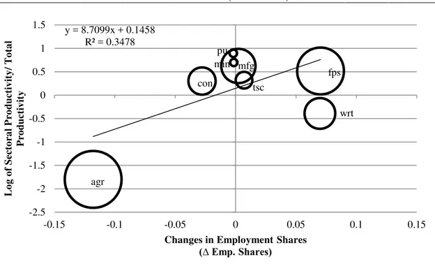
We can see that the correlation between sector productivity and changes in employment shares became progressively weaker as time passed. In fact, rapid inspection of Figures 3 to 5, that present disaggregated evidence for the periods 1965-79, 1980-94 and 1995-2005, reveals that the fitted line gets closer to a null-slope line for more recent years.

agr min mfg pu con wrt tsc fps y = 17.259x + 0.4142

R² = 0.7447

-2 -1.5 -1 -0.5 0 0.5 1 1.5 2

-0.12 -0.1 -0.08 -0.06 -0.04 -0.02 0 0.02 0.04 0.06 0.08

L og of S e c tor al P r od u c ti vi ty/ T ot al P r o d u c ti v ity

Change in Employment Shares

(15)

Figure 3 - Correlation between Sectoral Productivity and Changes in Employment

McMillan and Rodrik (2011) estimated the components of Equation (3) and showed that most of productivity gains in Latin America from 1990 to 2005 were due to the within effect and came little from the structural change component. Their interpretation of the findings is that the region was suffering from a reverse structural change, during which the labor force migrated from the most to the least productive activities. This interpretation is not necessarily true for the Brazilian case. In fact, informality, which is associated with low productivity jobs, and the percentage of workers who live in rural areas have slightly decreased over the period (see Table I).

R² = 0.733

-2 -1.5 -1 -0.5 0 0.5 1 1.5 2

-0.25 -0.2 -0.15 -0.1 -0.05 0 0.05 0.1 0.15 0.2

Change in Employment Shares

(16)

Finally, but not less interestingly, we note that in all figures, the manufacturing sector is not, as was customarily thought, the highest productivity sector. This sector was also not the main attractor of the labor force. For all years, the service sectors, including the Financial and Personal Services or the Public Utilities sector, were the most productive. At the same time, these sectors mostly attracted displaced workers from rural areas. Indeed, employment shares in the Manufacturing sector have remained basically constant for the entire period.

agr

min mfg pu

con

wrt tsc

fps y = 8.7099x + 0.1458

R² = 0.3478

-2.5 -2 -1.5 -1 -0.5 0 0.5 1 1.5

-0.15 -0.1 -0.05 0 0.05 0.1 0.15

(17)

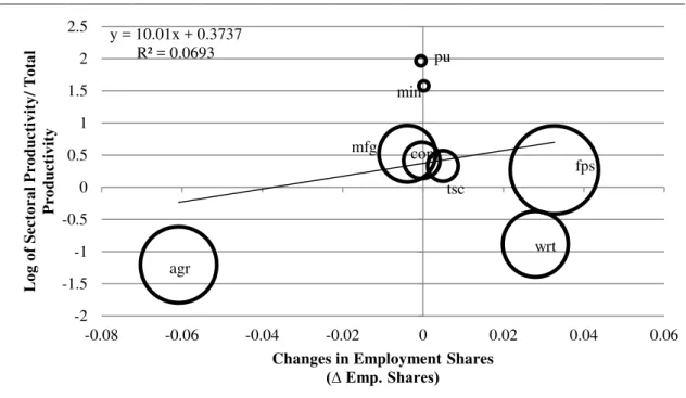
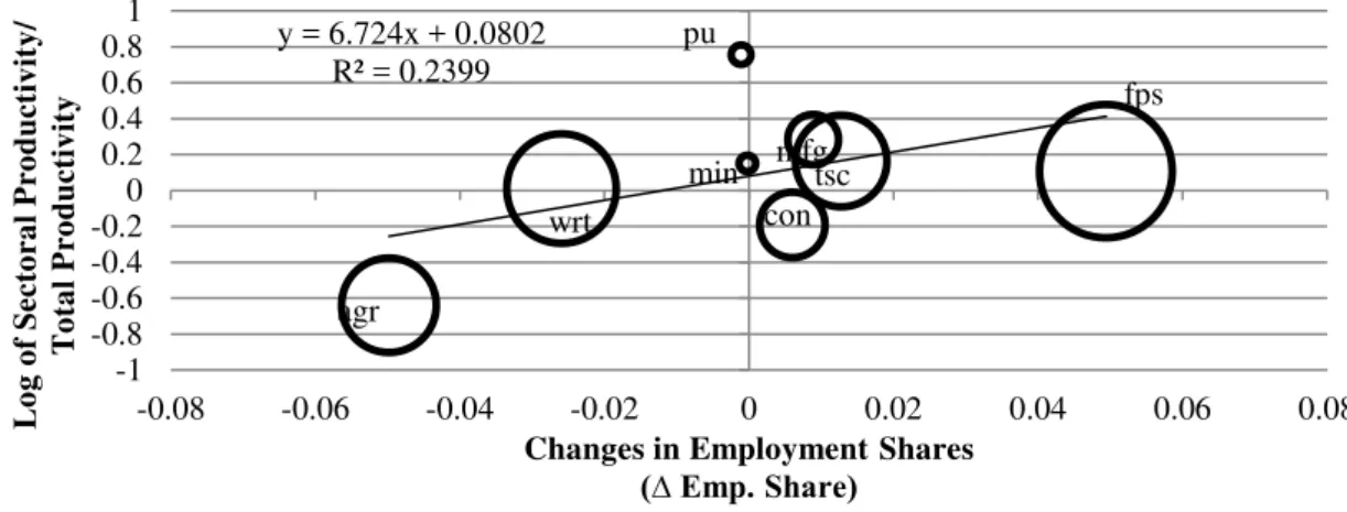
Figure 6 provides evidence for the period from 1993-2008 using PNAD data. In this figure, we can see a consistency in our results, when compared to Figure 5. Even changing the data set, we can see that there is a positive, but very weak correlation (regression coefficient is 6.72, R2=0.24 and n=8) between sector productivity and changes in employment shares for that period.

R² = 0.0693

-2 -1.5 -1 -0.5 0 0.5 1 1.5 2 2.5

-0.08 -0.06 -0.04 -0.02 0 0.02 0.04 0.06

(18)

Shares in Brazil (1993/95-2007/08)-PNAD

Source: PNAD

The decline in the ‘structural change’ effect over time might serve as evidence that policies, like the Brazilian ISS, that protected some specific sectors have lost effectiveness when compared to the first several post-World War II years. Although the agriculture sector still employs almost 20 percent of the labor force, it is no longer a net supplier of workers. Therefore, in more recent years, the most effective policies oriented at promoting economic growth in an emerging economy like Brazil, a country that has already suffered a ‘structural change,’ seem to be policies oriented at increasing within-sector productivity for all economic within-sectors.

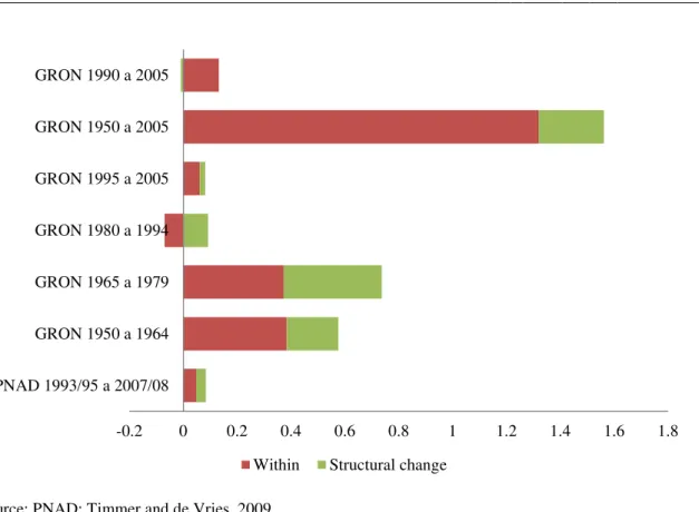
This interpretation is endorsed by empirical evidence. We performed an estimation of Equation (3) for several periods. Figure 7 graphically summarizes our findings. For the entire period from 1950-2005, the within-sector effect was four times larger than the structural change effect. The two effects reached about the same magnitude only for the periods of 1950-1964 and 1965-1979. The period from 1980 to 1994, which includes the end of the autarkic regime, was the worst period in terms of productivity growth. In fact, during those years the Brazilian economy experienced a within-sector productivity decrease and mediocre overall growth. Only after the

agr

min mfg

pu

con wrt

tsc

fps y = 6.724x + 0.0802

R² = 0.2399

-1 -0.8 -0.6 -0.4 -0.20 0.2 0.4 0.6 0.81

-0.08 -0.06 -0.04 -0.02 0 0.02 0.04 0.06 0.08

L og of S e c tor al P r od u c ti vi ty/ T o ta l P r o d u c ti v ity

(19)

consolidation of the trade liberalization process, did the Brazilian economy recover its productivity growth. For the period between 1995 and 2005, most of the growth was due to increases in the within-sector component of productivity changes.

As can also be noted in Figure 7, the period analyzed by McMillan and Rodrik (2011), ranging from 1990 to 2005, is the one in which there was no structural change. All observed changes in productivity came from the within-sector component. One possible explanation for the growth led by the within effect, is that the economy became more exposed to international competition during this period. Muendler (2004) also observed evidence regarding this pattern. The author verified a modest (but positive) impact of trade liberalization on the elimination of inefficient firms and an increase in productivity.

Figure 7 - Decomposition of productivity growth by period and database

Source: PNAD; Timmer and de Vries, 2009

Using PNAD data, we investigate the main forces driving structural and within sector changes in productivity for the period 1993 to 2008. Tables 2 through 5 present some information, by economic sector, from 1993-95 and 2007-2008.

-0.2 0 0.2 0.4 0.6 0.8 1 1.2 1.4 1.6 1.8

PNAD 1993/95 a 2007/08 GRON 1950 a 1964 GRON 1965 a 1979 GRON 1980 a 1994 GRON 1995 a 2005 GRON 1950 a 2005 GRON 1990 a 2005

(20)

Table 2 relates the average monthly earnings by economic sector. We can see that workers in the Agriculture and Mining sectors have encountered the highest increases in earnings for that period. On the other side of the spectrum, workers in the Public Utilities sector faced the greatest losses. A possible explanation for this phenomenon is related to sectoral employment shares. As Agriculture experienced a sharp decrease in its employment shares, it is plausible that the productivity within the sector increased, either as a cause or as a consequence of this reduction. This increase in productivity is captured in Table 2. Finally, it is worth noting the 12 percent earnings growth of the Financial and Personal Services sector. Interestingly, this sector, unlike Agriculture, increased its employment shares during the same period.

Table 2 - Average monthly earnings by sector

Sectors 1993-1995 2007-2008 Difference (in p.p.)

Agriculture, Forestry and Fishing 508.586 598.487 17.68

Mining and Quarrying 1120.166 1539.344 37.42

Manufacturing 1135.916 1029.030 -9.41

Construction 794.869 819.726 3.13

Wholesale and Retail Trade, Hotels and Restaurants 974.233 978.760 0.46

Public utilities 2052.403 1628.540 -20.65

Transport, Storage and Communication 1278.819 1202.321 -5.98

Financial and Personal Services 1073.234 1199.739 11.79

Source: PNAD

Note: Earnings are measured in 2008 Reais

Table 3 offers an explanation of reasons for the changes in sectoral earnings. In all sectors, workers have acquired more years of schooling than had been obtained 20 years ago. However, we note that for the sectors whose increase in years of schooling was below overall growth (36 percent), earnings either fell or did not grow. Agriculture and Mining faced substantial increases in the levels of schooling received by their labor force, 60 percent and 72 percent respectively, and earnings substantially increased. Positive selection into these sectors is therefore, the most likely explanation for our findings.

(21)

were Manufacturing, Public Utilities and Transport, Storage and Communication. Not surprisingly, these sectors faced a decrease in earnings and the years of schooling of their labor force increased below that of the national average.

Table 3 - Average years of schooling by sector

Manufacturing 6.426 8.430 31.19

Construction 4.224 5.923 40.22

Public utilities 8.610 9.585 11.32

Transport, Storage and Communication 6.433 8.364 30.02

Source: PNAD

Table 4 - Percentage of formal contract workers by sector

Manufacturing 0.752 0.703 -4.90

Financial and Personal Services 0.626 0.620 -0.60

Source: PNAD

Informality can be understood as a barrier to creating longer capital-work relationships. Thus, sectors with higher levels of informality also have larger turnover rates. Thus, workers in these sectors are accumulating less experience or specific human capital. This might explain the correlation between informality decreases and earnings increase for the sectors being analyzed.

(22)

technological change, which expelled workers by adopting capital intensive technologies. This explanation is very plausible in regards to Agriculture. In fact, this sector had a decrease in employment shares of five percentage points, but an increase of 18 percent in real earnings for the period.

Table 5 - Employment rate by economic sector and period – PNAD

Agriculture, Forestry and Fishing 0.164 0.114 -4.98

Mining and Quarrying 0.005 0.005 -0.02

Wholesale and Retail Trade, Hotels and Restaurants 0.219 0.194 -2.59

Source: PNAD

For other sectors, we see no obvious relationship between earnings and employment share changes. For example, Public Utilities, which faced a substantial loss in earnings, did not suffer any change in terms of employment shares throughout the period. Another important change was the employment growth of Financial and Personal Services. For this sector, employment shares increased by about five percentage points and earnings grew by about 12 percent.

(23)

Figure 8 - Employment shares for selected sectors

Notes: The orange rectangle represents the period of trade liberalization

We reconcile our findings with the stylized fact observed in McMillan and Rodrik (2011), by emphasizing the fact that in an emerging economy like Brazil, structural changes have become much less important to explaining productivity growth than in the past. One possible explanation for this is that the country has already become industrialized, and the economy’s exceeding labor force that historically migrated from Agriculture has found other destinations. Some potential destinations, as shown in Table 2, present better perspectives, in terms of future earnings, than in the Manufacturing sector. This indicates that productivity growth has spilled over to other sectors, mainly as a result of increases in the human capital of individual workers.

Conclusions and policy discussion

We presented evidence that Brazil has suffered a structural change in its economy since the early 1950s, as was recently defined by McMillan and Rodrik (2011). Employment shares from the least productive sectors have fallen and increased in the most productive ones. However, by breaking this event down into shorter periods,

0 0.1 0.2 0.3 0.4 0.5 0.6 0.7

1950 1955 1960 1965 1970 1975 1980 1985 1990 1995 2000 2005

(24)

we have shown that structural change was only important until the 1970s. By this period, the country had dramatically increased the participation of its manufacturing sector in the overall GDP to 45 percent, according to the Brazilian Bureau of Labor and Statistics (IBGE). The scope for continuous and long-term structural change had lost momentum. In fact, we argue that policies that tried to invert this natural trend were unsuccessful, and the early years of the 1980s can serve as witness reflecting those efforts.

The key to promoting productivity growth in the Brazilian economy after the 1970s seems to have been investing in within-sector productivity growth. More efficient firms and technologies, and workers with higher levels of schooling explain part of the success of the Brazilian economy in the 2000s. This movement towards efficiency began in the late 1980s with the Democratic Regime and reached its peak during the late 1990s.

Descriptive data suggests that the trade liberalization of the 1990s did not have an impact on structural change, but was probably the major reason for productivity increases within sectors. Muendler (2004) provides some evidence for these productivity gains through the channel of competitive push.

During the 2000s, policy makers were able to shift attention towards another important by-product of the country’s rapid process of urbanization and industrialization: high levels of income inequality. Thus, policies oriented at mitigating economic inequalities were put into action, sometimes at the expense of efficiency. Interestingly, as has been pointed out since the seminal work by Langoni (2005) and Fishlow (1972), rapid industrialization was the major cause of increases in earnings inequality. Also of note, Gonzaga et al. (2006) showed that trade liberalization had an important impact on decreasing the schooling wage gap, which is a relevant source of wage inequality in the country.

(25)

an important channel that has driven overall productivity growth to be positive. In this context, the recent setback observed in the process of trade liberalization with a rise in tariffs for cars, electronics, and other manufactured goods may no longer be justified as a growth-enhancing policy.

Notes

1. Sao Paulo School of Economics - FGV, C-Micro - FGV, and IZA. Corresponding author. E-mail:

sergio.firpo@fgv.br.

2. Sao Paulo School of Economics - FGV, C-Micro - FGV.

3. Calculating productivity using Groninger Table and PNAD for 1995 to 2005 (excepting 2000 and

2001) we found 55% Pearson correlation coefficient. Regressing productivity coefficient calculated from (1) by productivity calculated from (2) we found a coefficient of 2.25 and a standard deviation of 0.031. This presents some evidence that both measures of productivity we use in the paper are positive correlated.

4. In Figure 3 regression coefficient is 8.10, R2_{=0.73 and n=8. In Figure 4 regression coefficient is 8.70,}

R2_{=0.34 and n=8. In Figure 5 regression coefficient is 10.01, R}2_{=0.07 and n=8.}

References

Abreu, Marcelo de Paiva, 2004. “The political economy of high protection in Brazil before 1987," Special Initiative on Trade and Integration, Working paper SITI-08a.

_____, 2004. “Trade Liberalization and the Political Economy of Protection in Brazil since 1987," Special Initiative on Trade and Integration, Working paper SITI-08b, 2004.

Baer, Werner & Kerstenetzky, Isaac. (1964): Import Substitution and Industrialization in Brazil. The American Economic Review, Vol. 54, No. 3, pp. 411-425.

Baer, W., Fonseca, M. A. R., and Guilhoto, J. J. M. (1987). Structural changes in Brazil’s industrial economy, 1960 – 80. World Development, 14, 275 – 286.

(26)

Fagerberg J (2000) Technological progress, structural change and productivity growth:

a comparative study. Working paper N˚ 5/2000, Centre for Technology, Innovation and Culture, University of Oslo.

Ferreira, F. H. G., Phillippe G. Leite, and Matthew Wai-Poi, 2007. “Trade Liberalization, Employment Flows, and Wage Inequality in Brazil," World Bank Policy Research Working Paper (4108).

Fishlow, A., 1972, “Brazilian Size Distribution,” The American Economic Review, 62

(2), 391-402.

Gonzaga, G., N. Menezes-Filho and C. Terra, 2006, “Trade liberalization and the evolution of skill earnings differentials in Brazil,”Journal of International Economics,

68, 345-367.

Helpman, E. and Paul Krugman (1985). Market Structure and Foreign Trade: Increasing Returns, Imperfect Competition and the International Economy. Cambridge: MIT Press.

Kovak, Brian, 2011. “Local labor market effects of Trade Policy: evidence from Brazilian liberalization,”

Kume, Honorio, Guida Piani, and Carlos Frederico Bráz de Souza, 2003. “A Política Brasileira de Importação no Período 1987-1998: Descrição e Avaliação," in Carlos Henrique Corseuil and Honorio Kume, eds., A Abertura Comercial Brasileira nos Anos 1990: ImpactosSobre Emprego e Salário, Rio de Janiero: MTE/IPEA, chapter 1, pp. 1-37.

Langoni, Carlos Geraldo, 2005, “Distribuição da renda e desenvolvimento econômico do Brasil,” FGV Editora, Rio de Janeiro.

McMillan, Margaret S. & Rodrik, Dani, 2011. "Globalization, Structural Change and Productivity Growth," NBER Working Papers 17143, National Bureau of Economic Research, Inc

(27)

(28)

Appendix A: Other descriptive statistics by sectors

Table A.1 - Percentage of whites by sector

Sectors

1993-1995

2007-2008

Difference (in p.p.)

Construction 0.477 0.398 -7.90

Source: PNAD

Table A.2 - Percentage of males by sector

Source: PNAD

Table A.3 - Average age by sector

Construction 34.991 37.977 8.53

(29)

Table A.4 - Average tenure (months) by sector

Manufacturing 63.700 74.521 16.99

Construction 73.617 93.171 26.56

Source: PNAD

Table A.5 - Average experience (years) by sector

Construction 22.638 24.495 8.20

Source: PNAD

Table A.6 - Percentage of workers in North region by sector

(30)

Table A.7 - Percentage of workers in South region by sector

Source: PNAD

Table A.8 - Percentage of workers in Southeast region by sector

Source: PNAD

Table A.9 - Percentage of workers in Central-West region by sector

(31)

Table A.10 - Percentage of workers in Northeast region by sector

(32)

Appendix B: Decomposition of informality

Here we decompose the informality growth (variation in the percentage of informal contract workers) by the following equation:

�� = ��− �� =∑ ��9_� ��.+∑ ��9_� ��. (B.1)

where Ejt is the share of industry j's employment by total employment at time t, ijt is the

share of informal workers by total employment in industry j, Ej.=0.5(Ejt+Ejτ), and

ij.=0.5(ijt+ijτ). The first term of the decomposition is the “within effect” and represents

changes in informality on each sector, keeping employment shares constant. The second is the “between effect” and it denotes changes in informality due to the migration of workers across sectors, keeping the rate of informality of each sector constant.

Figure B.1 presents the decomposition for the period 1993 to 2008. The figure suggests that greatest decrease in informality observed in the period is due to the movement of the labor force to the direction of sectors with higher rates of formality.

Figure B.1 - Decomposition of informality growth - 1993/95-2007/08

Source: PNAD

-0.06 -0.05 -0.04 -0.03 -0.02 -0.01 0