Evaluation of snow data assimilation using the ensemble Kalman filter for seasonal streamflow prediction in the western United States

(1)

Hydrol. Earth Syst. Sci., 21, 635–650, 2017 www.hydrol-earth-syst-sci.net/21/635/2017/ doi:10.5194/hess-21-635-2017

Evaluation of snow data assimilation using the ensemble

Kalman filter for seasonal streamflow prediction in

the western United States

Chengcheng Huang1,2, Andrew J. Newman2, Martyn P. Clark2, Andrew W. Wood2, and Xiaogu Zheng1 1_{College of Global Change and Earth System Science, Beijing Normal University, Beijing, China}

2_{National Center for Atmospheric Research, Boulder, CO 80301, USA} Correspondence to:Andrew J. Newman ([email protected])

Received: 21 April 2016 – Published in Hydrol. Earth Syst. Sci. Discuss.: 4 May 2016 Revised: 19 December 2016 – Accepted: 20 December 2016 – Published: 31 January 2017

Abstract. In this study, we examine the potential of snow water equivalent data assimilation (DA) using the ensem-ble Kalman filter (EnKF) to improve seasonal streamflow predictions. There are several goals of this study. First, we aim to examine some empirical aspects of the EnKF, namely the observational uncertainty estimates and the observation transformation operator. Second, we use a newly created en-semble forcing dataset to develop enen-semble model states that provide an estimate of model state uncertainty. Third, we ex-amine the impact of varying the observation and model state uncertainty on forecast skill. We use basins from the Pacific Northwest, Rocky Mountains, and California in the west-ern United States with the coupled Snow-17 and Sacramento Soil Moisture Accounting (SAC-SMA) models. We find that most EnKF implementation variations result in improved streamflow prediction, but the methodological choices in the examined components impact predictive performance in a non-uniform way across the basins. Finally, basins with rel-atively higher calibrated model performance (> 0.80 NSE) without DA generally have lesser improvement with DA, while basins with poorer historical model performance show greater improvements.

1 Introduction

In the snow-dominated watersheds of the western US, spring snowmelt is a major source of runoff (Barnett et al., 2005; Clark and Hay, 2004; Singh and Kumar, 1997; Slater and Clark, 2006). In such basins, the initial conditions of the

basin, primarily in the form of snow water equivalent (SWE), drive predictability out to seasonal timescales (Wood et al., 2005; Wood and Lettenmaier, 2008; Mahanama et al. 2012; Staudinger and Seibert, 2014; Wood et al., 2016). Thus, ter estimates of basin mean initial SWE should lead to bet-ter seasonal streamflow predictions (Arheimer et al., 2011; Clark and Hay, 2004; Slater and Clark, 2006; Wood et al., 2016). For various reasons (e.g., the uncertainty in model pa-rameters, forcing data, model structures), simulated SWE in hydrological models can be very different from reality (Pan et al., 2003). Fortunately, a variety of snow observations (in-cluding point gauge and spatial satellite data) contain valu-able information (Andreadis and Lettenmaier, 2006; Barrett, 2003; Engeset et al., 2003; Mitchell et al., 2004; Su et al., 2010; Sun et al., 2004).

(2)

636 C. Huang et al.: Evaluation of snow data assimilation

to estimate the observed SWE state in a watershed of inter-est (e.g., Franz et al., 2014; Jörg-Hess et al., 2015; Slater and Clark, 2006; Wood and Lettenmaier, 2006).

Here, we use the ensemble Kalman filter (EnKF) method for DA using an implementation that allows for seasonally varying estimates of observation and model error variances (Evensen, 1994, 2003; Evensen et al., 2007). The EnKF framework has been successfully implemented in research basins in several previous studies (Clark et al., 2008; Franz et al., 2014; Moradkhani et al., 2005; Slater and Clark, 2006; Vrugt et al., 2006). The EnKF provides an objective analyt-ical framework to optimize the update of model states based on observed values and their corresponding uncertainties. While the EnKF approach has a formal theory, its overall objectivity in an application (contrasting with an arbitrary DA approach such as direct insertion) nonetheless depends on several methodological choices that are often empirical when applied to SWE DA.

Following Slater and Clark (2006), this study uses two slightly different approaches to estimate ensemble SWE ob-servations with point gauge SWE data from surrounding gauge sites for study basins. When using calibrated hydro-logic modeling systems, model SWE states may exhibit sys-tematic biases from observed SWE estimates for a number of reasons – e.g., all hydrologic models must simplify real watershed physics and structure, and model parameter es-timation (calibration) may result in SWE behavior that in part compensates for forcing or model errors (e.g., Slater and Clark, 2006). Therefore, transformation of snow obser-vations to model space is needed before they are used to up-date the model states to ensure that the model ingests SWE estimates that are as close to unbiased, relative to the model climatology, as possible. We explore two variations on an ap-proach using cumulative density function (CDF) transforma-tions of observatransforma-tions to model space (following Wood and Lettenmaier, 2006, among others). Additionally, we under-take a sensitivity analysis to highlight the importance of ro-bust observations and model uncertainty estimates. We focus on the impacts of updates made just once per snow accumula-tion season, noting that an important choice that is not exam-ined as a result is the selection of DA dates and frequency. For a given generally optimal selection of the EnKF ap-proach, the ensemble streamflow prediction (ESP) approach is used to test the impact of SWE DA on subsequent stream-flow forecasts.

For context, operational seasonal streamflow forecasts in the US currently do not use formalized DA. If the initial states of the model are suspected to contain error (He et al., 2012), DA is performed through subjective forecaster inter-vention. Manual adjustments (termed MODs; e.g., Ander-son, 2002) to model states (e.g., SWE) are applied repeatedly throughout the water year, and particularly before initializing seasonal forecasts. This manual nature of the correction hin-ders the ability to scale up DA procedures to many basins, to benchmark DA performance, and quantify improvements

Figure 1.Location of nine case basins in the western United States (US) and SWE gauge sites.

to the forecast system, as skill depends on the forecaster’s experience (Seo et al., 2003).

The central motivating aim of this study is thus to as-sess the potential benefits of objective, automated SWE DA against a reference model configuration to identify forecast improvement opportunities. We apply the EnKF DA ap-proach to nine river basins in the western US that have a range of basin features and environmental conditions, over a period of multiple decades. This experimental scope differs from many previous studies that focus on one or two basins (e.g., Clark et al., 2008; Franz et al., 2014; He et al., 2012; Moradkhani et al., 2005) or assess DA performance over shorter periods. We also use ensemble simulations driven by a new probabilistic forcing dataset (Newman et al., 2015b, c) as a basis for estimating model SWE uncertainty, in contrast to prior studies that relied on more arbitrary distributional assumptions. This range of basins permits us to explore the question of “In what types of basins might automated SWE DA improve seasonal streamflow forecasts?”.

(3)

C. Huang et al.: Evaluation of snow data assimilation 637

Table 1.Basin features of nine case basins.

Region Basin ID Elevation Minimum Maximum DA date Basin area Slope Forest Basin name (m) elevation elevation (km2) (m km−1) fraction

(m) (m)

14 09081600 3092.15 2050 4250 1 April 436.88 150.58 0.61 Crystal River 14 09352900 3459.15 2450 4250 1 April 187.74 156.09 0.52 Vallecito Creek 17 13023000 2468.57 1750 3450 1 March 1163.72 98.51 0.68 Greys River 17 12147600 998.25 550 1650 1 April 16.07 159.37 1 SF Tolt River 17 13235000 2077.16 1150 3250 1 April 1158.47 126.25 0.86 SF Payette River 17 14158790 1210.48 750 1750 15 March 40.76 116.44 1 Smith River 16 10336645 2180.92 1850 2650 1 April 20.09 118.27 0.71 General Creek 16 10336660 2188.08 1850 2650 1 April 32.46 83.46 0.79 Blackwood Creek 18 11266500 2576.54 1150 3950 1 April 836.15 140.18 0.67 Merced River

model mean SWE; and (3) sensitivity analyses of the relative size of observed and model error variance.

The following sections discuss the study basins and datasets, and the model and EnKF DA approach, before the presenting study results and discussion, and a summary.

2 Study basins and data

In this study, nine basins across the western US are selected for SWE DA evaluation. They are in the Pacific Northwest, California (Sierra Nevada Mountains), and central Rocky Mountains. We focus on these three areas as they span a range of snow accumulation and melt conditions of the west-ern US and are in areas with active seasonal streamflow pre-diction and water resource management. We do not examine rain-driven low-lying basins because they do not have signifi-cant SWE contributions to runoff. The locations of the basins and nearby SWE gauge sites are shown in Fig. 1, illustrat-ing that all of the study watersheds have SWE measurements distributed in and/or around the basins. The main features of these basins are shown in Table 1. The basin areas range from 16 to 1163 km2, and the mean elevations of the basins range from 998 to 3459 m with a large spread in basin mean slopes (as estimated from a fine-resolution digital elevation model) and forest percentage.

Two sources of SWE observations are used in this study: (1) the widely used snow telemetry network (SNOTEL) for Natural Resources Conservation Service (NRCS), which covers most of the western US (NRCS, https://www.wcc. nrcs.usda.gov/snow/); and (2) the California Department of Water Resources (DWR, denoted as CADWR sites here-after), which maintains a snow pillow network for California (CADWR, http://cdec.water.ca.gov/snow/). The SWE data from CADWR sites have frequent missing data and some un-realistic extreme values; thus, extensive manual quality con-trol was required before using the CADWR data in the study.

3 Methodology

3.1 Models and calibration

The Snow-17 temperature index snow model is coupled to the Sacramento Soil Moisture Accounting (SAC-SMA) con-ceptual hydrologic model (Anderson, 2002, 1973; Burnash and Singh, 1995; Burnash et al., 1973; Franz et al., 2014; Newman et al., 2015a) to simulate streamflow in this study. This model combination has been in operational use by US National Weather Service (NWS) River Forecast Centers (RFCs) since the 1970s (Anderson, 1972, 1973). The Snow-17 model is a conceptual snow pack model that employs an air temperature index to partition precipitation into rain and snow and parameterize energy exchange and snowpack evo-lution processes. The only required forcing inputs are near-surface air temperature and precipitation. The output rain-plus-snowmelt (RAIM) time series from Snow-17 is part of the forcing input of the SAC-SMA model. SAC-SMA is a conceptual hydrologic model that uses five moisture zones to describe the movement of water through watersheds. The required forcing input is the potential evaporation and the surface water input from Snow-17.

(4)

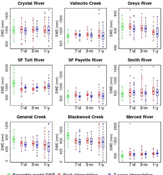
Figure 2.Box plots of ensemble model SWE and estimated ensemble SWE observations for the nine case basins on the data assimilation date in 2004 for three window lengths – 7 days (7-d), 3 months (3-m), and 1 year (1-y).

the ensemble model states serves as the estimate of model uncertainty. Because this method estimates SWE uncertainty without also considering sources other than forcing input uncertainty, and therefore may underestimate model uncer-tainty in initial SWE (e.g., Franz et al., 2014), we also in-clude a sensitivity analysis to explore the sensitivity of DA results to variations in the estimated observation and model uncertainty magnitudes.

3.2 Generating ensembles of estimated observed watershed SWE

Since the SWE gauge observations are point measurements that do not represent the watershed mean conditions and have observation error, observation uncertainty needs to be ro-bustly estimated to ensure reasonable DA performance. In

(5)

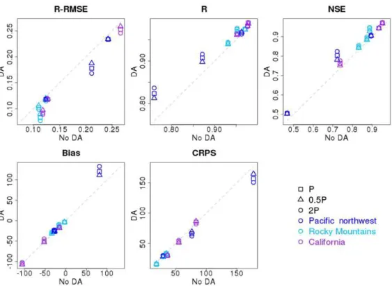
Figure 3.Evaluation metrics for April–July ensemble mean streamflow from the percentile-based interpolation method for the nine case basins using perfect forcing. The verification metrics from upper left to lower right are as follows: R-RMSE is the relative (normalized) root mean squared error,Ris the linear (Pearson) correlation coefficient, NSE is the Nash–Sutcliffe efficiency, bias is the same as mean error, and CRPS is the continuous ranked probability skill score.

3.2.1 Percentile interpolation

First, the non-exceedance percentilep_yo(k)of each SWE ob-servation (obob-servation-based values noted with superscript o) at gauge sitekon the DA date in yeary is calculated based on its rank, or percentile, within a sample of all SWE obser-vations in all years at the same site within a time window of ±ndays centered on the date of the observation in each year. Then, we use the percentiles to do linear regression on geo-graphic features latitude, longitude, and elevation to estimate the SWE percentile for the target basin:pˆo_y, where the hat indicates the basin mean estimate. By LOO cross validation, the interpolation error of the linear regression is estimated as

ˆ

eo_y. We sample from normal distributionN (pˆo_y,ˆeo_y)to get the ensemble percentiles { ˆpo_y(j )}, wherej=1, . . . , 100 repre-sents the ensemble member.

Finally, we take the correspondingpˆ_yo(j )percentile from the full ensemble model SWE within the time window of±n days centered on the DA date each year in all years, denoted as Sˆ_yf(j ). The final ensemble SWE observations on the DA date in yearyfor the target basin are{ ˆS_yf(j )}, wherej =1, . . . , 100.

3.2.2 Zscore interpolation

First, we use the observed SWE at gauge sitek on the DA date in yearyto calculate theZscore:

Zscorey(k)=

S_yo(k)−So(k)

σ (So_(k)) , (1)

whereSo_(k)_and_{σ (S}o_(k))_{are the long-term mean and} stan-dard deviation of a sample of all non-zero SWE observations at the same site within a time window of±ndays centered on the date of the observation, respectively. Here, we use the Z score in the linear regression and again use LOO cross validation to estimate the mean and interpolation error of the Zscore for a target basin. Then, we sample from the normal distribution to get ensembleZscores for the target basin, de-noted as{ ˆZscoreo

y(j )}, wherej =1, . . . , 100 represents the

ensemble member. Finally, we use the following equation to transformZscore back to SWE values:

ˆ

S_yo(j )= ˆZscore(j )o_y×σSf(k)+Sf(k), (2)

whereSf_(k)_and_{σ S}f_(k)

(6)

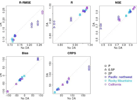
Figure 4.Evaluation metrics for April–July ensemble mean streamflow from theZscore interpolation for the nine case basins using perfect forcing. The verification metrics from upper left to lower right are as follows: R-RMSE is the relative (normalized) root mean squared error,Ris the linear (Pearson) correlation coefficient, NSE is the Nash–Sutcliffe efficiency, bias is the same as mean error, and CRPS is the continuous ranked probability skill scores.

observations on the DA date in yearyfor the target basin are { ˆS_yo(j )}, wherej=1, . . . , 100.

Both percentile and Z score transformations normalize the original SWE values to decrease their spatial variability (Slater and Clark, 2006; Wood and Lettenmaier, 2006). The latter ensures the ensemble observations have the same mean as the ensemble model SWE and the variance of ensemble observations is proportional to ensemble model SWE vari-ance. The former emphasizes the shape of the observation time series. SWE observations in and near a watershed but at different elevations may have greatly varying values, but their percentile andZscore statistics will show reduced vari-ation because they arise from similar relative weather condi-tions with respect to condicondi-tions in other years. Using normal-ized statistics significantly reduces the interpolation uncer-tainty and systematic biases relative to the watershed’s SWE climatology.

3.3 EnKF approach and experimental design

For evaluating the relative performance of DA and for re-initializing the soil moisture of DA runs at the beginning of each water year (WY), an open-loop or “control” retrospec-tive simulation (denoted No DA) is performed using the cal-ibrated model parameters with ensemble forcing data. This control run is one continuous simulation per ensemble

mem-ber for the entire hindcasting and evaluation period (1981– 201X) for each basin, where “201X” is the last simulation year available between 2010 and 2014. Because this study focuses on assessing variations in methodological aspects of the DA approach rather than differences in performance throughout a forecasting season, we apply DA updates only once per year, using the date on which the SWE correlation with future runoff is highest for the study basin, but no later than 1 April, a common date for initiation of spring seasonal runoff forecasts.

The EnKF method used in this study is a time-discrete forecast and linear observation system described by two rela-tionships (generally following the notation of Ide et al., 1997 and Wu et al., 2012):

xt_i+₁=M xt_i+ηi, (3) yo_i =h xt_i+εi, (4)

(7)

re-C. Huang et al.: Evaluation of snow data assimilation 641

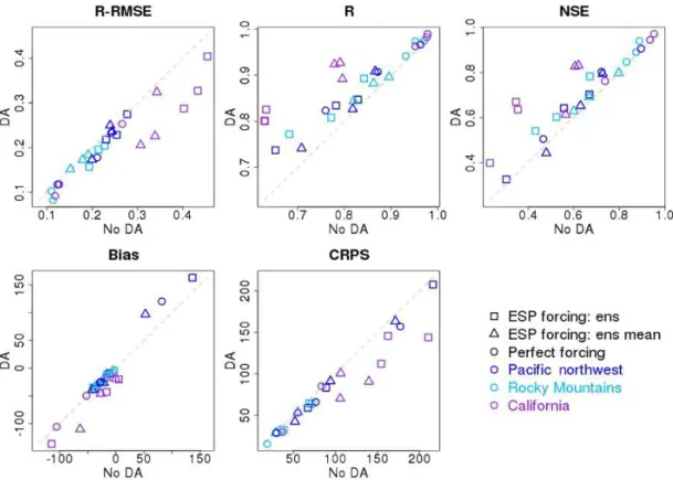
Figure 5.Evaluation statistics of percentile interpolation for the nine case basins with the two variations of ensemble streamflow prediction (ESP) and with perfect forcing data (ens in the legend denotes ensemble). The verification metrics are the same as in Fig. 4.

gard the SWE estimates that have been transformed to model space as observationyas a preprocessing step.

The SWE DA approach is implemented via the following procedure:

1. The watershed model is run once for each ensemble forcing member from the beginning of a WY until the DA date with initial statesx0taken from the retrospec-tive control runs, producing the ensemble forecast states

xf_i. The superscript f denotes forecast.

2. The ensemble analysis states are calculated as follows:

xa_i =xf_i+sihTi

hisihTi +oi −1

di, (5)

where superscript a means analysis,oandsare the ob-served and model simulation error variances (estimated by the variance of ensemble observations and model states, respectively), and the innovation vector (resid-ual) is calculated as

di=yoi −hi

xf_i. (6)

3. The Snow-17 SWE states are updated with the analysis states to use for initialization of forecasts through the end of the WY.

Steps 1–3 are repeated for all WYs available in the hind-cast period (1981–201X). Soil states are re-initialized using the states from the retrospective (No DA) run at the start of every WY (October 1), when there is no SWE. To summa-rize, we calculate an analysis via Eq. (5) and use that analy-sis to update the Snow-17 SWE states. We then run the model with the updated states until the end of the WY.

3.4 Model and observation error variance

(8)

Figure 6.Incremental change in evaluation statistics for ESP and perfect forcing forecasts using percentile-based interpolation for the nine case basins. R is the linear (Pearson) correlation coefficient, NSE is the Nash–Sutcliffe efficiency, and CRPS is the continuous ranked probability skill score.

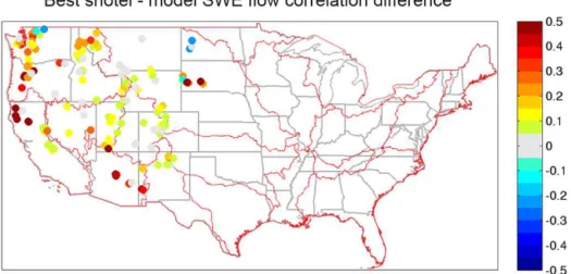
Figure 7.Difference of the rank correlation of SWE and runoff from the best SNOTEL site (of nearest 10) and calibrated model without DA.

3.5 Seasonal ensemble streamflow prediction

Although the impacts of the SWE DA on forecast accuracy can be assessed through verification of post-adjustment sim-ulations using “perfect” future forcing, we demonstrate the performance of SWE DA by initializing seasonal ESP fore-casts for a streamflow forecast product that is widely used in water management, the snowmelt period runoff volume from

(9)

en-C. Huang et al.: Evaluation of snow data assimilation 643

Figure 8.Time series plots for SWE and runoff for the Greys River for water year 1997. Light blue lines indicate individual ensemble member traces. Vertical black dashed line denotes the DA date.

semble by randomly selecting 1 year of the historical ensem-ble forcing data for each historical member of the ESP; and (2) we use all historical years of ensemble mean forcing data for each ESP historical year member, yielding a 30× 100-member ensemble for an ESP based on meteorology from 1981 to 2010 (variations are noted as ens forcing and ens mean forcing, respectively, in subsequent figures discussing ESP results).

3.6 Verification metrics

In this study, five frequently used statistics are calculated for April through July seasonal streamflow volume expressed as runoff (mm) for evaluating the two DA approaches. The bias, correlation coefficient (R), relative root mean squared error (R-RMSE), and Nash–Sutcliffe efficiency (NSE) are based on the ensemble averages. The continuous ranked probabil-ity score (CRPS) is a measurement of error for probabilistic prediction (Murphy and Winkler, 1987). It is defined as the integrated squared difference between the CDF of forecasts and observations:

CRPS=

+∞ Z

−∞ h

Ff(x)−Fo(x)i2dx, (7)

whereFf andFo are CDFs for forecasts and observations of streamflow, respectively. Small CRPS values mean more

Figure 9.Time series plots for SWE and runoff for the south fork (SF) of the Tolt River for water year 1988. Light blue lines indi-cate individual ensemble member traces. Vertical black dashed line denotes the DA date.

accurate forecasts, with a 0 value indicating a perfect forecast accuracy.

4 Results and discussion

4.1 Overall performance in the case basins

(10)

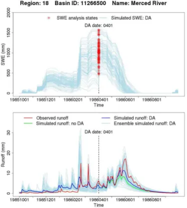
Figure 10. Time series plots for SWE and runoff for the Merced River for water year 1986. Light blue lines indicate individual en-semble member traces. Vertical black dashed line denotes the DA date.

while the 3-month window is only about 120 mm. This is likely due to the more limited sample size for the regression, which can reduce the positive impact of DA performance. For example, the SF Payette River and the Greys River have positive DA impact for both the 7-day and 3-month win-dows but for the 7-day window the positive impact is reduced by roughly half in both basins for most metrics (Tables S1 and S3 in the Supplement). Increased estimated observation variance decreases the weight of the observations in an EnKF approach and thus decreases the impact of the observations. In this study, a 3-month window of SWE observations gen-erally gives the best performance. However, in some basins, a different window length may bring larger improvements. Longer windows mean that the transformation is more statis-tically representative of the long-term model–observation cli-matology. Shorter time windows imply that the model SWE values used for transformation are more relevant to a specific seasonal time period, avoiding aliasing for seasonality, but have much smaller sample sizes and may not properly rep-resent the relationship between model and observation cli-matologies. The window length must be a balance between these two considerations. Therefore, a 3-month window is recommended for both approaches.

The evaluation statistics for simulated streamflow using perfect forcing after DA with ensemble SWE observations estimated by the percentile and Z score interpolation

ap-proaches for the 3-month window are shown in Figs. 3 and 4. They are also compiled in Tables S1–6. In those tables, the second column shows the forecast error variance used to cal-culate analysis states, where “No DA” means the open-loop control run (see Sect. 3.3), and the P, 1/2P and 2P re-fer to the DA runs with the model error variance estimated by 1, one-half, and 2 times the original size of the ensem-ble model variance. Both percentile andZ score interpola-tion approaches exhibit enhanced DA performance among the case basins, indicating that both approaches are effec-tive in adding observation-based information to the model simulations. Overall, using the original model variance esti-mate (caseP), the mean improvement for the percentile in-terpolation method (Zscore method) is a reduction in relative RMSE (R-RMSE) of about 11 % (12 %) and an increase in NSE of 0.03 (0.05). The percentile interpolation andZscore interpolation methods vary in performance across the basins with both performing better in some basins and not others (e.g., percentile interpolation performs slightly better than Z score interpolation in the Greys River using NSE as the evaluation metric (0.94 versus 0.93) and slightly worse than that in the SF Tolt River (0.82 versus 0.88)). Using NSE, percentile interpolation performs better in the Greys River, whileZscore interpolation performs better in the Vallecito, south fork of the Tolt, Merced, and Smith rivers. To the hun-dredth NSE value (0.01), both methods are equivalent in the south fork of the Payette River, and General and Blackwood creeks.

(11)

Figure 11.Scatterplots for seasonal runoff and SWE on the DA date for the Greys River. Black dashed diagonal lines indicate the 1:1 line, while the green lines indicate linear regression fits to data. Perfect forcing results are shown in the top row, while ESP results are in the bottom row.

the basins have a NoDA seasonal runoff NSE of less than 0.8, with an average improvement of 0.05 for the percentile regression and 0.12 for the Z score regression versus 0.03 and 0.05 across all nine basins. Four basins have seasonal runoff NSE values of at least 0.89 and the two DA methods result in minimal improvement, 0.02 for both methods. With a sample size of nine, little statistical significance can be at-tached to these results, but they do suggest DA is more ben-eficial in poorly calibrated basins. Future work will examine the potential for DA based on NoDA (open-loop) model per-formances and the characteristics of nearby observed SWE data.

Figure 5 summarizes the ESP evaluation statistics. For simplicity, only the percentile interpolation approach with a 3-month window is shown without forecast error infla-tion. It shows that for both ESP forcing methodologies used (Sect. 3.5) in all the case study watersheds, SWE DA en-hances seasonal runoff prediction skill, including the prob-abilistic prediction metric CRPS. Again, higher skill NoDA watersheds saw smaller DA improvements. The DA evalua-tion metric improvement increment versus the corresponding NoDA evaluation metric score for the case basins is shown in Fig. 6. The DA improvements in all evaluation metrics have a generally weak negative correlation with NoDA

perfor-mance, which again highlights that better-simulated basins benefit less from SWE DA.

4.1.1 Broader DA potential

(12)

Figure 12.Scatterplots for seasonal runoff and SWE on the DA date for the south fork of the Tolt River. Black dashed diagonal lines indicate the 1:1 line, while the green lines indicate linear regression fits to data. Perfect forcing results are shown in the top row, while ESP results are in the bottom row.

(central basins), model–observation correlation differences are small, potentially indicating reduced DA improvement potential, in agreement with the results seen above.

4.2 Case study analyses

To provide a more in-depth examination of the SWE DA im-pacts to the watershed model states and fluxes, time series of runoff and SWE are shown in Figs. 8, 9, and 10 for three example basins, one for each region (the same figures for the other six basins are included in the Supplement), and for one hindcast year. The feedback from the change of SWE on the DA date to seasonal runoff is readily apparent. Increasing the ensemble model SWE through DA will lead to increased model runoff, and vice versa. For basins with a strong sea-sonal cycle of streamflow (e.g., Greys and Merced rivers), SWE DA may improve daily runoff forecasts in years when seasonal volume forecast improvements are seen, although this is not true in every watershed (e.g., Tolt River). For ex-ample, the daily NSE for the Greys River in 1997 after DA was improved from 0.53 to 0.80 in the perfect forcing exam-ple, and this is via bias reduction, as the daily flow timing is essentially unchanged. In Fig. 9, the NSE of the daily flow prediction of the Tolt River is essentially unchanged (0.54

for DA, 0.53 for NoDA) even though the seasonal volume prediction is improved (1990 mm observed, 1968 mm DA, 1534 mm NoDA). In this case, improvements to bias did not improve NSE as the bias improvements did not improve the squared daily flow differences (e.g., RMSE: 7.76 versus 7.88 for DA versus NoDA).

(13)

Figure 13.Scatterplots for seasonal runoff and SWE on the DA date for the Merced River (same as Fig. 12).

runoff is overestimated), we would expect the SWE incre-ment to be negative in order to decrease the model seasonal runoff (counteract model error) and vice versa. Thus, the ideal results are that the points fall onto different sides of they=0 andx=0 lines (shown as grey dashed lines in this panel); i.e., the points all fall into the second (upper left) and fourth (lower right) quadrants. This is generally the case for our case basins for both perfect and ESP forcing, which again shows that the SWE DA approach is successful in reducing model and forecast error.

For the three basins highlighted here, there are years where the DA SWE increment is not in the second or fourth quad-rants. In these years, the increment decreases subsequent forecast skill. Overall, there are 11 of 28 (39 %), 4 of 24 (17 %), and 12 of 26 (46 %) years for the Greys, Tolt, and Merced rivers where this is the case using perfect forcing. These years generally correspond to small SWE increments relative to that year’s SWE and runoff in all basins, except for 5 years in the Merced River, where the SWE increment is larger than 10 % of that year’s streamflow production and is incorrect. In the Greys River, all incorrect increments are less than 10 % of the observed runoff for that year and also in years where the NoDA runoff error is less than 10 % of observed. A small increment implies that the estimated ob-served and model SWE are very similar, and thus, in years

with small model error, the model SWE climatology closely matches observed climatology after transformation for this basin. Figure 14 highlights an example WY in the Merced River where the SWE increment and runoff error are both negative, indicating that DA increased the model forecast er-ror.

(14)

Figure 14. Time series plots for SWE and runoff for the Merced River for water year 1984. Light blue lines indicate individual en-semble member traces. Vertical black dashed line denotes the DA date.

of El Niño/La Niña signals (not shown) revealed no clear pat-tern with degradation of DA forecast skill.

Lastly, there are years where the NoDA runoff error is large, but the SWE increment is small in all three basins. This is not unexpected, as spring SWE is not perfectly correlated with subsequent runoff. This may also hint at a level of data loss in the EnKF approach, and future work should compare streamflow hindcasts using this type of DA approach with traditional statistical methods using SWE as a primary input. It also suggests that improved model calibration, or in com-bination with model parameter estimation in the EnKF ap-proach (e.g., He et al., 2012), may improve DA performance across all basins, not just the Merced.

5 Summary and conclusions

This study tests variants of EnKF SWE DA approaches in nine case basins in the western US. These basins have sea-sonal runoff representative of basins used for water resource management across the western US and have at least six close SWE gauge sites with 20 or more years of observa-tion history. Two approaches of constructing SWE ensemble observations, percentile andZscore interpolation, are exam-ined in this study in an effort to reduce the spatial variability and decrease the interpolation uncertainty while also

trans-forming the observations to model space (e.g., the range of the model climatology). A 3-month window of SWE obser-vations generally gives the best performance for these two approaches in this study (Figs. 2–4, Tables S1–6). However, in some basins a different window length may bring larger improvements. A suitable window length needs to include sufficient samples for transformation as well as including the most relevant samples (i.e., a specific seasonal time period). Sensitivity analyses of model uncertainty impacts on DA per-formance suggest that either the forcing-alone-based estima-tion of model errors underestimates the total model error variance, or the observed SWE error estimation approaches (interpolation plus the SWE regression) tend to overestimate observation uncertainty, or both (Figs. 3–4, Tables S1–6). Fu-ture work should examine this in more detail, as this work clearly indicates that uncertainty scaling approaches (for the model and/or the observations) are likely to be a valuable step for further DA improvements.

Encouragingly, the ESP-based assessment of automated SWE DA in the case study watersheds shows clearly the po-tential for SWE DA to enhance seasonal runoff forecasts, which is notable as the objective incorporation of observed SWE has been a long-standing challenge in operational fore-casting. We show at least minor improvement in seasonal runoff forecasts in all nine basins (Figs. 5–6). A notable find-ing is also that the benefits of SWE DA are linked to the quality of the model simulations of the basin, which can help to target the application of DA to locations where it will have the most benefit (Figs. 5–6). For the basins with poor NoDA simulations (e.g., the SF Tolt River; Fig. 12), the SWE DA can potentially have greater model performance impacts. The Pacific Northwest and California were found to have the greatest potential for DA improvements to seasonal forecast-ing in this study (Fig. 7). This stems from weaker NoDA model performance; the NoDA model run will have more years with larger runoff errors. However, there are still in-dividual years where DA may not improve the forecast. This likely stems from hydrologic model bias that leads to SWE state corrections enhancing rather than reducing runoff errors (e.g., Merced River; Figs. 13–14).

(15)

of EnKF DA in spatially distributed hydrological models, coupled with a thoughtful accounting for model parameter and structural errors, remains a potentially fruitful area of re-search and development.

6 Data availability

All data used in this study are publicly available. The water-shed shapefiles and basin information are described in New-man et al. (2015a) at doi:10.5065/D6MW2F4D (NewNew-man et al., 2014). The forcing ensemble is described in Newman et al. (2015b) and is available at doi:10.5065/D6TH8JR2 (New-man et al., 2015c). The streamflow data are available through the USGS via http://waterdata.usgs.gov/usa/nwis/sw and in doi:10.5065/D6MW2F4D (Newman et al., 2014). The SNO-TEL observations are available at www.wcc.nrcs.usda.gov/ snow/ while the California SWE observations are available at http://cdec.water.ca.gov/snow.

The Supplement related to this article is available online at doi:10.5194/hess-21-635-2017-supplement.

Acknowledgements. This work was supported by China

Schol-arship Council (no. 201406040164), the NCAR/Research Applications Laboratory, the US Department of the Interior Bureau of Reclamation, and the US Army Corps of Engineers Climate Preparedness and Resilience Program.

Edited by: I. Pechlivanidis

Reviewed by: K. Engeland and one anonymous referee

References

Anderson, E.: Calibration of conceptual hydrologic models for use in river forecasting, Office of Hydrologic Development, US Na-tional Weather Service, Silver Spring, MD, 2002.

Anderson, E. A.: “NWSRFS Forecast Procedures”, NOAA Techni-cal Memorandum, NWS HYDRO-14, Office of Hydrologic De-velopment, Hydrology Laboratory, NWS/NOAA, Silver Spring, MD, 1972.

Anderson, E. A.: National Weather Service River Forecast System: Snow accumulation and ablation model, 17 US Department of Commerce, National Oceanic and Atmospheric Administration, National Weather Service, 1973.

Andreadis, K. M. and Lettenmaier, D. P.: Assimilating remotely sensed snow observations into a macroscale hydrology model, Adv. Water Resour., 29, 872–886, 2006.

Arheimer, B., Lindström, G., and Olsson, J.: A systematic review of sensitivities in the Swedish flood-forecasting system, Atmos. Res., 100, 275–284, doi:10.1016/j.atmosres.2010.09.013, 2011. Barnett, T. P., Adam, J. C., and Lettenmaier, D. P.: Potential impacts

of a warming climate on water availability in snow-dominated regions, Nature, 438, 303–309, 2005.

Barrett, A. P.: National operational hydrologic remote sensing center snow data assimilation system (SNODAS) products at NSIDC, National Snow and Ice Data Center, Cooperative Insti-tute for Research in Environmental Sciences, 2003.

Bergeron, J. M., Trudel, M., and Leconte, R.: Combined assim-ilation of streamflow and snow water equivalent for mid-term ensemble streamflow forecasts in snow-dominated regions, Hy-drol. Earth Syst. Sci., 20, 4375–4389, doi:10.5194/hess-20-4375-2016, 2016.

Burnash, R. and Singh, V.: The NWS river forecast system-catchment modeling, Computer Models of Watershed Hydrol-ogy, 311–366, 1995.

Burnash, R. J., Ferral, R. L., and McGuire, R. A.: A generalized streamflow simulation system, conceptual modeling for digital computers, US Department of Commerce National Weather Ser-vice and State of California Department of Water Resources, California Department of Water Resources: California Cooper-ative Snow Surveys, California Department of Water Resources, available at: http://cdec.water.ca.gov/snow/ (last access: 15 July 2015), 1973.

Carpenter, T. M. and Georgakakos, K. P.: Impacts of parametric and radar rainfall uncertainty on the ensemble streamflow sim-ulations of a distributed hydrologic model, J. Hydrol., 298, 202– 221, 2004.

Clark, M. P. and Hay, L. E.: Use of medium-range numerical weather prediction model output to produce forecasts of stream-flow, J. Hydrometeorol., 5, 15–32, 2004.

Clark, M. P., Rupp, D. E, Woods, R. A., Zheng, X., Ibbitt, R. P., Slater, A. G., Schmidt, J., and Uddstrom, M. J.: Hydrological data assimilation with the ensemble Kalman filter: Use of stream-flow observations to update states in a distributed hydrological model, Adv. Water Resour., 31, 1309–1324, 2008.

Dietz, A. J., Kuenzer, C., Gessner, U., and Dech, S.: Remote sensing of snow–a review of available methods, Int. J. Remote Sens., 33, 4094–4134, 2012.

Duan, Q., Sorooshian, S., and Gupta, V.: Effective and efficient global optimization for conceptual rainfall-runoff models, Water Resour. Res, 28, 1015–1031, 1992.

Engeset, R. V., Udnæs, H. C., Guneriussen, T., Koren, H., Malnes, E., Solberg, R., and Alfnes, E.: Improving runoff simulations us-ing satellite-observed time-series of snow covered area, Nord. Hydrol., 34, 281–294, 2003.

Evensen, G.: Sequential data assimilation with a nonlinear quasi-geostrophic model using Monte Carlo methods to forecast error statistics, J. Geophys. Res.-Oceans, 99, 10143–10162, doi:10.1029/94JC00572, 1994.

Evensen, G.: The ensemble Kalman filter: Theoretical formula-tion and practical implementaformula-tion, Ocean Dynam., 53, 343–367, 2003.

Evensen, G., Hove, J., Meisingset, H., Reiso, E., Seim, K. S., and Espelid, Ø.: Using the EnKF for assisted history matching of a North Sea reservoir model, SPE Reservoir Simulation Sympo-sium, Society of Petroleum Engineers, 2007.

Franz, K. J., Hogue, T. S., Barik, M., and He, M.: Assessment of SWE data assimilation for ensemble streamflow predictions, J. Hydrol., 519, 2737–2746, 2014.

(16)

in Alpine catchments, Hydrol. Earth Syst. Sci., 20, 3895–3905, doi:10.5194/hess-20-3895-2016, 2016.

He, M., Hogue, T. S., Margulis, S. A., and Franz, K. J.: An in-tegrated uncertainty and ensemble-based data assimilation ap-proach for improved operational streamflow predictions, Hydrol. Earth Syst. Sci., 16, 815–831, doi:10.5194/hess-16-815-2012, 2012.

Ide, K., Courtier, P., Ghil, M., and Lorenc, A. C.: Unified notation of data assimilation: operational, sequential and variational, J. Meterol. Soc. Jpn., 75, 181–189, 1997.

Jörg-Hess, S., Griessinger, N., and Zappa, M.: Probabilistic Fore-casts of Snow Water Equivalent and Runoff in Mountainous Ar-eas, J. Hydrometeorol., 16, 2169–2186, 2015.

Lundquist, J. D., Hughes, M., Henn, B., Gutmann, E. D., Livneh, B., Dozier, J., and Neiman, P.: High-Elevation Precipitation Patterns: Using Snow Measurements to Assess Daily Gridded Datasets across the Sierra Nevada, California, J. Hydrometeorol., 16, 177– 1792, 2015.

Mahanama, S., Livneh, B., Koster, R., Lettenmaier, D., and Reichle, R.: Soil moisture, snow, and seasonal streamflow forecasts in the United States, J. Hydrometeorol., 13, 189–203, 2012.

McGuire, M., Wood, A. W., Hamlet, A. F., and Lettenmaier, D. P.: Use of satellite data for streamflow and reservoir storage fore-casts in the Snake River Basin, J. Water Resour. Plan. Manage., 132, 97–110, 2006.

Mitchell, K. E., Lohmann, D., Houser, P. R., Wood, E. F., Schaake, J. C., Robock, A., Cosgrove, B. A., Sheffield, J., Duan, Q., Luo, L., and Higgins, R. W.: The multi-institution North American Land Data Assimilation System (NLDAS): Utilizing multiple GCIP products and partners in a continental distributed hydro-logical modeling system, J. Geophys. Res.-Atmos, 109, D07S90, doi:10.1029/2003JD003823, 2004.

Moradkhani, H.: Hydrologic remote sensing and land surface data assimilation, Sensors, 8, 2986–3004, 2008.

Moradkhani, H., Sorooshian, S., Gupta, H. V., and Houser, P. R.: Dual state–parameter estimation of hydrological models using ensemble Kalman filter, Adv. Water Resour., 28, 135–147, 2005. Murphy, A. H. and Winkler, R. L.: A general framework for forecast

verification, Mon. Weather Rev., 115, 1330–1338, 1987. Newman, A., Sampson, K., Clark, M. P., Bock, A., Viger, R. J., and

Blodgett, D.: A large-sample watershed-scale hydrometeorologi-cal dataset for the contiguous USA, Boulder, CO: UCAR/NCAR, doi:10.5065/D6MW2F4D, 2014.

Newman, A. J., Clark, M. P., Sampson, K., Wood, A., Hay, L. E., Bock, A., Viger, R. J., Blodgett, D., Brekke, L., Arnold, J. R., Hopson, T., and Duan, Q.: Development of a large-sample watershed-scale hydrometeorological data set for the contiguous USA: data set characteristics and assessment of regional variabil-ity in hydrologic model performance, Hydrol. Earth Syst. Sci., 19, 209–223, doi:10.5194/hess-19-209-2015, 2015a.

Newman, A. J., Clark, M. P., Craig, J., Nijssen, B., Wood, A., Gut-mann, E., Mizukami, N., Brekke, L., and Arnold, J. R.: Gridded ensemble precipitation and temperature estimates for the con-tiguous United States, J. Hydrometeorol., 16, 2481–2500, 2015b. Newman, A. J., Clark, M. P., Craig, J., Nijssen, B., Wood, A., and Gutmann, E.: Gridded Ensemble Precipitation and Tempera-ture Estimates over the Contiguous United States, Boulder, CO: UCAR/NCAR-CISL-CDP, doi:10.5065/D6TH8JR2, 2015c.

Pan, M., Sheffield, J., Wood, E. F., Mitchell, K. E., Houser, P. R., Schaake, J. C., Robock, A., Lohmann, D., Cosgrove, B., Duan, Q., and Luo, L.: Snow process modeling in the North Amer-ican Land Data Assimilation System (NLDAS): 2. Evaluation of model simulated snow water equivalent, J. Geophys. Res.-Atmos., 108, 8850, doi:10.1029/2003JD003994, 2003.

Seo, D. J., Koren, V., and Cajina, N.: Real-Time Variational Assim-ilation of Hydrologic and Hydrometeorological Data into Oper-ational Hydrologic Forecasting, J. Hydrometeorol., 4, 627–641, 2003.

Singh, P. and Kumar, N.: Impact assessment of climate change on the hydrological response of a snow and glacier melt runoff dom-inated Himalayan river, J. Hydrol., 193, 316–350, 1997. Slater, A. G. and Clark, M. P.: Snow data assimilation via an

ensem-ble Kalman filter, J. Hydrometeorol., 7, 478–493, 2006. Staudinger, M. and Seibert, J.: Predictability of low flow – An

as-sessment with simulation experiments, J. Hydrol., 519, 1383– 1393, doi:10.1016/j.jhydrol.2014.08.061, 2014.

Su, H., Yang, Z. L., Dickinson, R. E., Wilson, C. R., and Niu, G. Y.: Multisensor snow data assimilation at the continental scale: The value of Gravity Recovery and Climate Experiment terres-trial water storage information, J. Geophys. Res.-Atmos., 115, D10104, doi:10.1029/2009JD013035, 2010.

Sun, C., Walker, J. P., and Houser, P. R.: A methodology for snow data assimilation in a land surface model, J. Geophys. Res.-Atmos., 109, D08108, doi:10.1029/2003JD003765, 2004. Takala, M., Luojus, K., Pulliainen, J., Derksen, C., Lemmetyinen,

J., Kärnä, J.P., Koskinen, J., and Bojkov, B.: Estimating northern hemisphere snow water equivalent for climate research through assimilation of space-borne radiometer data and ground-based measurements, Remote Sens. Environ., 115, 3517–3529, 2011. USGS Water Data Team: USGS Surface-Water Data for USA, US

Department of the Interior, US Geological Survey, available at: https://waterdata.usgs.gov/nwis/sw, last access: 9 April 2015. Vrugt, J. A., Gupta, H. V., Nualláin, B., and Bouten, W.: Real-time

data assimilation for operational ensemble streamflow forecast-ing, J. Hydrometeorol., 7, 548–565, 2006.

Wood, A. W. and Lettenmaier, D. P.: A new approach for seasonal hydrologic forecasting in the western US, B. Am. Meteorol. Soc., 87, 1699–1712, doi:10.1175/BAMS-87-12-1699, 2006. Wood, A., Kumar, A., and Lettenmaier, D.: A retrospective

as-sessment of NCEP climate model-based ensemble hydrologic forecasting in the western United States, J. Geophys. Res., 110, D04105, doi:10.1029/2004JD004508, 2005.

Wood, A. W. and Lettenmaier, D. P.: An ensemble approach for attribution of hydrologic prediction uncertainty, Geophys. Res. Lett., 35, L14401, doi:10.1029/2008GL034648, 2008.

Wood, A. W., Hopson, T., Newman, A., Brekke, L., Arnold, J., and Clark, M.: Quantifying Streamflow Forecast Skill Elasticity to Initial Condition and Climate Prediction Skill, J. Hydrometeo-rol., 17, 651–668, doi:10.1175/JHM-D-14-0213.1, 2016. Wu, G., Zheng, X., Wang, L., Zhang, S., Liang, X., and Li, Y.: A