Verification against perturbed analyses and observations

(1)

www.nonlin-processes-geophys.net/22/403/2015/ doi:10.5194/npg-22-403-2015

Verification against perturbed analyses and observations

N. E. Bowler, M. J. P. Cullen, and C. Piccolo

Met Office, Fitzroy Road, Exeter, EX1 3PB, UK

Correspondence to:N. E. Bowler ([email protected])

Received: 6 December 2013 – Revised: 13 April 2015 – Accepted: 15 June 2015 – Published: 24 July 2015

Abstract.It has long been known that verification of a fore-cast against the sequence of analyses used to produce those forecasts can undestimate the magnitude of forecast er-rors. Here we show that under certain conditions the verifi-cation of a short-range forecast against a perturbed analysis coming from an ensemble data assimilation scheme can give the same root-mean-square error as verification against the truth. This means that a perturbed analysis can be used as a reliable proxy for the truth. However, the conditions required for this result to hold are rather restrictive: the analysis must be optimal, the ensemble spread must be equal to the error in the mean, the ensemble size must be large and the forecast being verified must be the background forecast used in the data assimilation. Although these criteria are unlikely to be met exactly it becomes clear that for most cases verification against a perturbed analysis gives better results than verifica-tion against an unperturbed analysis.

We demonstrate the application of these results in a ide-alised model framework and a numerical weather predic-tion context. In deriving this result we recall that an optimal (Kalman) analysis is one for which the analysis increments are uncorrelated with the analysis errors.

1 Introduction

Verification of forecasts is an important aspect in the devel-opment of those forecasts. Any improvement in the forecast-ing system should be tested to demonstrate that the forecasts are genuinely improved. Each forecast is typically launched from an analysis state which is a combination of observa-tions with a previous short-range forecast from the system. A common practice is to use the analysis from such a system as the truth against which to verify (for instance see Buizza et al., 2005). Since each analysis depends on the forecasts from previous cycles this is a dangerous practice,

particu-larly at short forecast lead times (Bowler, 2008). Nonethe-less the convenience of performing verification against a state which is available on the model grid means that this remains a common practice with its attendant problems (as observed in Clayton et al., 2013).

One solution to the problem of verification against anal-yses is to verify forecasts against observations. The obser-vations do not depend on the forecast, and so provide an independent measurement of the true state of the system1. However, observations themselves are contaminated by er-rors. Methods exist to account for the effect of these errors on verification statistics (Ciach and Krajewski, 1999; Saetra et al., 2004; Bowler, 2006; Candille and Talagrand, 2008). However, these errors are often poorly known, so accounting for their effect is difficult. Additionally, there are often few conventional observations over the oceans, which means that verification statistics can be blind to these areas.

As an alternative solution to these problems, we offer the idea of performing the verification against a perturbed anal-ysis.

2 Verification against perturbed analysis

We are looking to verify a forecastxfusing the

root-mean-square (RMS) error. This forecast is a single realisation, and so could either be a forecast from a deterministic system or an ensemble mean forecast. Ideally one would verify this forecast against the true state of the systemxt, but this state

is generally unknown. Given that the truth is unknown we choose to verify instead some other state, in this case an anal-ysis. We consider that rather than having a single analysis we have an ensemble of analyses and verify against a randomly chosen analysis ensemble member. We assume that the

anal-1_{Although any time correlation in observation errors can create}

(2)

ysis ensemble represents its own errors correctly. Since we are considering mean-square errors, then we only need this last statement to hold to second order; that is, we require that

<|xa−xt|2>=<|xa_i−xa|2>, (1)

where |x|2=xTx denotes the inner product whereT

indi-cates the matrix transpose, and the angle brackets< . > indi-cate the average over a large number of cases. The ensemble states are denoted by xa_i wherei is the ensemble member

number and the overbar (x) indicates the ensemble mean.

Given the above definitions we consider the RMS error calculated against a perturbed analysis, that is a randomly chosen member of the analysis ensemble. The mean-square error of the forecast against this analysis is

<|xf−xa_i|2>=<| xf−xa− xa_i−xa|2>

=<|xf−xa|2>+<|xa_i−xa|2>

−2< xf−xaT xa_i −xa> . (2)

In this case we are considering the verification against a given, chosen ensemble memberi, not against each ensem-ble member in turn. However, since all ensemensem-ble members are typically exchangeable, this distinction is not important. We do not include a time index in this notation since all quan-tities are valid at the same time.

To continue the analysis, we consider that there exists the truth state, xt, against which we would ideally conduct the

verification. Using this we expand one of the terms appearing on the right-hand side of Eq. (2):

<|xf−xa|2>=<| xf−xt− xa−xt|2>

=<|xf−xt|2>+<|xa−xt|2>

−2< xf−xtT xa−xt> . (3)

Combining Eqs. (2) and (3), we find that

<|xf−xa_i|2>=<|xf−xt|2>+<|xa−xt|2>

+<|xa_i−xa|2>

−2< xf−xaT xa_i −xa>

−2< xf−xtT xa−xt> . (4)

The last term in this equation can be further re-arranged:

< xf−xtT xa−xt>=< xf−xa+ xa−xtT

xa−xt>

=<|xa−xt|2>

+< xf−xaT xa−xt> . (5)

We have previously assumed that the ensemble of analy-ses is ideal (Eq. 1). Using this assumption and substituting Eq. (5) into Eq. (4), various terms cancel and we find

<|xf−xa_i|2>=<|xf−xt|2>

−2< xf−xaT xa_i−xa>

−2< xf−xaT xa−xt> . (6)

So, if the last two terms in this equation are zero (or can-cel), then we would expect that verifying against a perturbed analysis would give the same result as verification against the truth.

In the second to last term, the second bracket is the dif-ference between a random analysis ensemble member and the ensemble mean. If this term were averaged over all the choices of the random member, then it is easy to see that this term is zero, since the mean of the second bracket would be precisely zero. If all the ensemble members are equivalent to each other, then this term should disappear if the number of cases is large enough.

If the final term also vanishes, then we can consider that the data-assimilation system is in some sense optimal. If the final term were not zero, then it would be possible to make the ensemble mean analysis closer to the truth by post-processing it using the differencexf−xa. A statistically

op-timal analysis will not benefit from post-processing in this way because it is by design as close to the truth as possible, and so the final term must also be zero. This is a somewhat different definition of an “optimal” data assimilation scheme from the usual. This difference is explored in more detail in Sect. 4.

Therefore, we conclude that verification against a per-turbed analysis will give the same RMS error as verifica-tion against the truth if the analysis ensemble is ideal (the spread equals the error of the mean analysis) and the analy-sis is statistically optimal (could not be improved by simple post-processing). In a sense Eq. (6) is a simple result, since we have assumed that the analysis ensemble correctly rep-resents the errors in the ensemble mean analysis. However, this re-arrangement allows us to see that all that is required for perturbed analysis to be a good proxy for the truth is for two cross-terms to be zero. The first of these is straightfor-wardly zero; the condition for the second to be zero is more challenging, as will be seen below.

3 Verification against perturbed observations

It might be thought that, since a true observation is statisti-cally indistinguishable from a random member of a set of perturbed observations, then verification against perturbed observations would also be equivalent to verification against the truth. However, we show that this is not the case.

Consider the final term in Eq. (6). If we replace the ref-erences to the analysis with the observations, then this term becomes < (Hxf−y)T(y−Hxt) >wherey are the

(3)

the observation usingǫo, its departure from the truth

y=Hxt+ǫo. (7)

Using this definition, we find

< Hxf−yT y−Hxt>=< H xf−xt−ǫoT ǫo> . (8)

If we assume that forecast and observation errors are uncor-related, then this reduces to

< Hxf−yT y−Hxt>= −< ǫoTǫo>= −T r(R), (9) which is the trace of the observation error covariance matrix. Therefore verification against perturbed observations will not give the same result as verification against the truth.

Although the use of perturbed observations is unhelpful, it is possible to subtract the estimated observation error from the RMSE calculated using unperturbed observations. This has been used successfully by some authors (for instance see Bowler et al., 2008), but retains the limitation that observa-tions do not universally cover the globe.

4 Definitions of an optimal analysis

Earlier we indicated that an analysis for which < (xf− xa)T(xa−xt) >=0 should be considered an optimal

anal-ysis, since it would not be possible to improve this analysis by a simple post-processing. This is the same as saying that the analysis increments are orthogonal to the analysis errors. However, a more usual definition of an optimal analysis is one which uses the Kalman gain in calculating the analysis state. In the following we will demonstrate that these two definitions of an optimal analysis are equivalent. The orthog-onality of analysis increments and errors for an optimal filter has been known for many years (see for instance Kailath, 1968). We include a derivation of this fact here as it high-lights certain assumptions which need to be made.

To calculate an analysis state we use the following for-mula:

xa=xf+Ky−Hxf. (10)

In this equation and the following paragraphs we refer toxa

andxfwithout an overbar because this derivation can apply

to any forecast and analysis and not simply one coming from an ensemble system.Kis the gain matrix applied to the inno-vations – this does not need to be the optimal (Kalman) gain. As in Eq. (7) the observation is defined by its departure from the truth,ǫo. This allows us to re-arrange Eq. (10) as

KH xa−xt= I−KH xf−xa+Kǫo. (11)

We post-multiply this equation by(xf−xa)T and take the

average over a large number of cases. This yields KH< xa−xt xf−xaT>

=(I−KH) < xf−xa xf−xaT>

+K<ǫo xf−xaT>, (12)

where we have assumed thatKandHare constant in time. Note that in this equation the terms appear as <x xT>,

which is the outer product where previously we have been dealing with terms like<xTx>, which is the inner

prod-uct. Now, to deal with the terms on the right-hand side of this equation, we re-arrange the analysis Eq. (10) to be

xf−xa=KH xf−xt−Kǫo. (13)

We can square this equation, and take the average over a long time series to give

< xf−xa xf−xaT>=KH< xf−xt xf−xtT>

HTKT+K<ǫo ǫoT>KT, (14)

where we have assumed that the forecast and observation er-rors are uncorrelated. We re-write the forecast and observa-tion covariance matrices using their usual termsBandRto give

< xf−xa xf−xaT>=KHBHTKT+KRKT. (15)

Returning to Eq. (13) we may multiply this byǫoto get the

estimate of the second term as

<ǫo xf−xaT>=<ǫo xf−xtT>HTKT

−<ǫo ǫoT>KT. (16)

If we assume that forecast and observation errors are uncor-related, then we find that

<ǫo xf−xaT>= −RKT. (17)

Substituting Eqs. (15) and (17) into Eq. (12) we find that KH< xa−xt xf−xaT>

(4)

gain. So, we substitute the Kalman gainK=B HT(H B HT+ R)−1for some of the terms in Eq. (19) to give

< xa−xt xf−xaT>=BHT

−BHT(HBHT+R)−1HBHT

−BHT HBHT+R−1RiKT

=0. (20)

So, if we assume that the gain used in the data assimilation is optimal, then the key cross-term in Eq. (6) is zero. This is one of the conditions required for verification against a perturbed analysis to give the same RMS error as verification against the truth.

Now, Eq. (20) states that the outer product of the analysis errors with the analysis increment is zero. However, for the verification against a perturbed analysis to be a suitable sub-stitute for verification against the truth we require the inner product of these two terms to be zero. If we have two vec-torsyandxthen stating that the average of the outer product

of these vectors is zero,<y xT>=0, is the same as stating

that

< yixj>=0 for alli, j. (21)

If the inner product is to be zero, then we require that

<yTx>=<

N

X

i=1

yixi>=0. (22)

This demonstrates that Eq. (20) implies that < (xf− xa)T(xa−xt) >=0.

In this calculation the forecastxfis the one used in

calcu-lating the new analysis. Given that the analysis referred to in the last term of Eq. (6) is an ensemble mean, thenxfshould

be the ensemble mean background forecast to the data assim-ilation. That is, we must re-write Eq. (6) as

<|xf−xa_i|2>=<|xf−xt|2>

−2< xf−xaT xa_i −xa>

−2< xf−xaT xa−xt>

≈<|xf−xt|2>, (23)

wherexfis the ensemble-mean background for the ensemble

data assimilation. Thus the above argument does not apply to deterministic forecasts or longer lead time forecasts. The issue of longer lead times is discussed further in Sect. 7.

This derivation also informs how the analysis ensemble is created. Following Eq. (10) the update of the ensemble mean will follow

xa=xf+K y−Hxf, (24)

whereKis the optimal (Kalman) gain matrix. In Sect. 2 we assumed that the analysis ensemble perturbations are drawn from the same distribution as the analysis errors. One way to ensure this (Berre et al., 2006) is to update each ensemble member according to

xa_i =xf_i+K y+y_i−Hxf_i, (25)

wherey_i is a perturbation to the observations created using

the (true) observation error covariance matrix,R. Note that in both the above equationsKis the Kalman gain calculated using the true (unknown) background and observation error covariance matrices. This matrix is approximated in the en-semble Kalman filter and enen-semble-variational methods used with geophysical models (Houtekamer et al., 1996; Evensen, 1994). In the following tests we use K=B KT(H B HT+ R)−1withBandRfixed.

5 Testing using a simple model

A toy-model data assimilation system was created to test whether the above assumptions can hold in an idealised con-text. For this, the logistic map was used (see for instance Peit-gen et al., 1992). The logistic map is a single-variable chaotic map, iterated according to

xn+1=Cxn 1−xn, (26)

whereC is a constant. The basin of attraction for this map is the range (0, 1), and statesx >1 will diverge towards in-finity. The map is chaotic whenC >3.57 (approx.) and has a Hausdorff dimension of about 0.538 (Grassberger and Pro-caccia, 1983). In our experiments we chooseC=3.7 as for this value the map exhibits chaotic behaviour.

We initialise an ensemble by randomly choosing states in the interval (0, 1). The logistic map is applied to each member to create a forecast ensemble. The forecast en-semble is transformed into an analysis enen-semble by each member assimilating a perturbed observation. The observa-tions are created by adding a perturbation to the run of the truth model. These perturbations are distributed according to ∼N(0, 0.001). The perturbed observations are created from the observations by adding a perturbation sampled from the same distribution. The assimilation always uses a fixed back-ground error variance,B, and we test the formulas derived above by varying the value ofB. A fixedBis a poor approx-imation to the true background errors. This assimilation will not be optimal and we may find that< (xf−xa)T(xa−xt) >

(5)

it. The assimilation is run for a further 200 000 assimilation cycles and 400 ensemble members are used. Confidence in-tervals were calculated using the bootstrap method assuming each of the assimilation cycles gives an independent sam-ple of the analysis error. Since we use a long run the esti-mated confidence intervals are very narrow, and correspond approximately to the line width in the plots. Therefore these are not shown in order to aid clarity. In order to be consistent with the results of the previous section the only forecasts ver-ified are the ensemble mean background forecasts. All results shown here have used the logistic map. Similar results have also been found with the models of Lorenz (1963, 1995).

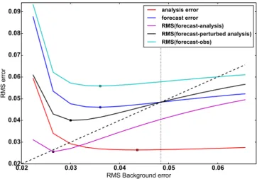
Figure 1 shows the RMS background-forecast and analysis errors as a function ofB. WhenBis small the forecast and analysis errors (dark blue line and red line, respectively) are large and the system is sub-optimal for these values. Verifica-tion against a perturbed analysis gives a systematically lower RMS error (RMSE) than verification against the truth (dark blue line) for small values of B, since insufficient weight is given to the observations. The RMS error for verification against a perturbed analysis becomes equal to that when ver-ifying against the truth for moderate values ofB(∼0.049). This point is also where the RMS error crosses the diagonal, indicating that the background errors used in the assimilation are equal to the actual background errors, and the assimila-tion is optimal. Verificaassimila-tion against observaassimila-tions gives RMS errors which are systematically higher than all the other es-timates. If observation errors are accounted for, then cation against observations becomes very similar to verifi-cation against the truth (not shown). Verifiverifi-cation against un-perturbed analyses gives smaller RMSEs than all the other methods.

The circles in Fig. 1 indicate the point at which the RMS errors are minimised for each curve. The minimum RMSE for verification against analysis (purple line) is a value ofB

around 0.026 which is much lower than the optimal value of

Bfor verification against the truth. The black line shows ver-ification against perturbed analyses and the minimum RMS error for this curve is whenB is around 0.03. This is much larger than the value of B for the minimum RMS error for verification against (unperturbed) analyses. However, this value of B, around 0.03, is much lower than the optimal (Kalman) value of around 0.049. When verifying forecasts against the truth (dark blue line) the minimum value of the forecast error is found for B around 0.036, lower than the optimal (Kalman) value. This statement may seem counter-intuitive – the lowest forecast error is found when the value of B used in the analysis is not equal to the forecast error. However, recall that the logistic map is a non-linear map and that the Kalman filter is only optimal for linear models. We have found a similar result with other models (the models of Lorenz, 1963, 1995). For both these models the forecast error is minimised when the value ofBused is larger than the ac-tual forecast error (the value given for the Kalman filter). For the logistic map the value ofBwhich minimises the analysis

0.02 0.03 0.04 0.05 0.06 RMS Background error

0.02 0.03 0.04 0.05 0.06 0.07 0.08 0.09

RMS error

analysis error forecast error RMS(forecast-analysis) RMS(forecast-perturbed analysis) RMS(forecast-obs)

Figure 1.RMS error of the forecast and analysis using the logis-tic model as a function of the background error standard devia-tion used in calculating the analysis. The red and blue lines show the RMSE for the analysis and forecast measured against the truth state. The other lines show the RMSE of the forecast, when verified against a different proxy for the truth. Verification is calculated over 200 000 analysis and forecast cycles.

error is around 0.044, closer to the Kalman value than for the forecast error – this appears to be a result consistent across the different models.

The vertical line in Fig. 1 is the point at which the cross-term< (xf−xa)T(xa−xt) >(last term of Eq. 23) is zero.

We can see that this vertical line is at approximately the same value ofB where the forecast and background errors are equal. This cross-term is plotted in Fig. 2, as the solid green line, as a function ofB. Also plotted is the correlation between the forecast and analysis errors< (xf−xt)T(xa− xt) >(blue dashed line). This is non-zero for all the values of

B run in these experiments. This demonstrates the problem in verifying against an unperturbed analysis that for all the values ofBused here the errors in the forecast are correlated with the errors in the analysis.

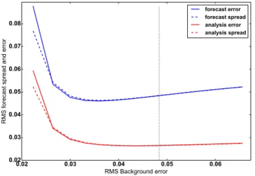
One of the conditions required for verification against per-turbed analyses to give similar results to verification against the truth is for the analysis ensemble spread to equal the RMS analysis errors (Eq. 1). The analysis and forecast ensemble spread and error is plotted in Fig. 3. The ensembles appear to be well calibrated for most values ofB. This may change if model error were introduced into the system.

6 Considering the effects of ensemble size

(6)

0.0005 0.0000 0.0005 0.0010 0.0015 0.0020 0.0025 0.0030

Cross terms

(f-t)(a-t) (f-a)(a-t)

Figure 2.Important cross-terms calculated from a long analysis cy-cle using the logistic model, as a function of the background er-ror standard deviation used in calculating the analysis. These are

< (xf−xt) (xa−xt) >(blue dashed) and< (xf−xa) (xa−xt) >

(green solid).

0.02 0.03 0.04 0.05 0.06 0.07 0.08

RMS forecast spread and error

forecast error forecast spread analysis error analysis spread

Figure 3.RMS error and ensemble spread of the forecast and anal-ysis using the logistic model, as a function of the background error standard deviation used in calculating the analysis. The ensembles were created by each ensemble member using the same assimilation method, assimilating perturbed observations.

To understand how ensemble size can affect the results, we need to return to estimates of the analysis error and spread. In Eq. (1) we relied on a cancellation of the analysis ensemble spread with the error of the ensemble mean. For a limited-size ensemble this cancellation does not hold precisely. As has been shown by Weigel (2011) the RMS error of an en-semble mean is slightly increased by effects related to the limited ensemble size. To show the limitations consider that the true state and each ensemble member are a random draw from the same distribution which has meanµand variance

σ2. We can thus write the truth as the mean of this distribu-tion plus a deviadistribu-tion from the mean

0.02 0.03 0.04 0.05 0.06 0.07 0.08 0.09

RMS error

analysis error forecast error RMS(forecast-analysis) RMS(forecast-perturbed analysis) RMS(forecast-obs)

Figure 4.RMS error of the forecast and analysis as plotted in Fig. 1, but using an ensemble with only 10 members.

xt=µ+s, (27)

where< s >=0 and< s2>=σ2. For an analysis ensemble member we would have

x_ia=µ+wi, (28)

wherewi is a random draw from the same distribution ass. Thus we may write the ensemble mean as

xa=µ+w

=µ+ 1

N

X

i=1

wi. (29)

We see thatwhas mean zero and varianceσ2/N whereNis the ensemble size. Using this Weigel (2011) showed that the mean-square error of the ensemble mean is

< xa−xt2>=< w2−2ws+s2>

=σ2 1+ 1

N

, (30)

since< w s >=0. Due to the fact that the ensemble mean is not exactly equal to the mean of the distribution, the error of the ensemble mean is slightly larger than the variance of the distribution. This is a standard mathematical result (for instance see Hoel, 1984, p. 128). Using a similar argument lets us now consider the ensemble perturbations

< x_ia−xa2>=< w_i2−2wiw+w2> . (31)

(7)

< wiw>= 1

N < w

2

i>=

σ2

N (32)

and so

< x_ia−xa2>=σ2 1− 1

N

. (33)

So, the ensemble spread is slightly smaller than the variance of the distribution due to correlations between deviations of the ensemble mean from the distribution mean and the per-turbations. This is often accounted for by using the unbiased estimator of the ensemble spread. Putting all this together, we find that for a well-calibrated ensemble

< xa−xt2>

< x_ia−xa2>

=N+1

N−1. (34)

As the ensemble size goes to infinity this ratio tends to 1 and Eq. (1) holds. However, for a limited ensemble size these differences mean that verification against analysis is not the same as verification against the truth, even when the other conditions hold. This could be corrected for if the analysis spread is known.

7 Longer lead times

As was discussed in Sect. 4 the argument that the final term in Eq. (6) is zero requires the forecast being verified to be the background for the analysis. However, we might expect that this term is zero for longer lead times, since otherwise it should be possible to produce a superior analysis. To in-vestigate this further we turn to the simple model tests used earlier.

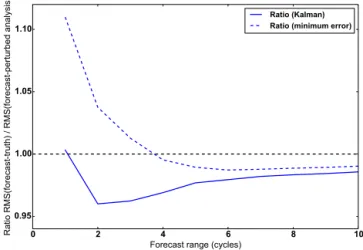
Verification for longer lead times using the system de-scribed in Sect. 5 are given in Fig. 5. This shows the ra-tio of the RMSE measured against truth to the RMSE mea-sured against perturbed analyses. This line is plotted for two choices of B. When the Kalman value of B is used the two verifications give the same RMS error at the first lead time (i.e. where the forecast is the background for the analysis). At longer lead times the RMS error when verify-ing against a perturbed analysis becomes larger than when verifying against the truth. This is caused by the final term in Eq. (6) giving a positive contribution to the verification against perturbed analysis. The interpretation is thatxt−xa

andxf−xaare positively correlated – errors in the analysis

are anti-correlated with differences between the forecast and the analysis. The correlation of analysis errors with forecast-analysis differences may be related to the use of a nonlinear model. The nonlinearity can lead to non-randomness of the errors which leads to the correlation.

Also shown in Fig. 5 is the ratio whenB is chosen to be the value which gives the minimum forecast error – for the logistic map this value is lower than the Kalman value for

0 2 4 6 8 10

Forecast range (cycles) 0.95

1.00 1.05 1.10

Ratio RMS(forecast-truth) / RMS(forecast-perturbed analysis)

Ratio (Kalman) Ratio (minimum error)

Figure 5.Ratio of the RMS errors of forecasts verified against truth and perturbed analyses using the logistic map for various lead times. For the solid line the background error was taken as the approximate Kalman value. For the dashed lineBwas taken for the value which minimises the short-period forecast error.

B. In this case verification against perturbed analysis gives smaller RMSEs than verification against the truth at short lead times. At longer lead times the verifications cross over and the RMSE against perturbed analyses is greater than the RMSE against the truth.

This behaviour at long lead times suggests that verifica-tion against a perturbed analysis is most useful at short lead times. Nonetheless it avoids the worst problems of verifi-cation against an unperturbed analysis. Therefore, we argue that it is still a useful replacement for that method of verifi-cation.

8 Verification of NWP forecasts

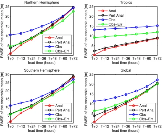
In order to understand whether this method can be applied to numerical weather prediction (NWP) systems we calculated the RMS error of a forecast ensemble mean against observa-tions and perturbed analyses. The RMS error against analy-ses was calculated at observation locations so that the quan-tities are directly comparable.

(8)

anal-T+0 T+12 T+24 T+36 T+48 T+60 T+720 5

10 15 20 25

lead time (hours)

RMSE of the ensemble mean (m)

Northern Hemisphere

Anal Pert Anal Obs Obs−Err

T+0 T+12 T+24 T+36 T+48 T+60 T+720 5

10 15 20 25

Tropics

lead time (hours)

T+0 T+12 T+24 T+36 T+48 T+60 T+720 5

10 15 20 25 30

Southern Hemisphere

lead time (hours)

T+0 T+12 T+24 T+36 T+48 T+60 T+720 5

10 15 20 25

Global

lead time (hours)

Figure 6.RMS errors of MOGREPS ensemble mean as a function of forecast lead time for forecasts of 500 hPa geopotential height. The forecast errors are reported for verification against observations and perturbed and unperturbed analyses.

yses in black, and the observations in blue, in green against the observations when the observation errors are accounted for. An observation error of 9.4 m (RMS) has been assumed. Verification against observations gives RMS errors which are systematically higher than all other estimates, while veri-fication against unperturbed analyses provides smaller RMS error than verification against observations and perturbed analyses. This is in agreement with Fig. 1. The exception is for the Southern Hemisphere, where the error against ob-servations becomes smaller than the estimates against anal-yses afterT +60 h. When observation errors are accounted for, the verification against the observations is very similar to the verification against perturbed analyses fromT+0 h to

T +36 h for the Northern and Southern hemispheres, while for longer lead times it gives lower RMS errors. This does not happen in the tropics since it is likely that verification includes the contribution of systematic errors which are not accounted for in the analysis perturbations. This is expected since 500 hPa geopotential height does not provide a good representation of what happens in the tropics.

The consistency of the RMS errors for short lead times in the northern and southern extra-tropics when calculated against perturbed analyses and observations (when subtract-ing observation error) suggests that this ensemble meets many of the required criteria. At longer lead times the RMS error against perturbed and unperturbed analyses gives larger

errors than for verification against observations, when sub-tracting observation error. This is consistent with the results in Fig. 5 – when analysis and forecast errors are no longer correlated the effect of analysis error is to over-estimate the RMSE.

9 Conclusions

We have shown that verification against a perturbed analysis gives the same RMS errors as verification against the truth, under certain conditions. These conditions require that the analysis ensemble is ideal (its RMS spread matches the RMS error in the mean analysis), that the analysis is optimal and that the ensemble size is large. Although NWP data assimi-lation systems are typically well tuned (to maximise forecast performance), none of these conditions is likely to hold ex-actly in practice. Additionally, the above results only apply to a forecast which is the background for the analysis against which it is verified.

(9)

sparsely observed, this has its own limitations. The verifi-cation results for NWP forecasts indicate it gives very simi-lar results to verification against observations, when observa-tion error is accounted for, for short lead times in the extra-tropics. Given that the problems of verification against unper-turbed analyses are most pronounced at short lead times, our method is potentially valuable for verification of short-term NWP forecasts.

It would be interesting to further explore some of the as-pects of this method. For instance, what is the effect of using an analysis ensemble which is over-spread in some areas and under-spread in others? This study also demonstrated that for a non-linear model the Kalman filter solution may not min-imise the system’s forecast error. We feel that a better under-standing of this result would be beneficial.

Acknowledgement. The analysis of limited ensemble size came about through discussion with Jonathan Flowerdew. Rob Darvell gave extensive assistance in the verification of the NWP forecasts.

Edited by: O. Talagrand

Reviewed by: five anonymous referees

References

Berre, L., Stefanescu, S., and Pereira, M.: The representation of the analysis effect in three error simulation techniques, Tellus A, 58, 196–209, 2006.

Bowler, N. E.: Explicitly accounting for observation error in cate-gorical verification of forecasts, Mon. Weather Rev., 134, 1600– 1606, 2006.

Bowler, N. E.: Accounting for the effect of observation errors on verification of MOGREPS, Meteorol. Appl., 15, 199–205, 2008. Bowler, N. E., Arribas, A., Mylne, K. R., Robertson, K. B., and Beare, S. E.: The MOGREPS short-range ensemble prediction system, Q. J. Roy. Meteorol. Soc., 134, 703–722, 2008.

Buizza, R., Houtekamer, P., Toth, Z., Pellerin, G., Wei, M., and Zhu, Y.: A comparison of the ECMWF, MSC, and NCEP global en-semble prediction systems, Mon. Weather Rev., 133, 1076–1097, 2005.

Candille, G. and Talagrand, O.: Impact of observational error on the validation of ensemble prediction systems, Q. J. Roy. Meteorol. Soc., 134, 957–971, 2008.

Ciach, G. J. and Krajewski, W. F.: On the estimation of radar rainfall error variance, Adv. Water Resour., 22, 585–595, 1999. Clayton, A. M., Lorenc, A. C., and Barker, D. M.: Operational

im-plementation of a hybrid ensemble/4D-Var global data assimila-tion system at the Met Office, Q. J. Roy. Meteorol. Soc., 139, 1445–1461, 2013.

Evensen, G.: Sequential data assimilation with a nonlinear quasi-geostrophic model using monte-carlo methods to forecast error statistics, J. Geophys. Res.-Oceans, 99, 10143–10162, 1994. Grassberger, P. and Procaccia, I.: Measuring the strangeness of

strange attractors, Physica D, 9, 189–208, 1983.

Hoel, P. G.: Introduction to mathematical statistics, 5th Edn., Wiley, 1984.

Houtekamer, P., Lefaivre, L., Derome, J., Ritchie, H., and Mitchell, H.: A system simulation approach to ensemble prediction, Mon. Weather Rev., 124, 1225–1242, 1996.

Kailath, T.: An innovations approach to least-squares estimation, Part I: linear filtering in additive white noise, IEEE T. Autom. Control, 13, 646–655, 1968.

Lorenz, E. N.: Deterministic nonperiodic flow, J. Atmos. Sci., 20, 130–148, 1963.

Lorenz, E. N.: Predictability: a problem partly solved, in: Proceed-ings of the seminar on predictability, vol. I, ECMWF, Reading, Berkshire, UK, 1–18, 1995.

Peitgen, H. O., Jurgens, H., and Saupe, D.: Chaos and Fractals: New Frontiers of Science, Springer-Velag, New York, 1992.

Saetra, O., Hersbach, H., Bidlot, J.-R., and Richardson, D. S.: Ef-fects of observation errors on the statistics for ensemble spread and reliability, Mon. Weather Rev., 132, 1487–1501, 2004. Weigel, A. P.: Ensemble forecasts, in: Forecast verification: A