A review on analytical techniques for natural convection investigation in a heated closed enclosure: Case study

A REVIEW ON ANALYTICAL TECHNIQUES FOR NATURAL

CONVECTION INVESTIGATION IN A HEATED CLOSED ENCLOSURE

Case Study

Alina Adriana MINEA

Faculty of Materials Science and Engineering, Technical University “Gheorghe Asachi”, Iasi, Romania

Review paper DOI: 10.2298/TSCI131027021M

The aim of this paper is to present a theoretical analysis of a few convection prob-lems. The investigations were started from the geometry of a classic muffle manu-factured furnace. During this analytical study, different methodologies have been carefully chosen in order to compare and evaluate the effects of applying different analytical methods of the convection heat transfer processes. In conclusion, even if there are available a lot of analytical methods, natural convection in enclosed en-closures can be studied correctly only with numerical analysis. Also, in this article is presented a case study on natural convection application in a closed heated en-closure.

Key words: heat transfer, natural convection, analytical, numerical

Importance of analytical, numerical, and experimental methods

Analytical, experimental and computational techniques are the three main approaches that may be involved for solving a problem in heat transfer [1-11].

Analysis.The equations obtained from the conservation principles to describe and pre-dict practical thermal transport processes are generally too complicated to be solved analytically and computational methods are needed to obtain the desired solution. Analytical solutions are usually obtained only for few simplified and idealized circumstances. Examples of these are transient, lumped and steady-state one-dimensional processes that lead to ordinary differential equations with constant properties that result in linear partial differential equations, and simple convective processes with a known flow field. Various analytical techniques are available for solving linear differential equations and small systems of linear equations. However, the solu-tion procedures are often quite involved and frequently lead to analytical expressions that may themselves require computation to obtain useful results [9]. Examples of these are integral trans-form methods and the method of separation of variables that are used for solving a variety of conduction problems and which lead to complicated integrals, series solutions and transcenden-tal algebraic equations which are then solved numerically. In addition, analytical techniques are usually not very versatile requiring different techniques for different boundary conditions, ge-ometries and material property variations. Analytical solutions for radiation and convective

transport can generally be obtained for extremely simplified circumstances and very few practi-cal circumstances can be considered by this approach.

Despite the limited applicability, complexity of the method and cumber-some of the analytical approach, the importance of analytical solutions can hardly be exaggerated. First, an-alytical solutions provide the means to validate the numerical model and establish the accuracy of the results. This is done by considering a relatively simple problem that is amenable to an ana-lytical solution and by comparing the results with those obtained by the numerical procedure ap-plied to the same problem [9].

Standard analytical results such as those for developed flow in a channel or pipe, con-duction in semi-infinite bodies, radiation in an enclosure with a small number of gray and dif-fuse surfaces and non-participating medium and for steady 1-D conduction in plates, cylinders and spheres are frequently used to check the accuracy and correctness of the numerical scheme. Second, analytical results, whenever available, are useful in studying the convergence, stability and other characteristics of the numerical method and for choosing the parameters which are needed for applying the scheme, such as in simulation, starting conditions for iteration and grid for discretization. Also, in the modeling and simulation of thermal systems some components may be amenable to simplification and idealization so that analysis may be used. Then, analyti-cal solutions for a few components are coupled with numerianalyti-cal solutions for the others.

The main difference between the analytical and numerical approaches is that analyti-cal methods obtain a solution that is valid everywhere in the region and at all times, within the constraints of the mathematical model, whereas numerical methods obtain results only at a finite number of discrete points and at finite time intervals. This makes it particularly attractive to use analytical methods for regions that are difficult to discretize and for short times for which nu-merical solutions may not be valid [10]. Therefore it is desirable to obtain analytical solutions whenever possible and couple these with the numerical solutions, if necessary, to cover the en-tire computational region.

Experimentation. Experiments are generally time consuming and expensive. There-fore, experimental results are usually obtained for fairly narrow ranges of operating conditions and for a selected number of configurations, dimensions and designs. However, experimental results are extremely valuable in validating the mathematical and numerical models for a given thermal process or system. Even though analytical results for simpler circumstances and the physical characteristics of the numerical results help in checking the accuracy and validity of the numerical scheme, a comparison with the experimental results from an actual system such as a prototype, are necessary to establish quantitatively the level of accuracy and confidence in the predictability of the numerical model. Though results on an actual system or process being mod-eled are desirable, costs may dictate using existing results from a similar or a simpler process. The basic approach that has been used very frequently in the simulation and design of systems is comparison between experimental and numerical results over a small region of overlap. Ones the validity and accuracy of the numerical method is established, simulation can be carried out over much wider ranges of the governing parameters in order to obtain the inputs needed for de-sign, optimization and control [10].

conjunction with the conduction problems to obtain the heat transfer coefficient. However, this is a much more complicated problem. Therefore, the use of the experimental results to obtain the value of heat transfer coefficient represents a considerable simplification in the problem. There are many other circumstances where all the information needed for the numerical model cannot be obtained by computation or analysis, and experimental inputs are needed to obtain a realistic solution. Problems involving turbulent flows, contact resistances, free surfaces, large properties changing, multiphase flows are good candidates for such experimental inputs to the numerical model [10].

Combined approaches.Analytical, experimental and computational approaches rep-resent three distinct methods to solve a given problem in heat transfer, fluid flow or energy effi-ciency. However, in actual practice, combinations of these three methods are used to obtain an approach that is best suited to a given problem [11]. As mentioned earlier, boundary conditions may be used on analysis and experimental results, and different regions may be modeled sepa-rately by different approaches. Numerical results are obtained if analytical methods cannot be used.

Similarly, experimental inputs are built into many specialized commercial software packages used to simulate certain types of systems or processes. Clearly inputs from analysis and experiments, as well as comparisons of numerical results with those from these approaches are generally desirable and necessary to obtain valid, realistic and accurate results from the nu-merical model for a given transport process or system. Comparison with analytical and experi-mental results may also be used in the developing of this solution. An example of such bench-mark solution is the computed laminar natural convection flow in a rectangular enclosure with isothermal vertical sides at a given temperature [11].

Analytical techniques in thermal transport

A consideration of the heat transfer processes is important in many industrial pro-cesses, such as welding, casting, heat treatment, in heat rejection systems; in heat removal and in problems related to our environment. As a consequence, a considerable amount of effort has been directed toward understanding the physical mechanisms that underlie processes of practi-cal interest, with a view to developing new systems and optimizing the existing ones.

Much of what is presently known about the basic characteristics of heat transfer and fluid flow processes has been obtained through analysis of the underlying physical mechanisms, by solving the governing mathematical equations, and through experimentation, carried out un-der various controlled and predetermined conditions in the laboratory. Such studies have largely focused their attention on various idealized circumstances and have employed various simplify-ing assumptions and conditions. Analytical techniques are, therefore, often very involved or in-adequate for the study of practical systems and processes. In several cases, one may resort to ex-perimentation, on a suitable simulated system in the laboratory or on the actual system itself, in order to obtain information for the prediction and optimization of the processes concerned. However, experimentation is often an expensive and time-consuming approach. As a result, whenever possible, an attempt is made to approach the problem analytically or numerically. However, available data are employed for validation of the analytical approach and for provid-ing the inputs necessary for the suitable modification and refinprovid-ing the model, in order to obtain the desired level of accuracy and predictability. Experimental methods become necessary for very complicated processes for which analytical techniques may be very difficult or inaccurate.

Also, these are very complicated and unsatisfactory for practical systems where various coupled circumstances exist. A more considerable amount of flexibility is obtained in the numerical ap-proach.

The analytical approach, though limited in its applicability, is important in evaluating the accuracy and validity of the numerical results, by considering simple problems that may be solved by available analytical techniques.

Consequently, in the next section all the general governing equations will be depicted, along with general equations for convection heat transfer. Moreover, a discussion on equations involved in convection study case is introduced. To be more specific, a discussion on free con-vection will be the focus of this article, emphasizing the free concon-vection over inclined walls and a case study is inserted in the sectionThe problem of improving energy consumptions of heating equipments.

As an outline of studied cases, a muffle furnace is considered and the improving of en-ergy consumptions is based on diminishing the heating time by heat transfer enhancement in the heated enclosure. A simple solution was adopted and at experimental and numerical level the solution gave good results [1-6]. The heat transfer enhancement was due to the presence of two inclined metallic panels that are increasing the radiation surface along with changing the con-vection flow inside the heated enclosure. The operating temperatures were about 500 °C and the focus was on how to augment the convection heat transfer by increasing the fluid velocity in the furnace chamber without external mechanical intervention. Thus, a detailed discussion on free convection will be inserted along with some details about the influence of panels presence on the heating time of the furnace.

Governing equations

The equations governing heat transfer and fluid flow processes are based on the con-servation principles for mass, momentum and energy. The concon-servation principles are very gen-eral statements that may be applied in a local sense, leading to differential equations or in a more global sense, leading to integral equations.

Mathematical background

In certain special cases the differential equations governing heat transfer and fluid flow problems involve only one independent variable and are ordinary differential equations. In some problems the dependence on two independent variables can be expressed in terms of a sin-gle variable, which is termed the similarity variable. Ordinary differential equations thus result. Though limited in application, the similarity variable method considerably simplifies a problem. The results provide a general understanding of the processes involved and form a basis for eval-uating numerical solutions of more complex equations. Local similarity and local non-similarity methods are extensions of this approach.

Partial differential equations are encountered very frequently, and numerical tech-niques for these equations have been discussed in various books [8-14]. The transient problems involve time as an independent variable and, depending on the geometry considered, one, two, or three dimensions may be needed to express the temperature distribution, the flow field, and the energy transfer rates. The simplest example of a partial differential equation involves two in-dependent variables. The form of the solution obtained either analytically or numerically, may be classified on the basis of the highest derivatives that appear in each variable.

A

x B x y C y D x E y F G

¶ ¶

¶ ¶ ¶

¶ ¶

¶ ¶

¶ ¶ 2

2

2 2

0

f f f f f

f

+ + + + + + = (1)

where the coefficients may be functions of two independent variables, represented byxandy, and of the dependent variablef(in this section,fis used to denote a general dependent variable: temperature, density, velocity, pressure). If the coefficients are independent off, being con-stants or functions ofxandy, the equation is linear inf. Both linear and non-linear equations arise in heat transfer. The mathematical character of eq. (1) is dependent on the coefficients and is said to be elliptic whenB2_{– 4AC< 0, parabolic whenB}2_{– 4AC= 0, and hyperbolic whenB}2_–

–i4AC> 0. This provides a mathematical classification, as do the boundary conditions. For ex-ample, for convection dominated flows, hyperbolic equations arise that may be solved by marching in time or along certain characteristic directions. However, non-linear partial differen-tial equations are commonly encountered in flow and heat transfer problems because of material properties that vary with the dependent variablef, radiative transport, non-linear convection terms that arise in flow momentum equations, non-linear dependence of the source onf,etc. Differential equations from heat transfer and fluid flow

The generalized form given by eq. (1) is readily simplified to obtain differential equa-tions that commonly arise in thermal-fluid problems. The simplification is achieved by specify-ing the coefficientsA,B,C, etc., as appropriate.

The Laplace and the Poisson equations, which are generally associated with steady-states problems, are commonly encountered elliptic partial differential equations and are written, respectively, as:

¶ ¶

¶ ¶ 2

2 2

2 0

f f

x y

+ = (2)

¶ ¶

¶ ¶ 2

2 2

2 0

f f

x y G

+ + = (3)

The coefficientsAandCfrom eq. (1) are equally to 1 (A=C= 1) and B is zero for these equations, resulting inB2_{– 4AC< 0. The velocity potential in invisicid, steady, incompressible}

flow satisfies the Laplace equation. The temperature distribution for steady-state, con-stant-property, 2-D conduction satisfies the Laplace equation if no thermal sources are present and the Poisson equation if a source is present.

The simplest parabolic equation in heat transfer is of the form: ¶

¶

¶ ¶

f f

y A x

= 2

2 (4)

The coefficientsBandCof eq. (1) are zero, givingB2_{– 4AC= 0 for this equation. The}

temperature in a one-dimensional transient conduction problem is governed by this equation when y and x are identified as the time and the space coordinates, respectively and A is the ther-mal diffusivity.

Hyperbolic partial differential equations (forB2_{– 4AC> 0) arise in several}

engineer-ing areas such as vibration, waves and acoustics. In heat transfer and fluid flow, hyperbolic equations describe the convection dominated flows. A simple hyperbolic equation is the first-or-der convection equation:

¶ ¶

¶ ¶ f t

f +c =

where the dependent variablef(x,t) is convected at constant velocityc. The characteristics are given by the equationx+ct= constant. Equation (5) may be differentiated with respect toxort.

Fluid flow problems generally have a non-linear term due to the inertia or acceleration component in the momentum equation. In addition, the energy equation has a corresponding term called the convection term, which involves the flow field. For transient 2-D problems, the appropriate equations are of the form:

A

x y G u x v y

¶ ¶

¶ ¶

¶ ¶

¶ ¶

¶ ¶ 2

2 2

2

f f f

t

f f

+ æ è

çç ö

ø

÷÷ + = + + (6)

wheref denotes momentum, temperature or other transported quantity, uandvare velocity components,Ais the diffusivity for momentum or heat, andG– a source term (for example due to volumetric heating in the energy equation). Equation (6) is parabolic in time (t) and elliptic in space. However, for high-speed flows, the terms on the right side dominate and the equation be-comes hyperbolic in time and space, as seen for the first-order convection eq. (5).

For radiation heat transfer problems involving a participating fluid, the source termG in eq. (6) introduces an integral over all arriving solid angles and a complicated integro-differen-tial equation results. Integral equations also appear in radiation heat transfer problems involving emitting and absorbing surfaces, with or without participating fluid. The integrals may be ap-proximated numerically, leading to algebraic equations. In the absence of participating fluid, the integral are often replaced by average values to obtain algebraic equations for the heat transfer between surfaces. Radiation problems are generally non-linear, especially when coupled with convection or conduction processes.

Boundary and initial conditions

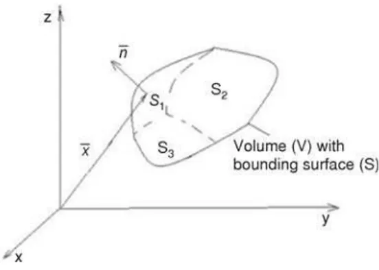
In addition to a statement of the conserva-tion equaconserva-tions, the formulaconserva-tion of a problem re-quires a complete specification of the problem geometry and appropriate boundary or initial conditions. For illustrating purposes, an arbi-trary material volume and bounding surface are sketched in fig. 1. Appropriate conservation equations are presumed to apply within the vol-ume. The number of boundary conditions re-quired is determined by the order of the highest derivatives appearing in each independent vari-able in the governing differential equations. A transient process governed by a first derivative in time will require one boundary condition (an initial condition) in order to carry out the time integration.

Spatial boundary conditions in heat transfer problems are of three general types. They may be stated in a simplified mathematical form as:

onS₁ f=f₁( )x (7)

onS

n f x

2 2

¶ ¶

f₌

( ) (8)

onS a x b x

n f x

3 ( )f ( ) 3( )

f

+ ¶ =

¶ (9)

whereS₁,S₂, andS₃denote three separate zones of the bounding surfaceSin fig. 1. The bound-ary conditions onfin eqs. (7), (8), and (9) are often referred to as Dirichlet (function), Neumann (gradient) or mixed boundary conditions, respectively. Alternatively, there are sometimes re-ferred to as being boundary conditions of types 1, 2 or 3. As stated, the boundary conditions are liner in the dependent variablef.

In heat transfer problems, Dirichlet or Neumann boundary conditions arise, respec-tively, when the temperature or the heat flux are prescribed at a boundary. Such conditions might be applied at the external boundary at a heat conducting solid or at solid walls bounding a flowing fluid. In actual practice, a constant, uniform, temperature condition at the surface arises for convective heating or cooling with a very high value of the heat transfer coefficient so that the surface temperature is essentially the fluid temperature. A constant heat flux condition is closely approximated if radiation to the surface occurs from a source which is it a much higher temperature than the surface, resulting in negligible back radiation. Mixed boundary conditions typically arise when a conducting solid is cooled by an external convective heat transfer condi-tion. For the case of fluid flow with heat transfer, the boundary conditions on the flow variables are usually expressed in terms of fluid velocities or shear stresses. Such boundary conditions are of Dirichlet or Neumann type [9, 11, 14]. When Neumann conditions are prescribed along all the bounding surfaces of a region, these conditions cannot be specified arbitrarily. For a steady-state to exist the Neumann conditions must satisfy overall heat and momentum balances in the region. In the case of radiation, the non-linear temperature dependence is generally incorporated into the functionsf₂andf₃in eq. (7) to (9).

Numerical methods for heat transfer in a closed enclosure

The two basic mechanisms by which heat is transferred are conduction and radiation. However, in many circumstances, the rate of energy transfer by these mechanisms is modified by the relative motion of the fluid that constitutes the medium in which the transport processes are occurring. This mode in which heat transfer is influenced by the fluid motion is termed con-vection. A study of convection demands consideration of the mechanisms of fluid motion in ad-dition to those related to conduction and radiation [10, 11]. Further on, consideration only on natural convection will be inserted, since are the basis of this research on saving energy in heat-ing equipments.

Numerical methods for convection heat transfer

Growing interest and research activity in convective transport have been seen in recent years because of its relevance to a wide range of important problems. The need to optimize in-dustrial processes, particularly with respect to energy, has led to a study of convective processes that are crucial in determining the energy requirements and the quality of the product. The de-sign and operation of the furnaces, ovens, power plants, automobiles, airplanes and other sys-tems require detailed information on the relevant convective processes [10].

The basic equations that govern convective processes are obtained from the conservations laws for mass, momentum and energy. Considering a given location for the flow, ifris the density of the fluid andVthe local velocity, the conservation of mass gives [10]:

¶ ¶ r

t r

+ Ñ( )=

r

V 0 (10)

Therefore, for steady flow, eq. (10) is known as the continuity equation and is written as:

Ñ(r )=

r

V 0 (11)

and if the density is constant:

Ñ =r

V 0 (12)

In the Cartesian co-ordinates: ¶ ¶ ¶ ¶ ¶ ¶ u x v y w z

+ + =0 (13)

whereu,v,ware the velocity components in x, y, z directions, respectively.

The principle of conservation of momentum, which equates the rate of change of mo-mentum to the forces applied, gives themomentum equation(or theequation of motion). The time rate of increase of momentum of a fluid within a fixed control volume will be equal to the rate at which momentum flows into the domain through its confining surfaceS, plus the net force acting on the fluid within the considered domain. When the flow is incompressible, the viscosity is constant, and the flow is laminar, the Navier-Stokes equations result. In Cartesian co-ordinates, withF_x,F_y, andF_ztaken as the components of the body force per unit volume, the Navier-Stokes equations are [10]:

r t m ¶ ¶ ¶ ¶ ¶ ¶ ¶ ¶ ¶ ¶ ¶ ¶ ¶ ¶ u u u x v u y w w z p x u x u + + + æ è çç ö ø

÷÷ = - + 2 +

2 2 y u z F 2 2 2 + æ è çç ö ø ÷÷ + ¶

¶ x (14)

r t m ¶ ¶ ¶ ¶ ¶ ¶ ¶ ¶ ¶ ¶ ¶ ¶ ¶ ¶ v u v x v v y w w z p y v x v + + + æ è çç ö ø

÷÷ = - + 2 +

2 2 y v z F 2 2 2 + æ è çç ö ø ÷÷ + ¶

¶ y (15)

r t m ¶ ¶ ¶ ¶ ¶ ¶ ¶ ¶ ¶ ¶ ¶ ¶ ¶ ¶ w u w x v w y w w z p z w x w + + + æ è çç ö ø

÷÷ = - + 2 +

2 2 y w z F 2 2 2 + æ è çç ö ø ÷÷ + ¶

¶ z (16)

The energy equation is obtained from the principle of conservation of energy, as ap-plied to a differential fluid element. The commonly used form of the energy equation is:

r

t r t b t m

C DT

D C

T

V T k T q T Dp

D

p = p + Ñ

é ëê

ù

ûú= Ñ + + +

¶ ¶

D

( ) ( ) _v F (17)

In this equation,¶T/¶trepresents the transient effects, (VÑ) the convective part of the heat transfer,Ñ(kÑ_{T) the conductive part,q}

vthe thermal sources per unit volume and time,

bT(Dp/Dt) the pressure work, and mfthe viscous dissipation effect, representing the irrevers-ible part of the energy transfer due to viscous forces. The parameterbis the coefficient of ther-mal expansion of the fluid and is given by:

b r

r = - æ

è ç ö ø ÷ 1 ¶ ¶_T p (18)

If it simplifies eq. (17) for Newtonian fluids having constant density and viscosity and in absence of volumetric heat sources it obtain:

r t

C T u T

x v T

y T

z k

T x

T y

p

¶ ¶

¶ ¶

¶ ¶

¶ ¶

¶ ¶

¶ ¶

¶

+ + +

æ è

çç ö

ø

÷÷ = 2 + +

2 2

2 2_T

z ¶ 2

æ è

çç ö

ø

÷÷ (19)

In natural or free convection flows the basic mechanism generating the flow is the buoyancy force which arises due to temperature differences in the fluid. The body forceFis non-zero and is replaced by rg, where g is the gravitational acceleration for flow in a gravita-tional force field. The density difference gives rise to a buoyancy force which appears in the mo-mentum equation and generates the flow. Therefore, the momo-mentum and the energy equations are inevitably coupled for free convection flows. This generally makes the solution of free con-vection problems much more difficult, as corresponding constant property forced convective circumstances. Many important approximations are, therefore, often made in free convection to make the problem well brought-up [10].

As a partial conclusion, the real mathematical model that describes the air circulation in electric furnaces (free convection dominant) can be described by eqs. (11), (14), (15), (16), and (17). Moreover, one can add the radiation heat transfer. As an observation, these equations cannot be solved for the general case, and needs assumptions and simplifications together with specific boundary conditions. Further on, some considerations about the possibilities to obtain a realistic solution are given.

Empirical approach for convection heat transfer

In several problems of practical interest, the heat transfer and flow processes are so complicated that the analytical and numerical methods discussed earlier cannot be employed easily and one has to depend on experimental data [8-10]. Over the years, a considerable amount of information on heat transfer rates for various flow configurations and thermal conditions has been gathered. Some of this information has already been presented earlier. The present section gives some of the commonly used results for a few important cases. The results included here are only a small fraction of what is available in the literature, and the attempt is only to present use-ful results in a few common circumstances and to indicate the general features of the empirical relationships. Unless mentioned otherwise, all fluid properties are to be evaluated at the film temperatureT_f= (T_w+T₄)/2.

Increasing the convection heat transfer rate is accomplished by increasing the fluid ve-locity. The empirical method to study convection in furnaces is based on Nusselt number, Reynolds number, Grashof number, and Prandtl number [8-15]. This method is widely used in furnace operation practice and recommended by Trinks in its works [8].

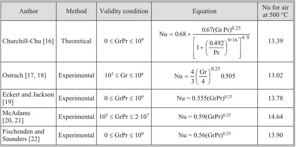
There are a lot of approaches in this area, almost all based on experimental observa-tions. Some of them are outlined in tab. 1 together with the results obtained from simulation for the case of rectangular furnace with no panels inside [1-6]. As one can notice from tab. 1, similar results are obtained from all equations. The results were calculated for heating up to 500 °C con-sidering air as an ideal gas and all the properties at 500 °C. Therefore, it obtains Pr = 0.686 and Gr = 0.56·10–6_{, resulting a laminar flow (10}4_{< GrPr < 10}8_).

For forced convection it can apply [8]:

Nu=hL=

k C

x y

The Nusselt number, Nu, is a dimensionless number whereinC,x, andyare constants determined by experiment or experience for specific fluids, configurations, and temperatures. Values for all fluid properties, including Prandtl number, Pr, should be evaluated at an estimated mean film temperature-mean between bulk stream temperature and wall surface temperature. The Nusselt number, is a dimensionless ratio of convection to conduction capabilities of the fluid, whereinhis the convection film coefficient, andL– the length of the surface parallel to the gas flow if less than 0.61 m [8].kis the thermal conductivity of the gas.

Re= r m

vL

(21) The Reynolds number, Re, is a dimensionless ratio of momentum to viscous forces in the heat-ing or coolheat-ing fluid, whereinrV= momentum, in whichris the density andv– the velocity, and m– the absolute viscosity, all at mean film temperature.

Pr=c k

pm

(22) The Prandtl number, Pr, is a dimensionless ratio of fluid properties that affect heat flow, whereinc_pis the specific heat,m– the absolute or dynamic viscosity, andk– the thermal conductivity. Values of the Prandtl number range from 0.65 to 0.73 for most gas mixtures and is about 0.65 for air [8].

Gr=L g T

2

2

b n

D

(23) The Grashof number, Gr, is a dimensionless number in fluid dynamics and heat trans-fer which approximates the ratio of the buoyancy to viscous force acting on a fluid. It frequently arises in the study of situations involving natural convection, whereinLis the flow length, g – the acceleration due to Earth's gravity;b– the volumetric thermal expansion coefficient (equal to approximately 1/T, for ideal fluids, whereTis the absolute temperature),D_T

s– the

tempera-ture difference,n– the kinematic viscosity.

Table 1. Empirical correlations for describing air natural convection in laminar flow, applied to enclosures and plates

Author Method Validity condition Equation Nu for air

at 500 °C

Churchill-Chu [16] Theoretical 0£GrPr£109

Nu= + Gr

+æ è

ç ö

ø ÷ é

ë ê ê

ù

û ú ú

0 68 0 67

1 0 492

0 25

9 16 4

. . ( Pr)

. Pr

.

/ / 9 _13.39

Ostrach [17, 18] Experimental 103_£Gr£106 _Nu= æGr

è ç ö

ø ÷

4

3 4 0 505

0 25.

. 13.02

Eckert and Jackson

[19] Experimental 0£GrPr£10

9 _{Nu = 0.555(GrPr)}0.25 _13.78

McAdams

[20, 21] Experimental 10

5_{£GrPr£2·10}7 _{Nu = 0.59(GrPr)}0.25 _14.64

Fischenden and

Saunders [22] Experimental 0£GrPr£10

Jaluria [23] is offering some useful information on natural convection in enclosures, based on Nusselt and Raylingh numbers calculated on the distancedbetween heated walls. In the mentioned book, one can find the Catton correlation:

Nu=

+ æ è

ç ö

ø ÷ 018

02

0 29

. Pr

. Pr

.

(24)

As a conclusion, there are no correlations in the literature to link the air rate (through Reynolds number) and surface heat transfer coefficient (calculated from the Nusselt number), mainly because the natural convection is a buoyancy driven process and the air rate is not mea-surable and is not an independent variable. In these conditions, one has to apply a different ap-proach.

Dimensionless analysis

Another approach, more accurate, can be the numerical one starting from the convec-tion basic equaconvec-tions presented earlier and considering the general case of natural convecconvec-tion on a vertical surface in laminar flow. The general case of natural convection over inclined surfaces is a theory based case and it is presented in almost all Heat Transfer books [8-24]. The system of differential equations to be solved is obtained in 2-D flow considering the Boussinesq aproximation [8]:

¶ ¶

¶ ¶ ¶

¶ ¶ ¶

¶ ¶ ¶

¶ ¶ ¶ u x

v y

u u x v

v

y g T T v

v y

u T x v

T y

f

+ =

+ =

-+ =

0

2

2

b ( )

a T

y ¶ ¶ 2

2 (25)

and is subject to boundary conditions: BC1:y= 0,u= 0,v= 0,T=T_w, and BC2:y=4,u= 0, ¶v/¶y= 0,T=T₄.

Even in the simplified boundary layer form derived, the equations have not been solved in closed form. Instead, numerical results have been obtained, known as the Ostrach so-lution (see Convection Heat Transfer, ch. 7 [10]). The Ostrach soso-lutions are presented graphi-cally as dependence between Prandtl number and Grashof number. In using this evaluation, the fluid temperature is evaluated at the medium film temperature.

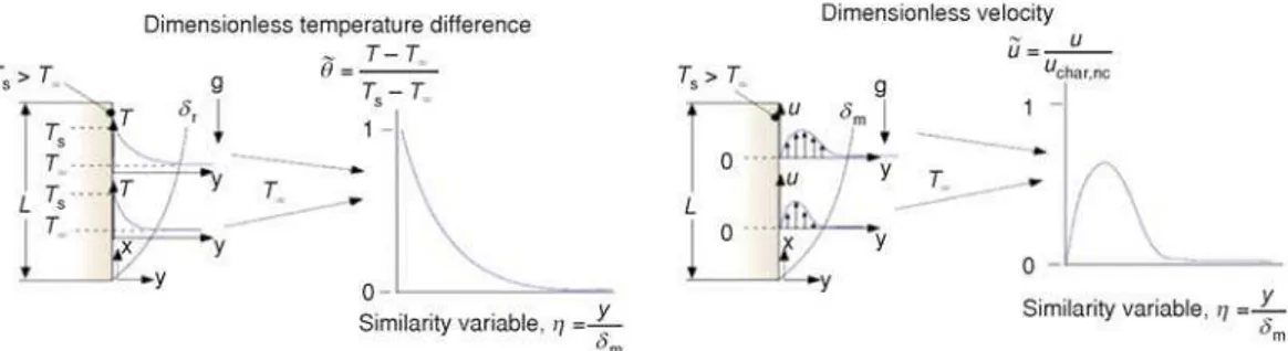
Figure 2 illustrates, qualitatively, the velocity and temperature distributions that are expected adjacent to a vertical, isothermal, heated flat plate under laminar conditions. The simi-larity solution is based on the idea that the temperature and velocity distributions at any position

along the plate surface,x, will collapse if they are plotted in dimensionless form as a function of an appropriately defined similarity variable. This method is called "Similarity solution for natu-ral convection" and requires computational effort [10-13].

However, there are many natural convection flows that occur within enclosed regions, such as flows in rooms and buildings, cooling towers and furnaces. The flow domain may be completely enclosed by solid boundaries or may be a partial enclosure with openings through which exchange with the ambient occurs. There has been growing interest and research activity in buoyancy-induced flows arising in partial or complete enclosures. Much of this interest has arisen because of applications such as cooling of electronic circuitry, building fires, materials processing, and environmental processes [9]. The basic mechanisms and heat transfer results in internal natural convection have been reviewed by several researchers, such as Ostrach [18]. Some of the important basic considerations are presented here.

The 2-D natural convection flow in a rectangular enclosure, with the two vertical walls at a constant heat flux or temperature and the horizontal boundaries taken as adiabatic or at a temperature varying linearly between those of the vertical boundaries, has been thoroughly in-vestigated over the past three decades. The resulting boundary layer equations for a 2-D vertical flow, with variable fluid properties except density, for which the Boussinesq approximations are used, are written as [23]:

¶ ¶ ¶ ¶ ¶ ¶ ¶ ¶ ¶ ¶ ¶ ¶ u x v y u u x v v

y g T T y

u y

f

+ =

+ = - + æ

è çç ö ø ÷÷ 0 1 b r m ( )

rc u T b

x v T

y y k

T

y q Tu

p

p v a

¶ ¶ ¶ ¶ ¶ ¶ ¶ ¶ ¶ ¶ + æ è çç ö ø ÷÷ = æ

è çç ö ø ÷÷ + + x u y + æ è çç ö ø ÷÷ m ¶ ¶ 2 (26)

wherep_ais due to the hydrostatic pressure and the last two terms in the energy equation are the dominant terms from pressure work and viscous dissipation effects. Hereuandvare the velocity components in the x- and y-directions, respectively. Although these equations are written for a vertical, two-dimensional flow, similar approximations can be employed for many other flow circumstances, such as axisymmetric flow over a vertical cylinder and the wake above a concen-trated heat source.

There are several other approximations that are commonly employed in the analysis of natural convection flows. The fluid properties, except density, for which the Boussinesq ap-proximations are generally employed, are often taken as constant. The viscous dissipation and pressure work terms are generally small and can be neglected. So eq. (26) for no heat generation (q_v= 0)[23]:

¶ ¶ ¶ ¶ ¶ ¶ ¶ ¶ ¶ ¶ ¶ ¶ u x v y u u x v u

y g T T y

u y

+ =

+ = - + æ

è çç ö ø ÷÷ 0 1 b r m

( _f)

rc u T x v

T

y y k

T y p ¶ ¶ ¶ ¶ ¶ ¶ ¶ ¶ + æ è çç ö ø ÷÷ = æ

è çç ö

ø ÷÷

(27)

u

y v x

v x u x =¶ = - = -¶ ¶ ¶ ¶ ¶ ¶ ¶ Y Y

, , w (28)

are, in dimensionless form [10, 23, 24]: ¶ ¶ ¶ ¶ ¶ ¶ ¶ ¶ ¶ ¶ ¶ ¶ ¶ ¶

(U ) ( )

X

V

Y X Y y

X Y

W W W W

Y Y + = + -+ = 2 2 2 2 2 2 2 2 Gr q

-+ = æ +

è ç ö ø ÷ W ¶ ¶ ¶ ¶ ¶ ¶ ¶ ¶ ( ) ( ) Pr U X V

Y X Y

q q 1 q q

2 2 (29)

where the dissipative term and that involving the material derivative of the pressure were ne-glected.

Equation (29) were derived under the hypotheses of laminar, 2-D flow, steady-state re-gime and taking the thermo-physical properties to be constant with temperature except for the density, as suggested by the Boussinesq approximation. The employed dimensionless variables for a rectangular enclosure are [10]:

X x b Y y b U ub V vb

P p p b T T k

qb = = = = = - = - = , , , ( ) , ( ) , n n rn q y 4 4 2

2 Y _n

w n b n n ,

, Pr , Pr

W= = = = b qb k a 2 4 2

Gr g Ra Gr (30)

wherebis the enclosure width. In eqs. (28), (29), and (30) the notations are: g is the acceleration due to the gravity; Pr – Prandtl number;u,v– the velocity components along x, y;U,V– the dimensionless velocity components; x, y – the Cartesian co-ordinates;X,Y– the dimensionless coordinates;q– the dimensionless temperature;y– the stream function;Y– the dimensionless stream function;w– the vorticity;W – the dimensionless vorticity;p– the pressure;P– the dimensionless pressure;n– kinematic viscosity.

Equations (29) can be solved by imposing the boundary conditions. Andreozzi in her work [25] on a symmetrical heated enclosure considered the following assumptions: a uniform heat flux and no-slip condition on the channel plates; adiabatic wall and no-slip condition on the other solid walls; boundary at ambient temperature and normal component of the velocity gradi-ent equal to zero on the enclosure and adiabatic boundary.

A parametric analysis of a chimney-type enclosure was carried out by Andreozzi [25] and the results were delivered for air, Pr = 0.71, for different enclosure aspect ratio. No local flow separation around the entrance corner was found in all considered cases. In the following, correlations of the dimensionless flow rate (equal to Reynolds number) and the average Nusselt number as a function of the channel Rayleigh number are reported from Andreozzi [25]. In par-ticular, for the flow rate, the following equation is proposed:

D_Y= æ

è ç ö ø ÷ æ è ç ö ø ÷ æ -3 590 0 2323

0 7323 0 2677

, . . . Ra h h L b B b L L è çç ö ø ÷÷

0 4823.

(31)

For the average Nusselt number, the following equation was proposed:

Nu Ra

h

=æ è ç ö

ø

÷ æ

è çç ö

ø

÷÷ æ_èç ö ø ÷

-B b

L L

B b

0 250 0 150 0

0570

. . .

.

360 11 0 161 11

1155 é

ë ê ê

ù

û ú ú

+ æ

è

ç ö

ø ÷ é

ë ê ê

ù

û ú ú ì

í ï

î

-

-.

.

RaB b ï

ü ý ï

þï -1 11/

(32)

As one can notice from eqs. (31) and (32), the heat transfer coefficient enhancement is directly influenced by the increasing of the Rayleigh number, thus by increasing the stream function (expressed by the Reynolds number and fluid velocity in dimensionless variables).

The problem of improving energy consumptions of heating equipments

Batch ovens and low-temperature batch furnaces (200-760 °C) are in a range where convection capability may exceed radiation capability. Convection is used for effective heating in this temperature range where radiation is weak or has a “shadow problem” because it travels only in straight lines. Increasing the convection heat transfer rate is generally accomplished by using circulating fans, by using high-velocity burners, by judicious load placement and spacing, and by enhanced heating. In this article, a new method for enhancing convection is proposed, by placing inclined panels in the enclosure. The convection enhancement leads to diminishing the heating time and thus to decrease the energy consumption for heating [8].

Mathematical model for heat transfer enhancement in studied heating equipment

Studied heating equipment is a batch furnaces of low volume that is working at me-dium temperatures. The studied heating cycle is up to 500 °C. In this temperature range, convec-tion capability is exceeding radiaconvec-tion. The aim of this case study is to save energy by reducing heating time and this goal can be achieved by augmenting heat transfer in the heated enclosure. All the experiments and the CFD analysis presented in previous works [1-7] are sustaining the idea of introducing two inclined radiant panels in the fur-nace chamber, as shown in fig. 3. The physical explana-tion is that the presence of the panels is of benefit for the total heat transfer coefficient.

The two involved mechanisms for heating in the considered enclosures are radiation and free convection. Radiation is simply enhanced by enlarging the heat trans-fer surface, thus the heat transtrans-ferred by radiation is in-creasing. Convection heat transfer is strongly influenced by the panels position that determines the air rate between the walls and the panels.

A useful approach of this method is the dimensionless analysis explained before. Further on it will keep in mind eqs. (31) and (32) derived by Andreozzi [25] with the help of dimensionless analysis and the associated parametric study. These equations were determined for chimney-type channels in internal natural convection flows for rectangular enclosures. And this analysis can be successfully applied to heating equipments with panels in-side. Each panel is forming a chimney-type channel be-Figure 3. Sketch of the studied

tween the heating region and the panel itself, creating two chimney-type channels in the enclo-sure. These channels are directing the flow and are modifying the natural convection.

For a specific case of a furnace with dimensions depicted in [5], it can consider the Andreozzi [24] dimensions factors as:B/b= 1,L/L_h= 1, andL_h/b= 1 and equations are:

D_{Y= 3.590Ra}0.2323 ₍₃₃₎

Nu=[ .₀₅₇₀(Ra)0 306. ]-11 +[ .₁₁₅₅(Ra)0 161. ]-11}-1 11/ ₍₃₄₎

If it combines these equations in term of the Rayleigh number, one can obtain: Nu=[ .₀₁₀₅₈(D_Y)1 3173. ]-11 +[ ._{0 4763}(D_Y)0 6931. ]-11}-1/11 ₍₃₅₎

and if it applies the Nusselt number correlation, one can get for panels of heightL: h=k

L[ . ( ) ] [ . ( ) ] }

. .

01058D_Y 1 3173 -11 + 0 4763 D_Y 0 6931 -11 -1/11 ₍₃₆₎

or for inclined panels at an anglea:

h k

L

= - +

-cos {[ . ( ) ] [ . ( ) ]

. .

a 01058 0 4763

1 3173 11 0 6931

D_Y D_Y 11_}-1 11/ ₍₃₇₎

As a conclusion, eq. (37) can be used to model the heat transfer coefficient based on panel length and inclination, thermal conductivity of the heating fluid and the associated stream function. This equation was considered as a base for energy saving possibilities in an electrical furnace with natural convection. Later on, the experimental and numerical tests will consider in-creasing air velocity as a base for enhancement of natural convection that can lead to augment the overall heat transfer in the enclosure and decreasing of the heating time. Thus, this technique will go on minimizing the energy consumption for heating "thin parts" in the furnace.

Modeling possibilities for saving energy in heating equipments

Considering a heating process in a furnace with a temperatureT_fover a wide tempera-ture range, the load starting at a temperatempera-ture of T_w1and ending atT_w2, a medium load tempera-tureT_mcan be assumed, for which a medium heat transfer coefficient can be determined. The heating timetmay be calculated as:

q=Q/A – heat conveyed to the square meter surfaceA[m²] of the load, ¶Q=hA(T_f–T_w)¶t – heat supplied to the surface of the load during time, and

¶Q=mc_p¶T_w – heat leading to a change in temperature of a load of mass m and heat

– capacityc_p[Jkg–1_K–1_]

hA T( _f -T_w)¶_t=V c_{r p}¶T_{w (38)} hA

c V

T

T T

p

r t

¶ = ¶

-w

f w

(39) whereas

A V

A As s A

V

r L

r L r ...

= =

= =

1

2 2

2

...for the plate

for the p

p cylinder

for the sphere A

V R

R R ...

= 4 =

4 3

3

2 3 p p

The parametersis for a single sided heated plate the thickness of the plate, respec-tively, half the thickness for a double sided heated plate.

h T T sc T h

c s T T T

p

p

( _{f w}) _w

f w w

- Þ

-¶_{t = r} ¶ ¶ = ¶

r t

1

(41)

After integration and applying boundary conditions:

t t t t t

r = ₁ =0; C=ln(T -T ₁); = ₂ =0; C=ln(T -T )+ h

c_p s

f w f w2

the heating timetcan be estimated with:

t= - r

-c s h T T T T p

ln f w

f w 2

1

(42)

Moreover, saving energy possibilities for heating thin loads may rely on combining eq. (36) with eq. (42):

t= - r

+ -c s k L p

{[ .₀₁₀₅₈(D_Y)1 3173. ] 11 [ ._{0 4763}(D_Y)0 6931. ]-

-11 1 11

2 } ln / T T T T f w f w1 (43)

wherec_p,r, andsare the specific heat, density, and dimension of the load,L– the panel length (or the wall length for furnaces without panels), D_{Y – the stream function (similar to the} Reynolds number, depicting the air rate) inside the heated chamber, andk– the conductivity of the air at operating temperature (T_f).

Or, if it considers the furnace with inclined panels at an angle, aone can get:

t r a = -+ -c s k L p

cos {[ . ( ) ] [ . ( )

. .

01058D_Y 1 3173 11 0 4763D_Y 0 6931 11 1 11

2 ] } ln / - -T T T T f w f w1 (44)

If it goes further and consider a furnace with known maximum power supply,P, work-ing for a specific time,t, the consumed energy can be written as:

E

Y Y

= =

+

-P P c s

k L

p

t r

{[ .₀₁₀₅₈(D )1 3173. ] 11 [ ._{0 4763}(D )0 69. 31 11 1 11

2 ] } ln / - -T T T T f w f w1 (45)

and for inclined panels: E

Y Y

=

+

-P c s

k L

pr

a

cos {[ . ( ) ] [ . ( )

. .

01058D 1 3173 11 0 4763 D 0 6931 11 1 11

2 ] } ln / - -T T T T f w f w1 (46)

From eqs. (43) and (45) one can notice the influence of the heating time and stream function, respectively, on the energy consumption of a certain furnace working at maximum heating power. This equation is the base for optimization of furnace heating for “thin loads” where no special prescriptions are needed for heating. The saving energy technique applied and described in this paper considered different types of panels (thick, thin, standard, and perfo-rated) under different inclinations,a. The chimney type effect on air rate in natural convection was studied and final energy consumption was monitored through total heating time, as ex-pressed in eq. (46).

describes the possibilities of saving energy by decreasing the heating time for “thin loads” and increasing the air rate inside the furnace chamber, thus by intensifying convection and convec-tion coefficient, respectively. Parameters considered as variables for the experimental and nu-merical study are the panels position, surface and thickness that can lead to increasing the air ve-locity by creating the chimney effect with a result in augmenting natural convection. This equation is based on the dimensionless approach for natural convection heat transfer in chim-neys type enclosures.

Conclusions

Convection heat transfer is a very complicated mechanism that can be described with a system of at least 4-5 differential equations with difficult boundary layer approximations. More-over, all the fluid properties are variable with temperature and, thus, the equations became more complicated. Off course, in almost all analytical studies, the thermo-physical properties can be considered constant on little to no temperature variation. Anyway, for natural convection, the fluid density is mandatory considered as variable. In this particular case, as was affirmed before, it is very hard to employ an analytical approach and the obtained system of differential equations needs to be solved by a numerical approach with the help of the computer. Far as the author knows, there are no such analytical approaches in the literature. The pure analytical approaches considered in the published researches (available in Science Direct, Web of Science or special-ized books) are based on a lot of simplification hypothesis that are very hard to meet in practice and on very simple configurations (like tubes or plates). In the case of furnaces heat transfer studies, the most common approach is experimental and later on the CFD simulation.

Considering the present situation, of an electric furnace heated at 500 °C that works mostly on natural convection, the numerical approach is the only theoretical approach that is available; otherwise the mathematical system of equations cannot be handled in simplifications that do not alter the physical processes. The possibility of the physical processes alteration exists in any simulation, so author believe that an experimental validation is mandatory, when is avail-able. On another hand, any experiment can be amended by errors generated by the instrumenta-tion, thermocouples precision or posiinstrumenta-tion, initial or final conditions. So, when is possible, a nu-merical analysis is welcomed.

Anyway, as a basic analytical approach, the use of the similarity variable method was chosen to physically connect the convection heat transfer coefficient with the air rate variation in the enclosure. As one can see in numerical methods for heat transfer in a closed enclosure it is almost impossible to get a correct dependency between the convection heat transfer coefficient and the fluid air rate in natural convection. In forced convection, such a correlation is easy to ob-tain since the Nusselt number depends on the Reynolds number and the fluid rate is an independ-ent variable. On the other hand, in natural convection, the Reynolds number does not interfere and the Nusselt number is dependent on the Prandtl number and the Grashof number, and this is because fluid rate is a dependent variable (natural convection is buoyancy driven process). In this situation, author used the similarity variable method and the streamline function that de-scribe very well the fluid rate in the enclosure. Also, for the specific case of panels insertion, the chimney effect was adopted.

be-tween different heating regimes was detailed in [1-6] and variation of heating time was noticed by introducing the panels and results were in agreement with eq. (44). The explanation was that by introducing the panels, the air rate in the boundary layer,v, was increased and a decreasing of heating time,t, was noticed. If it refers to eq. (46), the energy consumption by heating at maxi-mum power is decreasing while the heating time is decreasing and air rate increasing.

As a final conclusion, a possibility of saving energy in studied furnaces was identified as enhancing convection heat transfer by changing the air rate profile and intensifying air circu-lation in the enclosure by a simple method of introducing metallic panels and creating the chim-ney effect. This technique was validated both by experimental tests and CFD simulations as out-lined in [1-6].

References

[1] Minea, A. A., An Experimental Method to Decrease Heating Time in a Commercial Furnace, Experimen-tal Heat Transfer, 23(2010), 3, pp. 175-184

[2] Minea, A. A., Dima, A., Saving Energy through Improving Convection in a Muffle Furnace,Thermal Sci-ence Journal, 12(2008), 3, pp. 121-125

[3] Minea, A. A., Experimental and Numerical Analysis of Heat Transfer in a Closed Enclosure,Metalurgija, 51(2012), 2, pp. 199-202

[4] Minea, A. A, Simulation of Heat Transfer Processes in an Unconventional Furnace,Journal of Engineer-ing Thermophysics, 19(2010), 4, pp. 31-38

[5] Minea, A. A., Experimental and Empirical Technique to Estimate Energy Decreasing at Heating in an Oval Furnace,Metalurgija, 51(2012), 4, pp. 473-476

[6] Minea, A. A., A Comparison Study on Experimental Heat Transfer Enhancement on Different Furnaces Enclosures,Heat and Mass Transfer, 48(2012), 11, pp. 1837-1845

[7] Minea, A. A., Advances in Industrial Heat Transfer, CRC Press Taylor & Francis, Boca Raton, Fla., USA, 2012

[8] Trinks, W.,et al.,Industrial Furnaces, 6th_{ed., John Wiley and Sons, New York, USA, 2004}

[9] Pop, I., Ingham, D. B., Convective Heat Transfer: Mathematical and Computational Modelling of Viscous Fluids and Porous Media, Elsevier, USA, 2001

[10] Bejan, A, Krauss, A,Heat Transfer Handbook, John Willey and Sons, New York, USA 2003 [11] Janna, W. S.,Engineering Heat Transfer– 2nd_{ed., CRC Press, Boca Raton, Fla., USA, 2001}

Nomenclature

c_p – specific heat, [Jkg–1_K–1_]

g – acceleration due to Earth's gravity,

– [ms–1_]

Gr – Grashof number, [–]

k – thermal conductivity, [Wm–1_K–1_] L – is the flow length, [m]

Nu – Nusselt number, [–]

P – dimensionless pressure, [–]

p – pressure, [Nm–2_]

p_a – is due to the hydrostatic pressure,

– [Nm–2_]

Pr – Prandtl number, [–]

q_v – the thermal sources per unit volume

– and time, [Wm–3_]

Ra – Rayleigh number, [–]

S1, S2 S3– denote three separate zones of the

– bounding surfaceS, [m2_]

T – temperature, [K]

U,V – dimensionless velocity components, [–]

u, v, w – are the velocity components in x, y, z

– directions, [ms–1_]

X, Y – dimensionless coordinates, [–]

x, y – Cartesian co-ordinates, [m]

Greek symbols

b – volumetric thermal expansion

– coefficient, [K–1_]

q – dimensionless temperature, [–] m – absolute viscosity, [kgm–1_s–1_]

n – kinematic viscosity, [m2_s–1_]

r – density, [kgm–3_]

f – denote a general dependent variable:

– temperature, density, velocity, pressure Y – dimensionless stream function, [–] y – stream function, [m2_s–1_]

[12] Sahoo, P.K.,et al., A Computer Based Iterative Solution for Accurate Estimation of Heat Transfer Coeffi-cients in a Helical Tube Heat Exchanger,J. Food Eng. 58(2003), pp. 211-214

[13] Karlekar, B.V., Desmond, R. M.,Heat Transfer, West Publishing Co., St. Paul, Minn.USA, l982 [14] White, F. M.,Heat Transfer, Addison-Wesley Publishing Company Inc., New York, USA, 1984 [15] Minea, A. A., Dima, A., CFD Simulation in an Oval Furnace with Variable Radiation Panels,Metalurgia

International, XIII (2008), 10, pp. 9-14

[16] Incropera, F. P., DeWitt, D. P.,Fundamentals of Heat and Mass Transfer(4th_{ed.), John Wiley and Sons,}

New York, USA, 2000

[17] Ostrach, S., Natural Convection in Enclosures, in:Advances in Heat Transfer(Ed. J. P. Hartnett, T. F. Ervine),Vol. 8, Academic Press, New York, USA, 1972, pp. 161-227

[18] Ostrach, S., Natural Convection in Enclosures,J. Heat Transfer , 110(1988), 48, pp. 1175-1190 [19] Eckert, E. R. G., Jackson, T. W., Analysis of Turbulent Free-Convection Boundary Layer on a Flat Plate,

NACA TR 1015, 1951

[20] Welty, J. R.,et al., Fundamentals of Momentum, Heat and Mass transfer (5th_{ed.). John Wiley and Sons,}

New York, USA, 2007

[21] McAdams, W. H., Heat Transmission, 3rd ed., McGraw-Hill, New York, USA, 1954

[22] Fischenden, M., Saunders, O. A., The Calculation of Heat Transmission, His Majesty's Stationary Office, London, 1932

[23] Jaluria, Y., Natural Convection Heat and Mass Transfer, Pergamon Press, Oxford, UK, 1980

[24] Jaluria, Y., Torrance, K. E., Computational heat transfer, 2nd_{ed., Taylor and Francis, New York, USA,}

2003

[25] Andreozzi, A.,et al., Thermal Management of a Symmetrically Heated Channel-Chimney System, Inter-national Journal of Thermal Sciences, 48(2009), pp. 475-487