NEW TRENDS IN MATHEMATICAL SCIENCES
Vol. 2, No. 3, 2014, p.178-189ISSN 2147-5520 - www.ntmsci.com
Analytical investigation for fluid behavior over a flat plate with
oscillating motion and wall transpiration
F.Farkhadnia
a, R.Kamrani
a, D. D. Ganji
b,1aDepartment of Mechanical Engineering, Mazandaran Institute of Technology, Babol, Iran b
Babol University of Technology, Department of Mechanical Engineering, Babol, Iran
Abstract: In this paper, fluid behavior over a flat plate with oscillating motion, starting from rest and wall transpiration is presented. The classical solution of this problem is given by Panton [22] and is found to be an especial case of the solution here presented. The analytical solution is obtained without the use of any special transformations, such as Laplace or Fourier transforms. Three highly accurate and simple semi analytical methods, Variational Iteration Method (VIM), Homotopy Perturbation Method (HPM) and Adomians Decomposition Method (ADM) are used to solve this problem. The results show the effects of suction and injection of the wall on fluid behavior and reveal that VIM, HPM and ADM are very effective and accurate in comparison with the exact solution. A non-dimensional number is used to take in to account the injection or suction of fluid at the wall. This parameter is shown to be of great influence on the proposed velocity solution.
Keywords: Semi Analytical Methods (ADM, HPM, VIM); Oscillating wall; Navier-Stokes equation .
1. Introduction
Nonlinear differential equations are very applicable in engineering sciences like mechanical and chemical engineering, aerospace sciences and so on. There are some methods for solving linear differential equations like Laplace transformation method, Fourier transformation method and variable separation method, but there is no analytical method for solving nonlinear differential equations. In recent years, scientists have presented some new semi-analytical methods for solving nonlinear differential equations which are simple, high accurate and even could solve linear differential equations, for instance Least square method [13-15], Lattice Boltzman method [31-36], Differential transform method [3,6], Homotopy asymptotic method [23,30], Adomian’s decomposition method [1,2,9,10], He’s HPM [8,9,12,17,18,19,20] and VIM [8,9,10,11,16,21]. One category of nonlinear differential equations which is very practical in mechanical engineering is the Navier-stokes equation that describes motion of fluids. In this paper, we aim to present the basic ideas of VIM and HPM and ADM and then their implementations to Navier-Stokes equations which describe motion of Newtonian viscose fluid flow over an infinite flat plane wall when the wall presents harmonic oscillation in the longitudinal direction is illustrated in Fig.1. This problem has significant application in boundary layer control with important examples in manufacturing techniques, aeronautical systems, mechanical and chemical engineering processes. Almeida cruiz and Ferreira lins [4] calculated the solution of this problem, using the method of separation of variables. Das, S., et.al [5] solved Stokes equation for rotating fluids over an oscillating plate using Laplace transform technic. Erdogan and Imrak [7] calculated the solution of Stokes equations over an oscillating infinite flat plate using the Fourier transform technique. For this problem, three semi-analytical methods which solve the pertinent Stokes problem in a situation that there are wall fluid injection or suction is presented. Then, a comparison between the obtained results and exact solution is offered. [4].
1
2. Basic equation
The Navier-Stokes problem considered here, is stated as follows:
Consider a fluid with viscosity
, initially at rest, occupying a half planey
0
and bounded on the x-axis by an infinite plane wall. At timet
0
the wall moves in x-direction with velocity given byu
w
t
. The fluid velocityu y t
,
is described by Navier-Stokes equation, which can be cast as:2
2
0
w
u
u
u
V
t
y
y
fory
0
andt
0
(1)
where
V
wis the transpiration velocity. The initial and boundary conditions are:
0exp
wu
u
t
u
i t
aty
0
,t
0
(2)0
u
aty
,t
0
(3)0
u
aty
0
,t
0
(4)where
u
0 is the maximum amplitude of wall velocity oscillation,
is the frequency of the wall velocity and1
i
is the imaginary constant. Using the wall velocity given in expression (2), the sin and cos oscillations can be treated by taking real and imaginary parts of the velocity field. Eq. (1) and its boundary and initial conditions can be rewritten in the dimensionless forms as:2 2
2
0
U
U
U
for
0
and
0
(5)
U
exp i
at
0
,
0
(6)0
U
at
,
0
(7)0
U
at
0
,
0
(8)where the dimensionless parameters are defined as:
1/ 2 0
,
,
,
w/ 4
u
U
t
y
V
u
(9)
3. Variational Iteration Method
3.1 Principle of method
To illustrate the basic concepts of the VIM [9], we consider the following differential equation:
(x)
Lu
Nu
g
(10)where
L
is a linear operator,N
a nonlinear operator, andg x
( )
an inhomogeneous term. According to the VIM, we can construct a correction functional as follows:
1 0
x
n n n n
u
x
u
x
Lu
Nu
g
d
(11)where
is a general Lagrangian multiplier [9] which can be identified optimally via the variational theory. The subscriptn
indicates then
th approximation andu
nis considered as a restricted variation, i.e.
u
n
0
. The VIM is a powerful tool to search for semi-analytical solutions for various nonlinear problems.3.2 Application
2
1
,
,
0,
2
,
2,
n n n n n
U
U
U
s
U
s
U
s
ds
s
(12)its stationary conditions can be obtained as follows:
0
1
1
t
(13) (14)The lagrangian multiplier can be identified as:
1
(15)Substituting Eq. (15) into Eq. (12) results the following iteration formula:
2
1
,
,
0,
2
,
2,
n n n n n
U
U
U
s
U
s
U
s
ds
s
(16)Now we start with an arbitrary initial approximation as follows:
2
, 0
exp(
U
i
(17)Higher orders of iterations lead to obtain quasi- exact solution. Using the iteration formula (16) and the initial guess
0
U
, we have:
2
2 2 2
1
,
1 2
.
U
i
i
i
(18)
the second iteration:
2
2 2 2 2 2 2
2
( )
2 3 2 4 2
1
( , )
(1 2 (
)
(
)
(2 ( 2 (
)
(
)
2
2 (
)
(
) )
) e
iU
i
i
i
i
i
i
(19)
the third iteration:
2 2 2 2 2 2 3
3
2 3 2 4 2 2 3 2 4
2 4 2 5 2 4 2 5 2 5
(
2 6 3
1
( , )
(1 2 (
)
(
)
(2 (
)
(
) )
2
1
2 (
)
(
) )
(2 (
( 2 (
)
(
) )
3
1
(
)
(
) )
( 2 (
)
(
) )
(
)
2
1
(
) ) ))
2
U
i
i
i
i
i
i
i
i
i
i
i
i
i
i
e
2i)(20)
In the same manner, the rest of the components of the iteration formula can be obtained which shows that
14
th
iterations converged to the exact solution. Therefore we have:
,
14
,
U
U
(21)4. Homotopy Perturbation Method
4.1 Principle of method
0,
A u
f r
r
(22)with the boundary condition of:
,
u
0
B u
n
(23)
where
A u
( )
is defined as follows:
A u
L u
N u
(24)Homotopy perturbation structure is shown as:
,
0
0
0
H v p
L v
L u
pL u
p N v
f
r
(25)or
,
1
0
0
H v p
p
L v
L u
p A v
f
r
(26)where:
,
:
0,1
.
v r p
R
(27)Obviously, considering Eqs. (25) and (26) we have:
, 0
00
,1
0
H v
L v
L u
H v
A v
f
r
(28)where
p
0,1
is an embedding parameter andu
0 is the first approximation that satisfies the boundary condition. According to HPM, the approximation solution of Eq. (28) can be expressed as a power series ofp
-terms:2
0 1 2
,
v
v
pv
p v
(29)and the best approximation is:
0 1 2
1
lim
,
p
u
v
v
v
v
(30)4.2 Application
A Homotopy perturbation method can be constructed as follow:
0
22
,
1
,
,
,
2
,
,
H U p
p
U
U
p
U
U
U
(31)
we consider
U
,
as:
2
3
0 1 2 3
,
,
,
,
,
,
U
U
pU
p U
p U
(32)Subject to the initial condition:
2
, 0
exp
U
i
(33)
0
0
:
,
0
p
U
(34)
the initial condition is defined as:
2
0
0 ,
U
,
exp
i
(35)in the same way we have:
2
1
0 2 0 1
: 2
,
,
,
0
p
U
U
U
(36)
1
0 ,
U
,
0
(37)
2
2
1 2 1 2
: 2
,
,
,
0
p
U
U
U
(38)
2
0 ,
U
,
0
(39)Solving Eq. (34) to Eq. (39) results,
U U U
0,
1,
2 as follows:
2
0
,
exp
U
i
(40)
2
1
,
U
iexp
i
(41)
2
22
1
,
2
U
exp
i
(42)In the same manner we obtained
U U
3,
4,
, then the solution, whenp
1
will be as follows:
,
1
,
2
,
3
,
,
U
U
U
U
(43)We ultimately obtain the solution as follows:
2
2
2
,
exp
1
exp
2
U
i
i
i
i
(44)as you can see, the obtained solution is very close to the exact solution [9].
5. Adomian’s Decomposition Method
5.1 Principle of method
Let us discuss a brief outline of the Adomian Decomposition Method (ADM) [9, 25, 28].So, we consider a general nonlinear equation in the form of:
Lu
Ru
Nu
g
(45)where
L
is the highest order derivative which is assumed to be easily invertible,R
the linear differential operator of less order than L,Nu
presents the nonlinear terms andg
is the source term. Applying the inverse operatorL
1 to the both sides of Eq. (45), and using the given conditions we obtain:
1
1
where the function
f x
( )
represents the terms arising from integration the source termg x
( )
, by using the givenconditions for nonlinear differential equations, the nonlinear operator
Nu
F u
is represented by an infinite of the so-called Adomian polynomials:
0
m m
F u
A
(47)The polynomials
A
mare generated for all kinds of nonlinearity soA
0 depends only onu
0,A
1 depends onu
0 and1
u
, and so on. The Adomian polynomials introduced above show that the sum of subscripts of the components offor each term of
A
mis equal ton
. The Adomian method defines the solutionu x
( )
by the series:0
m m
u
u
(48)In the case of
F u
( )
, the infinite series is a Taylor expansion aboutu
0, as follows:
0
2
0
30 0 0 0 0
2!
3!
u
u
u
u
F u
F u
F u
u
u
F u
F
u
(49)By rewriting Eq. (48) as
u u
0
u
1
u
2
u
3
, substituting it into Eq. (49) and then equating the two expressions forF u
( )
which are found in Eq. (49) and Eq. (47), defines formulas for the Adomian polynomials in the form of:
1 2
21 2 0 0 1 2 0
2!
u
u
F u
A
A
F u
F u
u
u
F u
(50)By equating terms in Eq. (50), the first few Adomians polynomials
A , A , A , A
0 1 2 3 andA
4 are given:
0 0
A
F u
(51)
1 1 0
A
u F u
(52)
2
2 2 0 1 0
1
2!
A
u F u
u F
u
(53)
3
3 3 0 1 2 0 1 0
1
3!
A
u F u
u u F u
u F
u
(54)
2
2
4
4 4 0 2 1 3 0 1 2 0 1 0
1
1
1
2!
2!
4!
iv
A
u F u
u
u u
F u
u u F
u
u F
u
(55)Now that the
A
m are known, Eq. (47) can be substituted in Eq. (46) to specify the terms in the expansion for the solution of Eq. (48).5.2 Application
To illustrate the basic concepts of the Adomian’s decomposition method for solving the Eq. (5), first we rewrite it in the following operator form:
,
,
2
,
L U
L U
L U
(56)2 2
,
,
L
L
L
(57)
Assuming
L
is invertible; hence the inverse operatorL
1 is given by:
1
0
.
L
d
(58)
Operating with the inverse operator on both sides of Eq. (56), we obtain:
1
,
, 0
,
2
,
U
U
L
L U
L U
(59)Adomian method defines the solution
U
,
by the decomposition series:
0
,
n,
n
U
U
(60)Substituting Eq. (60) into Eq. (59) yields:
1
0 0 0
,
, 0
,
2
,
n n n
n n n
U
U
L
L
U
L
U
(61)To determine the components of
U
n
,
, Adomian decomposition method uses the recursive relation:
0
,
, 0
U
U
(62)
1
1
,
,
2
,
n n n
U
L
L U
L U
(63)Initial approximate solution is:
2
, 0
exp
U
i
(64)Substituting Eq. (64) into Eq. (63), results
U U U
1,
2,
3 as follows:2 2 2 2
1
( , )
(1 2 (
)
(
)
).(
)
U
i
i
i
(65)2
2 4 2 3 2 3
2
( )
2 2 2
1
( , )
((
)
2 (
)
2 ((
)
2
2 (
) ))
iU
i
i
i
i
e
(66)
2
2 6 2 5 2 5 2 4
3
( )
2 5 2 4 2 4 2 3 3
1 1
( , )
( (
)
(
)
((
)
2 (
) )
3 2
(((
)
2 (
)
2 ((
)
2 (
) )))
iU
i
i
i
i
i
i
i
i
e
(67)
As the same manner, we determined
U
4
,
,
U
5
,
,
which leads to the solution as follows:
,
1
,
2
,
3
,
U
U
U
U
(68)6. Conclusion
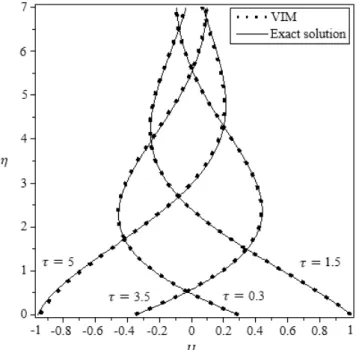
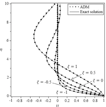
very good agreement between the result of VIM and the exact solution was observed. Fig. 4 and 5 indicate that the difference among ADM and the exact solution are negligible and ADM was converged to the exact solution by increasing iterations.
Fig. 6 confirms the validity of the HPM. As can be seen, HPM completely is similar to exact solution. It may be concluded that HPM methodology is very efficient technique in finding analytical solutions for a wide variety of linear and nonlinear problems. In this article we use the maple package to calculate the functions obtained from VIM, HPM and ADM.
Fig. 2 and 4 illustrate the positive transpiration parameter (injection) which increases the horizontal velocity and negative transpiration parameter (suction), then Fig. 6 has reverse effect since the momentum transmitted to the fluid by the wall which is sucked away.
Fig. 1. A flat plate with oscillating motion, starting from rest, and wall transpiration.
Fig. 2. Comparison of VIM and exact solution in horizontal velocity profile for various values of non-dimensional
Fig. 3. Comparison of VIM and the exact solution in horizontal velocity profile for non-dimensional time
/ 2
, using various transpiration parameter
with a sine excitation of the wall.Fig. 4. Comparison of ADM and exact solution in horizontal velocity profile for various values of non-dimensional
Fig. 5. Comparison of ADM and exact solution in horizontal velocity profile for non-dimensional time
/ 2
, using various transpiration parameter
with a sine excitation of the wall.Fig. 6. Comparison of HPM and the exact solution in horizontal velocity profile for various values of
7. References
[1] Adomian, G., 1992. A review of the decomposition method and some recent results for nonlinear equations, mathematical & computer modeling. 13, 17-43.
[2] Adomian, G., 1994. Solution of physical problems by decomposition, computers & mathematics with applications. 27, 145-154.
[3] Ahmadi, A.R., Zahmatkesh, A., Hatami, M., Ganji, D. D., 2014. A comprehensive analysis of the flow and heat transfer for a nanofluid over an unsteady stretching flat plate, Powder Technology. 258, 125–133.
[4] Almeida Cruz, D.O., Ferreira Lins, E., 2010. The unsteady flow generated by an oscillating wall with transpiration, international journal of non-linear mechanics. 45, 453-457.
[5] Das, S., Jana, M., Guria, M., Janna, R.N., 2008. Unsteady Viscous Incompressible Flow Due to an Oscillating plate in a Rotating Fluid, Journal of Physical Sciences. 12, 51-64.
[6] Domairry, G., Hatami, M., 2014. Squeezing Cu–water nanofluid flow analysis between parallel plates by DTM-Padé Method, Journal of Molecular Liquids. 193, 37-44.
[7] Erdogan, M.E., Imrak, C.E., 2009. On the comparison of the solutions obtained by using two different transform methods for the second problem of stokes for newtonian fluids, International Journal of Non-Linear Mechanics. 44, 27-30.
[8] Ganji, D.D., Afrouzi,G.A., Talarposhti,R.A., 2007. Application of variational iteration method and homotopy perturbation method for nonlinear heat diffusion and heat transfer equations, phys. lett A. 368, 450-457.
[9] Ganji, D.D., HashemiKachapi, S.H., 2011, Analysis of Nonlinear Equations in Fluids,progress in nonlinear science,volume 3, Asian Academic Publisher Limited, Hong Kong, China,pp. 1-294.
[10] Ganji, D.D., Jannatabadi, M., Mohseni, E., 2007. Application of He’s Variational iteration method to nonlinear jaulent-Miodek equations and comparing it with ADM, journal of Computional and applied mathematics. 207, 35-45.
[11] HashemiKachapi, S.H., Barari, A., Tolou, N., Ganji, D.D., 2009. Solution of Strongly nonlinear oscillation systems using Variational approach, Journal of Applied Functional Analysis. 4, 528-535.
[12] Hashemi, S.H., MohammadiDaniali, H.R., Ganji, D.D., 2007. Numerical simulation of the generalized Huxley equation by He’s homotopy perturbation method, Applied Mathematics and Computation. 192, 157-161.
[13] Hatami, M., Ganji, D. D., 2014. Heat transfer and nanofluid flow in suction and blowing process between parallel disks in presence of variable magnetic field, Journal of Molecular Liquids. 190, 159–168.
[14] Hatami, M., Ganji, D. D., 2013. Heat transfer and flow analysis for SA-TiO2 non-Newtonian nanofluid passing through the porous media between two coaxial cylinders, Journal of Molecular Liquids. 188, 155–161.
[15] Hatami, M., Ganji, D. D., 2013. Thermal and flow analysis of microchannel heat sink (MCHS) cooled by Cu– water nanofluid using porous media approach and least square method, Energy Conversion and Management. 78, 347–358.
[16] He, J.H., 1999. Variational iteration method a kind of nonlinear analytical technique: some examples, internat.J.non-linear mech. 34, 699-708.
Nomenclature
u fluid velocity transpiration parameter
t Time η dimensionless axial parameter
Vw transpiration velocity VIM variational iteration method
y axial coordinate λ general lagrangian multiplier
kinematic viscosity HPM homotopy perturbation method
u0 maximum amplitude of wall velocity p embedding parameter
ω frequency of wall the wall velocity ADM adomian’s decomposition method
U dimensionless velocity Ω domain
[17] He, J.H., 1999. Homotopy perturbation technique, computer methods in applied mechanics and engineering. 178, 257-262.
[18] He, J.H., 2004. The homotopy perturbation method for nonlinear oscillators with discontinuities, applied mathematics and computation. 151, 287-292.
[19] He, J.H., 2005. Homotopy perturbation method for bifurcation of nonlinear problems, International Journal of nonlinear science numerical simulation. 6, 207-208.
[20] He, J.H., 2006. Homotopy perturbation method for solving boundary value problems, Physics Letters A. 350, 87-88.
[21] He, J.H., 2007. Variational approach for nonlinear oscillators, Chaos &Solitons and Fractals. 34, 1430-1439. [22] Panton, R., 1968. The transient for Stokes’s oscillating plate a solution in terms of tabulated functions, Journal of Fluid Mechanics. 31, 819–825.
[23] Sheikholeslami, M., Ashorynejad, H.R., Ganji, D. D., Hashim, I., 2012. Investigation of the Laminar Viscous Flow in a Semi-Porous Channel in the Presence of Uniform Magnetic Field using Optimal Homotopy Asymptotic Method, Sains Malaysiana. 41, 1281–1285.
[24] Sheikholeslami, M., Ashorynejad, H.R., Ganji, D. D., Yildirim, A., 2012. Homotopy perturbation method for three-dimensional problem of condensation film on inclined rotating disk, Scientia Iranica B. 19, 437-442.
[25] Sheikholeslami, M., Ganji, D. D., Ashorynejad, H.R., Rokni, H.B., 2012. Analytical investigation of Jeffery-Hamel flow with high magnetic field and nano particle by Adomian decomposition method, Appl. Math. Mech.-Engl. 33, 1553–1564.
[26] Sheikholeslami, M., Ganji, D. D., Rokni, H. B., 2013. Nanofluid Flow in a Semi-Porous Channel in the Presence of Uniform Magnetic Field, IJE TRANSACTIONS C. 26, 653-662.
[27] Sheikholeslami, M., Ganji, D. D., 2013. Heat transfer of Cu-water nanofluid flow between parallel plates, Powder Technology. 235, 873–879.
[28] Sheikholeslami, M., Ganji, D. D., Ashorynejad, H.R., 2013. Investigation of squeezing unsteady nanofluid flow using ADM, Powder Technology. 239, 259–265.
[29] Sheikholeslami, M., Ganji, D. D., 2014. Magnetohydrodynamic flow in a permeable channel filled with nanofluid, Scientia Iranica B. 21, 203-212.
[30] Sheikholeslami, M., Ganji, D. D., 2014. Magnetohydrodynamic flow in a permeable channel filled with nanofluid, Scientia Iranica B. 21, 203-212.
[31] Sheikholeslami, M., Gorji-Bandpy, M., Ganji, D. D., 2013. Numerical investigation of MHD effects on Al2O3– water nanofluid flow and heat transfer in a semi-annulus enclosure using LBM, Energy. 60, 501-510.
[32] Sheikholeslami, M., Gorji-Bandpy, M., Ganji, D. D., 2014. Investigation of nanofluid flow and heat transfer in presence of magnetic field using KKL model, Arabian Journal for Science and Engineering. 39, 5007-5016. [33] Sheikholeslami, M., Gorji-Bandpy, M., Ellahi, R., Zeeshan, A., 2014. Simulation of MHD CuO–water nanofluid flow and convective heat transfer considering Lorentz forces, Journal of Magnetism and Magnetic Materials. 369, 69–80.
[34] Sheikholeslami, M., Gorji-Bandpy, M., Ganji, D. D., 2014. MHD free convection in an eccentric semi-annulus filled with nanofluid, IJST, Transactions of Mechanical Engineering. 38, 217-226.
[35] Sheikholeslami, M., Gorji-Bandpy, M., 2014. Free convection of ferrofluid in a cavity heated from below in the presence of an external magnetic field, Powder Technology. 256, 490–498.
[36] Sheikholeslami, M., Gorji-Bandpy, M., Ganji, D. D., 2014. Lattice Boltzmann method for MHD natural convection heat transfer using nanofluid, Powder Technology. 254, 82-93.