www.biogeosciences.net/12/373/2015/ doi:10.5194/bg-12-373-2015
© Author(s) 2015. CC Attribution 3.0 License.
Coincidences of climate extremes and anomalous vegetation
responses: comparing tree ring patterns to simulated productivity
A. Rammig1, M. Wiedermann1, J. F. Donges1,2, F. Babst3, W. von Bloh1, D. Frank4,5, K. Thonicke1, and M. D. Mahecha6,7
1Earth System Analysis, Potsdam Institute for Climate Impact Research, Telegraphenberg A62, 14412 Potsdam, Germany 2Stockholm Resilience Centre, Stockholm University, Kräftriket 2B, 114 19 Stockholm, Sweden
3Laboratory of Tree-Ring Research, University of Arizona, 1215 E Lowell St, Tucson AZ 85721, USA 4Swiss Federal Research Institute WSL, Zürcherstr. 111, 8903 Birmensdorf, Switzerland
5Oeschger Centre for Climate Change Research, University of Bern, Zähringerstrasse 25, 3012 Bern, Switzerland 6Max Planck Institute for Biogeochemistry, Hans-Knöll-Str. 10, 07745 Jena, Germany
7German Centre for Integrative Biodiversity Research (iDiv) Halle-Jena-Leipzig, Deutscher Platz 5e, 04103 Leipzig,
Germany
Correspondence to:A. Rammig ([email protected])
Received: 28 January 2014 – Published in Biogeosciences Discuss.: 12 February 2014 Revised: 4 November 2014 – Accepted: 5 December 2014 – Published: 20 January 2015
Abstract. Climate extremes can trigger exceptional re-sponses in terrestrial ecosystems, for instance by altering growth or mortality rates. Such effects are often manifested in reductions in net primary productivity (NPP). Investi-gating a Europe-wide network of annual radial tree growth records confirms this pattern: we find that 28 % of tree ring width (TRW) indices are below two standard deviations in years in which extremely low precipitation, high tem-peratures or the combination of both noticeably affect tree growth. Based on these findings, we investigate possibilities for detecting climate-driven patterns in long-term TRW data to evaluate state-of-the-art dynamic vegetation models such as the Lund-Potsdam-Jena dynamic global vegetation model for managed land (LPJmL). The major problem in this con-text is that LPJmL simulates NPP but not explicitly the ra-dial tree growth, and we need to develop a generic method to allow for a comparison between simulated and observed response patterns. We propose an analysis scheme that quan-tifies the coincidence rate of climate extremes with some bi-otic responses (here TRW or simulated NPP). We find a rel-ative reduction of 34 % in simulated NPP during precipita-tion, temperature and combined extremes. This reduction is comparable to the TRW response patterns, but the model re-sponds much more sensitively to drought stress. We identify 10 extreme years during the 20th century during which both
model and measurements indicate high coincidence rates across Europe. However, we detect substantial regional dif-ferences in simulated and observed responses to climatic ex-treme events. One explanation for this discrepancy could be the tendency of tree ring data to originate from climatically stressed sites. The difference between model and observed data is amplified by the fact that dynamic vegetation mod-els are designed to simulate mean ecosystem responses on landscape or regional scales. We find that both simulation re-sults and measurements display carry-over effects from cli-mate anomalies during the previous year. We conclude that radial tree growth chronologies provide a suitable basis for generic model benchmarks. The broad application of coinci-dence analysis in generic model benchmarks along with an increased availability of representative long-term measure-ments and improved process-based models will refine pro-jections of the long-term carbon balance in terrestrial ecosys-tems.
1 Introduction
ecosystem processes exceed their natural range of variabil-ity in the wake of environmental extremes is crucial for an-ticipating the fate of land ecosystems under climate change scenarios (Cotrufo et al., 2011; Jentsch et al., 2011). For in-stance, anomalous ecosystem responses induced by drought events (Schwalm et al., 2012) may decrease the economic returns from forest ecosystems (Hanewinkel et al., 2013) or lead to substantial net CO2 emissions, amplifying climate
change (Reichstein et al., 2013). One prominent example is the 2003 heat wave in Europe, when carbon emissions of
∼0.5 Pg C yr−1were released from forests that usually act as
carbon sinks (Ciais et al., 2005; Janssen et al., 2003). How-ever, it is important to note that extreme events may have differential effects in different biomes, e.g. enhanced vegeta-tion growth during the 2003 heat wave at high elevavegeta-tions in the Alps (Jolly et al., 2005).
Water stress and high temperatures reduce evapotranspi-ration and productivity in many mid- and low-latitude areas (Granier et al., 2007). Yet, the general applicability of such studies is challenged by the different climate responses of forests across biomes and tree species (Babst et al., 2013b; Granier et al., 2007; Lindner et al., 2010). Furthermore, the extent to which increasing amounts of atmospheric CO2may
serve as a buffer against drought by enhancing water use ef-ficiency is being discussed (e.g. Andreu-Hayles et al., 2011; Penuelas et al., 2011; Keenan et al., 2013). The magnitude of these competing effects remains poorly constrained and may differ among tree species or tree age classes (Gedalof and Berg, 2010) and likewise depends on nutrient availabil-ity (e.g. Norby et al., 2010). Another known, yet understud-ied aspect of forest growth dynamics is the role of lagged responses to the previous year’s climate extremes. These can influence current forest productivity, e.g. via decreased nonstructural carbohydrate reserves (e.g. Dietze et al., 2014; Fritts, 1976; Richardson et al., 2013) or altered mortality rates (Bréda et al., 2006; Moreno et al., 2013). Carbon se-questered in the second half of the growing season is gener-ally not used for radial growth but supports a combination of cell-wall thickening and storage (Babst et al., 2014a).
The growing recognition of the role that climate extremes play in land ecosystems (e.g. Williams et al., 2014; Zscheis-chler et al., 2013) and the implications for global carbon cycling requires developing new data analysis tools. While there is a large body of literature on the quantification of extremes in climate variables, we lack techniques to quan-tify extremes in biospheric responses and most importantly a solid framework for linking climatic and biospheric extreme events (Smith, 2011). A suitable methodological approach in this direction requires detecting both instantaneous and lagged responses of a biospheric variable (e.g. tree ring width index – TRW – and net primary productivity – NPP) to cli-matic extremes (e.g. temperature, precipitation or the com-bination of both). We therefore propose a generic method to evaluate the impacts of climate extremes on biospheric variables; this method quantifies the coincidence rates of
extremes in long climatic and biospheric time series (> 50 years). Thereby, we create a unit-free metric that enables us to compare different measures of vegetation productivity. We apply coincidence analysis, a method that was put forward by Donges et al. (2011) in a different context. We exemplify our approach by evaluating a set of European tree ring data and the output from a dynamic vegetation model (LPJmL) model. We focus on exploring the potential of annual radial growth increments (tree ring chronologies) for model eval-uation purposes. This data source is recognized as one of the few opportunities for quantifying ecosystem responses to multiple extreme events on long-term timescales (Babst et al., 2012). Tree ring chronologies can, with certain re-strictions, be regarded as proxies for the variability in stand-scale productivity and offer a possibility to relate long-term tree growth to climate fluctuations and extremes on regional to continental scales (e.g. Babst et al., 2012; Battipaglia et al., 2010). Likewise, tree rings show pronounced lagged ef-fects and a positive relationship with previous fall’s climate (Wettstein et al., 2011). Depending on their sign, climate anomalies in this season may either enhance or mitigate the impact of extremes on forest growth in the subsequent year because they directly affect the growing season length and, related to this, the replenishment of carbon storage (Kuptz et al., 2011). Also, the interaction of carbon accumulation with seed production (i.e. mast years) may sometimes lead to low-growth anomalies regardless of climatic conditions. Such masting events and non-climatic drivers of forest growth (e.g. management or disturbances) may challenge the interpreta-tion of biotic responses to climate extremes because they al-ter carbon allocation patal-terns (Mund et al., 2010). Neverthe-less, tree ring chronologies are widely regarded as robust and very unique long-term indicators of biospheric responses to climate anomalies (Babst et al., 2014b; Jones et al., 2009; Pederson et al., 2014).
Our scale-free approach allows us to directly compare re-sponse patterns identified in the observed tree rings with sim-ulated productivity, which is a straightforward way of testing models for their capacity to reproduce the relevant signatures of extreme impacts in the recent past. Indeed, it has been rec-ognized that it is essential for advanced modelling studies to converge to suitable benchmarks for testing terrestrial bio-sphere models (cf. Dalmonech and Zaehle, 2013; Kelley et al., 2013; Luo et al., 2012).
For instance, Luo et al. (2012) conclude that suitable model benchmarks are characterized by “objectivity, effec-tiveness, and reliability for evaluating model performance”. Hence, the goal has to be a suite of metrics that can em-brace characteristic response functions. Along these lines, our study evaluates the potential of the coincidence analysis framework to become an element of a generic model bench-marking system. We address this issue by working on the following specific questions:
– do state-of-the-art dynamic vegetation models agree with observed responses to climate extremes?
– how can long-term observations help us understanding biotic responses to extreme events?
2 Materials and methods 2.1 Observed and modelled data 2.1.1 Measurements of tree ring widths
We compiled TRW chronologies from 606 sites across Eu-rope and parts of northern Africa (10◦W–40◦E, 30◦–70◦N).
These data represent a subset of the European tree ring net-work (Babst et al. 2013; see http://onlinelibrary.wiley.com/ doi/10.1111/geb.12023/suppinfo), which includes measure-ments from 36 tree species. We grouped sites into three categories: common needle-leaved species (e.g. Larix
de-cidua, Picea abies, Pinus Syvestris, Abies alba; 116 sites),
broadleaved species (e.g. Fagus silvatica, Quercus robur,
Quercus petraea; 378 sites) and other species (mainly
Mediterranean conifers; 112 sites). For the detection of growth extremes, low frequency variability including the bi-ological age/size trend characteristic of tree ring data was removed from the constituent tree ring time series at each site using a spline detrending with a 50 % frequency cut-off response at 30 years (Babst et al., 2012). Prior to de-trending, the variance of each time series was stabilized us-ing an adaptive power transformation as described by Cook and Peters (1997) and the mean tree ring chronologies were corrected for changes in sample replication (Frank et al., 2007) to reduce biases in the detection of growth extremes induced by variance changes over time. The tree ring de-trending and standardization procedure converts the tree ring width data into dimensionless indices (so-called tree ring
width indices, TRWs) with a mean of approximately unity. The tree ring data set spans most of terrestrial Europe, but is not evenly distributed across the continent (see Babst et al., 2013, and Fig. 3). Conifer sites are most frequent in Scandi-navia, in the Alpine region and in the Mediterranean, while broadleaved species are predominantly located in central Eu-rope and northern Spain (Babst et al., 2013).
2.1.2 Climate data
We use the WATCH-ERA-Interim (European global atmo-spheric Re-Analysis data from the Water and Global Change EU-Project) daily climate data at 0.25 latitude/longitude res-olution based on downscaled WATCH climate data (Wee-don et al., 2011) for the years 1901–2001 and extended to 2010 using downscaled ERA-Interim climate data (Dee et al., 2011). Daily temperature, precipitation and solar radia-tion were used to drive the model runs. For the coincidence analysis with TRW and simulated NPP, we calculate mean annual temperature (T) and annual precipitation sums (P) over the growing season from the climate data set (see be-low).
2.1.3 Simulated net primary productivity (NPP)
Simulations of monthly NPP are performed with the dynamic global vegetation model LPJmL (Bondeau et al., 2007; Sitch et al., 2003) with a fully coupled carbon and water cycle (Gerten et al., 2004). The model is driven by temperature, radiation, precipitation and atmospheric CO2concentration.
The productivity of vegetation (GPP) for each plant func-tional type (PFT) is simulated by a process-based photo-synthesis scheme based on Farquhar (Farquhar et al., 1980) that adjusts carboxylation capacity and leaf nitrogen season-ally and within the canopy profile (Haxeltine and Prentice, 1996). Net primary production (NPP) is derived by subtract-ing maintenance and growth respiration from GPP. LPJmL simulates the allocation of accumulated carbon to the plant’s compartments (leaves, stem, root and reproductive organs) according to allometric constraints. Responses of the mod-elled vegetation to climate extremes include the inhibition of photosynthesis and increased maintenance respiration at high temperatures and reduced stomatal conductance and thus re-duced photosynthesis with water stress.
For the present study, we ran LPJmL in its natural veg-etation mode not considering land management and land-use change. Process-based simulation of fire is included by the so-called SPITFIRE model, which is coupled to LPJmL (Thonicke et al., 2010). Simulation runs were performed at 0.25◦×0.25◦spatial resolution based on the
WATCH-ERA-Interim daily climate data. A global value of annual atmo-spheric CO2concentration was prescribed for the 1901–2010
30 years of the climate drivers in order to obtain equilibrium carbon pools and fluxes and vegetation cover. Model param-eterization and soil types followed Gerten et al. (2004) and Sitch et al. (2003).
2.1.4 Determination of the growing season for TRW and simulated NPP
To determine the length of the growing season (GSobs),
we use the fraction of photosynthetically absorbed radiation (FAPAR) derived from remote sensing and interpolated to daily values (from the Moderate-resolution Imaging Spectro-radiometer (MODIS) Pinty et al., 2011) at each geographical coordinate of a tree ring time series. The MODIS-TIP (two-stream inversion package) provides broadband albedo values resulting in time series that are comparable across vegetation types. Given that there is no commonly accepted approach to derive growing season length from remote sensing observa-tions via a threshold approach (see, e.g., White et al., 2009), we apply a mixture of absolute and relative heuristic criteria. First, we flagged days as non-growing season when FAPAR values drop below 0.12 or are below −0.8 standard devia-tions of FAPAR. To ensure that the second criterion does not affect evergreen sites, we reset all values > 0.43 to growing season. Importantly, we considered only the longest phase of points that follow these criteria to be GSobs, and we only
al-low for one single GSobsin Europe as we assume that double
growing seasons do not play a substantial role in the lati-tudes under scrutiny. The dynamic definitions of the GSobs
derived from FAPAR allow deriving typical growing seasons at each geographical point, thereby assuming that the aver-age climate data for these days of the year are robust proxies for the growing season throughout the entire observational period.
To determine the length of the growing season for each simulated grid cell (GSsim), we use the simulation results for
NPP. As GSsim we define here the longest period of
subse-quent months per year when the monthly NPP is greater than 0.
2.1.5 Preprocessing of climate data, TRW and simulated NPP for coincidence analysis
The coincidence analysis requires pairing each point in the TRW data set with local T andP variability. Accordingly, each TRW site is associated with the site-specific (i.e. geo-graphically encompassing) climate grid cell of the WATCH-ERA-Interim data at 0.25◦×0.25◦spatial resolution. In this
way, we obtain 606 pairs of time series representing tree ring growth and climatological data. Monthly temperature and precipitation data are averaged and summed, respectively, over the growing season (see Sect. 2.1.5). The maximum temporal overlap between each pair of time series determines the length of the period for coincidence analysis.
To obtain pairs of time series for the comparison of sim-ulated NPP withP andT in a comparable way as for TRW, we calculate the sum of simulated NPP over the growing sea-son (see Sect. 2.1.5). Analogously to the coincidence analy-sis between TRW and climate data, we compute the average temperature and total precipitation over the growing season, where NPP > 0. We obtain pairs of simulated NPP and cli-mate drivers for each grid cell.
The TRW data set consists of 606 time series at selected measurement sites throughout Europe. For comparison with simulated NPP, we select the corresponding grid cell centres nearest to the measurement sites.
2.2 Coincidence analysis and definition of extreme events
For our analysis, we search for coincidences (Donges et al., 2011) between specific percentiles in the pairs of biotic and climate time series. In the case of TRW and NPP, values smaller than the 10th percentiles were used (low-productivity extremes). In the climate records, all values exceeding the 90th percentiles of mean growing season temperature (hot extremes) and being less than the 10th percentile of the to-tal growing season precipitation (dry extremes) were defined as extreme events. This combination of climatic and biotic extremes tests the link between extremely high temperature, low precipitation or the combination of both in causing low-growth responses at all sites. At alpine or boreal sites, partic-ularly high temperatures may even lead to better growth con-ditions (e.g. Jolly et al., 2005). Similarly, extremely low tem-peratures during the growing season could cause low-growth extremes, e.g. in the Alps or the boreal zone (e.g. Babst et al., 2012). We therefore interpret our results carefully regarding these issues.
Precipitation (mm/yr) A)
400
600
800
I I I I I
L L P
10% quantile P extreme
T
ree r
ing width inde
x B)
0.4
0.8
1.2
1.6
1900 1905 1910 1915 1920 1925 1930 1935 1940 1945 1950 1955 1960 1965 1970 1975 1980 1985 1990 1995 2000 2005 2010
TRW 10% quantile TRW extreme
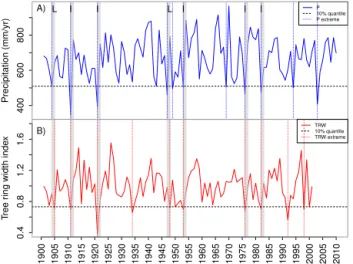
Figure 1.Example of coincidence analysis between a time series
of(a)precipitation (P) and(b)tree ring width indices (TRW). The dashed horizontal line represents the lower 10 % quantile. Events in precipitation or tree ring width that fall below this threshold are counted as extreme events, as indicated by the dotted vertical lines forP (blue) and TRW (red). Grey bars indicate the coinci-dence of extreme P and TRW events within a time window of 2 years (1t=2) and are counted as one coincidence. In this exam-ple, we count 11 climate extremes and 7 coincidences with TRW for1t=2, resulting in a coincidence rate ofr=7/11=0.64. Note that if there are two TRW extremes coinciding with oneP extreme in the time window of1t=2, this would account for only one ex-treme. The letters “I” and “L” indicate instantaneous and lagged effects (i.e. carry-over effects), respectively. When setting the time window to1t=1 andτ=0, five coincidences are counted and for 1t=1 andτ=1, two coincidences are counted in this example.
or combinedP andT to obtain the coincidence raterwith 0≤r≤1 (0 if no coincidences occur and 1 if the maximum number of possible coincidences occurs).
2.3 Testing the significance of coincidences
Autocorrelations as well as the specific shape of the distribu-tion of amplitudes in the considered climatological and biotic time series can have a profound influence on the observed bi-variate coincidence rates. To control for these effects and as-sess the statistical significance of the computed coincidence ratesr, we create 1000 iAAFT (iterative Amplitude Adjusted Fourier Transformation; Schreiber and Schmitz, 2000; Ven-ema et al., 2006) surrogate time series for each site and grid cell. The iAAFT surrogates are fully statistically indepen-dent from the original time series but characterized by the same amplitude distribution and, most importantly, the same autocorrelation properties. Hence, we can investigate the co-incidence rate of extremes that would be expected to arise by chance between two time series of a given autocorrelation structure. We calculate for each site and grid cell the distribu-tion of the coincidence rates of the iAAFT surrogate time se-ries. The coincidence rater(calculated from climate and
bi-otic extremes) is assumed to be significant if it is higher than the 90 % percentile of the surrogate distribution. In the fol-lowing analysis, we only consider TRW sites and simulated grid cells with a significant coincidence rater. For brevity, these locations are subsequently addressed as significant sites or grid cells.
2.4 Detection of European-wide extreme years
To identify years with a pronounced European-wide forest response to climate extremes, i.e. years that yield a high num-ber of coincidences across the continent, we take the sum over all coincidences at significant sites/grid cells occurring during a specific year and divide it by the number of all sig-nificant sites/grid cells, again yielding a number between 0 and 1 (0 if no coincidences occur at significant sites/grid cells and 1 if all significant sites show a coincidence in the year considered). As “European-wide extreme years” we define all values one standard deviation above the average annual significant coincidence rate.
2.5 Analysis of downregulation of forest growth by extreme events
To estimate the potential downregulation of forest growth by extreme events, we assume that years with coincidences of extremes inP,T and combinedP andT with TRW and NPP represent extreme years for the ecosystem. For this analysis, the TRW and NPP time series were rescaled to zero mean and unit variance (z-scores) in order to guarantee comparability in the summary statistics (note that the coincidence analysis itself is scale free and does not require this preprocessing step). We then selectz-scored TRW and NPP values during extreme years, i.e. during years with significant coincidences between extreme response and extreme climate. We calculate the proportion ofz-scored NPP and TRW values duringP, T andP andT extremes below two standard deviations in relation to the total number of TRW and NPP extremes.
3 Results and Discussion
In this section we first discuss the general picture of the im-pact of climate extremes on measured TRW and modelled NPP and then focus on patterns of spatial and temporal coin-cidence rates at significant sites/grid cells.
a) TRW and P extremes
Frequency
−6 −4 −2 0 2
0
50
100
150
200
250
300
350 TRWext< −2 σ
8.59%
b) TRW and T extremes
Frequency
−6 −4 −2 0 2
0
50
100
150
200
250
300
350 TRWext< −2 σ
6.13%
c) TRW and T&P extremes
Frequency
−6 −4 −2 0 2
0
50
100
150
200
250
300
350 TRWext< −2 σ
13.13%
d) NPP and P extremes
Frequency
−6 −4 −2 0 2
0
50
100
150
200
250
300
350 NPPext< −2 σ
20.25%
e) NPP and T extremes
Frequency
−6 −4 −2 0 2
0
50
100
150
200
250
300
350 NPPext< −2 σ
3.02%
f) NPP and T&P extremes
Frequency
−6 −4 −2 0 2
0
50
100
150
200
250
300
350 NPPext< −2 σ
10.8% Deviation of growth during extreme years in units of standard deviation (z-scores)
Deviation of growth during extreme years in units of standard deviation (z-scores)
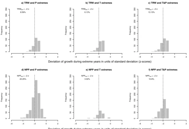
Figure 2.Histograms of deviations of growth responses of TRW(a, b, c)and NPP(d, e, f)during extreme years in units of standard deviations
(z-scores). The vertical dashed grey line marks two negative standard deviations. The numbers denote the proportion of coinciding events below two standard deviations (see also Table S1 in the Supplement).
TRW
NPP
TRW
NPP
TRW
NPP
Years 1901 1902 1903 1904 1905 1906 1907 1908 1909 1910 1911 1912 1913 1914 1915 1916 1917 1918 1919 1920 1921 1922 1923 1924 1925 1926 1927 1928 1929 1930 1931 1932 1933 1934 1935 1936 1937 1938 1939 1940 1941 1942 1943 1944 1945 1946 1947 1948 1949 1950 1951 1952 1953 1954 1955
TRW
NPP
TRW
NPP
TRW
NPP
Years 1956 1957 1958 1959 1960 1961 1962 1963 1964 1965 1966 1967 1968 1969 1970 1971 1972 1973 1974 1975 1976 1977 1978 1979 1980 1981 1982 1983 1984 1985 1986 1987 1988 1989 1990 1991 1992 1993 1994 1995 1996 1997 1998 1999 2000 2001 2002 2003 2004 2005 2006 2007 2008 2009 2010
P
T&P
P
T&P
T
T
Figure 3.Extreme years during the period 1901–2010 as detected by the coincidence analysis for TRW and NPP (only at TRW sites) with
values are below two (one) standard deviations in years with extremely high temperatures, low precipitation and com-bined temperature and precipitation extremes, respectively (Fig. 2a, b, c, Table S1). At TRW sites, 1491 extremes in simulated NPP are detected. The higher number of detected NPP extremes may partially reflect the fact that the same cli-mate forcing data are used to drive NPP simulations (result-ing in a higher probability of coincidences between climate and NPP extremes than coincidences between climate and TRW extremes). Of the simulated NPP values at TRW sites, 20, 3 and 11 % (56, 10 and 27 %) are below two (one) stan-dard deviations in years withP,T and combinedP andT extremes, respectively (Fig. 2d, e, f, Table S1). The strong re-duction in simulated NPP during precipitation extremes may be related to an overestimation of the modelledP sensitivity of NPP (Babst et al., 2013; Beer et al., 2010). Our definition focusses on extremes during the growing season and thereby neglects any impacts of extreme events that occur outside the growing season which could have significant impact on forest productivity, such as respiratory carbon losses in autumn and winter depleting carbon storage pools, and reduce growth in the following year (e.g. Piao et al., 2008). Extremely warm temperatures in winter may also increase the snow amount in the boreal zone, leading to a delayed start of the next grow-ing season (Helama et al., 2013). By contrast, warm win-ter/spring temperatures are beneficial for an earlier start of the next growing season (Polgar and Primack, 2011; Rossi et al., 2014). Keeping this in mind, our results for growing sea-son extremes (Fig. 2) suggest that TRW and simulated NPP show subtle differences in their response to different climate extremes and that the seasonality of climate anomalies may be of vital importance in this respect. Hence, in the follow-ing, we carry out an in-depth investigation as to how these differences can be attributed.
3.2 Extreme years as determined from coincidences across Europe
To analyse the responses of forest growth to drought and heat extremes in models and observations, it is necessary to first evaluate whether the timing of the climate-driven reductions in TRW and simulated NPP events match reasonably well. In this context, we determine European-wide extreme years as described in Sect. 2.4. For both TRW and simulated NPP, we identify the years 1911, 1921, 1945, 1947, 1976 and 2003 (Fig. 3, dark grey boxes) as dry extremes with substantial bi-otic impacts. Extremely hot years are detected in 1934, 1945, 1947, 1949, 1950, 2002 and 2003 (Fig. 3). Coincidences of combined P andT extremes with NPP and TRW are de-tected in 1945, 1947, 1994 and 2003 (Fig. 3). These results are in good agreement with earlier studies that identified ex-treme events during these years. In their analysis, Babst et al. (2012) show that 1947 had extremely low growth in south-ern, southeastern and central Europe due to dry conditions. Neuwirth et al. (2007) reveal 1921 as a negative extreme
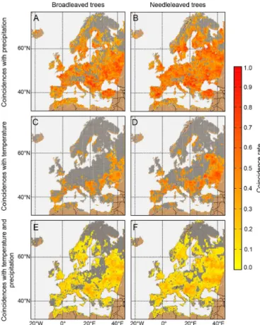
Figure 4.Map of coincidence rates between extremes in simulated
NPP and precipitation for(a)broadleaved and(b) needle-leaved trees. Coincidence rates between extremes in simulated NPP and temperature for(c)broadleaved and(d)needle-leaved trees. Coinci-dence rates for simulated NPP and combined precipitation and tem-perature extremes for(e)broadleaved and(f)needle-leaved trees. The colour bar gives the coincidence raterfor the coincidence anal-ysis with1t=2. Only grid cells with significant coincidence rates are coloured; nonsignificant grid cells are marked in grey. Note that the significance level for each grid cell is determined separately.
year in the Rhône Valley, Jura, northern Bavaria and north-ern Germany and 1947 as a negative extreme year in west-ern Poland, northwestwest-ern Germany and Slovenia. Battipaglia et al. (2010) reconstructed temperature extremes from tree rings and found extremely warm conditions in 1911, 1921, 1964 and 2003. Extreme fire years are reported in 1947 and 1976 in Germany (Goldammer, 2001). In 1994, temperature anomalies of up to 2◦C in comparison to 1961–1990 were
recorded throughout Europe (Halpert et al., 1995). The ef-fects of the extreme year 2003 in Europe are well known (e.g. Ciais et al., 2005). This list demonstrates the capability of our coincidence analysis to identify European-wide heat and drought extremes.
3.3 Spatial distribution of responses to extreme events
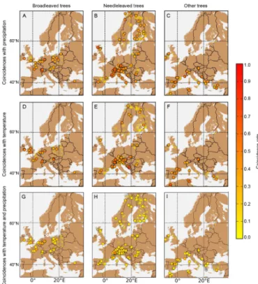
Figure 5.Map of tree ring sites and coincidence rates at each site. Coincidence rates between extremes in TRW and precipitation for
(a) broadleaved,(b) needle-leaved and(c)other tree species are provided. In the middle row (d, e, f), coincidence rates between extremes in TRW and temperature for the different tree species are displayed. In the lower row(g, h, i), coincidence rates for extremes in TRW and combined precipitation and temperature extremes are given. Nonsignificant sites are marked with transparent dots. The colour bar gives the coincidence raterfor the coincidence analysis with1t=2.
of tree ring records as model benchmarks under climate ex-tremes will depend crucially on the matches in these spatial patterns. Figure 4 identifies areas where simulated NPP of broadleaved and needle-leaved trees shows significant coin-cidences with precipitation, temperature and combined tem-perature and precipitation extremes, respectively. Figure 5 shows the analogue picture for TRW. Generally, we find more significant grid cells with high coincidence rates be-tween simulated NPP and precipitation (n=259 in grid cells at TRW site) than with temperature extremes (n=74 in grid cells at TRW site; Fig. 4 upper row) during the growing sea-son. As mentioned before, this may be related to an overes-timation of the modelledP sensitivity of NPP. It also shows that water is an important driver at many sites particularly un-der extreme conditions (Reichstein et al., 2013; Zscheischler et al., 2014c). For the observed TRW values, we find almost the same amount of significant sites for coincidences withP (n=189) as for coincidences with T (n=139; Fig. 5). In contrast to observed TRW, simulated NPP displays generally low or insignificant coincidence rates with high -temperature and low-precipitation extremes in mountainous areas (Figs. 4
5 10 15 20 5 10 15 20
Temperature in 2.5°C bins
Mean coincidence rate
A B
0.1 0.2 0.3 0.4 0.5 0.6
TRW
Simulated NPP at TRW sites
Temperature in 2.5°C bins
5 10 15 20
Temperature in 2.5°C bins
C
1
13 12 11 16
37 21
5 1
1
2 1
10 19
23 12
3 1
13 26
34 49
7631 10 2
1
8 19
12 28 40 6 4
1 1 2 9 27
39 18
5
1
1 16
30 40
52 76 17 8 1
Figure 6.Significant coincidence rates of TRW (red dots) and
sim-ulated NPP at TRW sites (blue dots) with(a)precipitation,(b) tem-perature, and (c) the combination of both, in climate space (as given in 2.5◦C temperature bins,x axis) averaged over all tree
species. Sites/ grid cells with significant coincidences are aggre-gated in 2.5◦C mean annual temperature bins. Error bars give the
standard deviation among sites/grid cells, and numbers in the plot denote the n of significant sites/grid cells for each 2.5◦C
tempera-ture bin (numbers for TRW in red and for simulated NPP in blue). Note that for some bins, for TRW or site NPP only one value exists.
and 5). This may be due to the spatial resolution of the cli-mate data, where grid cells cannot resolve climatic differ-ences along steep altitudinal gradients in the Alps and the related responses displayed by TRW (e.g. King et al., 2013). Climate extremes (low precipitation, high temperatures) in such areas may therefore not limit simulated NPP during the growing season. This calls for higher-resolution long-term climate data sets (or ideally a denser network of climate sta-tions in complex terrain) to better capture site-level climate extremes and improve their representation in simulated NPP anomalies.
Drought conditions may not only result from a lack of rainfall but also from high temperature, which drives vapour pressure deficit in dry areas such as the Mediterranean region (Williams et al., 2012). Therefore, we also show the coinci-dence ratesr for the combinedP andT extremes (Figs. 4 and 5, lower row). A characteristic feature is that these coin-cidence rates are generally lower because combinedP andT events are rare. However, we find a relatively high number of significant grid cells with combined events (n=243 in grid cells at TRW site,n=242 for TRW out of 606 TRW sites).
0.2 0.4 0.6 0.8 0.2 0.4 0.6 0.8 0.2
0.8
0.6
0.4 0.2 0.8
0.6
0.4
NPP at TRW sites TRW
Coincidences with precipitation
Coincidences with temperature
Coincidence rate for ΔT=1, �=0 Coincidence rate for ΔT=1, �=0
Coincidence rate for
Δ
T=1,
�
=1
Coincidence rate for
Δ
T=1,
�
=1
0.2 0.8
0.6
0.4
Coincidences with temperature and
precipitation
Coincidence rate for
Δ
T=1,
�
=1
A B
C D
E F
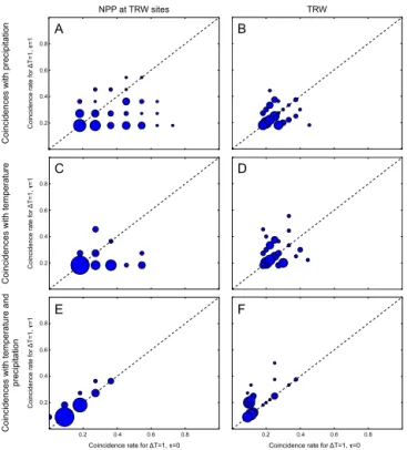
Figure 7.Instantaneous (rcalculated for1t=1 andτ=0,xaxis)
vs. lagged (rcalculated for1t=1 andτ=1,yaxis) coincidences of extreme events. The size of the dots is proportional to the amount of significant coincidences, i.e. larger dots indicate a higher number of sites/grid cells with significant coincidences. Note that the reg-ular grid of coincidence rates results from consistent time series length for simulated NPP, while the length of the time series for TRW differs.
in low-temperature zones and higher r in high-temperature zones (Fig. 6, blue dots). The coincidence rates between sim-ulated NPP and P range from r≈0.38 to 0.54 (Fig. 6a); for NPP andT they scatter around∼0.4 (Fig. 6b), whereas for both NPP and TRW and combinedT andP extremes,r ranges between 0.1 and 0.2 (Fig. 6c). Again, the overestima-tion of theP sensitivity of simulated NPP in comparison to TRW is visible. TRW displays rather constant coincidence rates of ∼0.4 with T (Fig. 6a, red dots) and P (Fig. 6b) along the temperature gradient, whereas for combined ex-tremes the increase in the coincidence rates is similar to that of NPP (Fig. 6c). The lower coincidence rates in TRW may be driven by adverse effects of extremeT, e.g. in mountain-ous areas, where high temperatures during the growing sea-son may even lead to increased growth (Jolly et al., 2005). Also, the importance of nonstructural carbohydrates (NSCs) should not be underestimated. NSCs can be stored for up to 10 years, used as resources during unfavourable growth con-ditions, and thereby buffer the negative effects of extreme events (e.g. Carbone et al., 2013; Richardson et al., 2013; Klein et al., 2014). The low coincidence rates of NPP and TRW with combined T andP extremes again result from the rareness of these events (Fig. 6c).
3.4 Instantaneous and lagged responses to extreme events
To further assess the growth responses to climate extremes found in models and observations, it is necessary to analyse their dynamics. Lagged biotic responses to extreme events are of particular interest. We therefore compare the coinci-dence rater in the same year (i.e. instantaneous responses, calculated with1t=1 andτ=0) with the coincidence rate in the year after the climate extreme (i.e. lagged responses, calculated with1t=1 andτ=1; Fig. 7 and see also Fig. 1).
We find a high number of coincidences in the year after the extreme compared to the instantaneous response, par-ticularly during combined P and T extremes, indicating lagged responses (Fig. 7e, f). Overall, negative precipita-tion anomalies combined with positive temperature extremes lead to reduced growth not only in the current, but also in the following year. This is in line with other studies (e.g. Babst et al., 2012; Franke et al., 2013) that have empha-sized the importance of considering lagged effects in mea-sured TRW. Babst et al. (2012) found that particularly late growing season extremes lead to reduced growth in the fol-lowing year. The pattern is less pronounced in simulated NPP (Fig. 7e). In the model, lagged effects in NPP are simulated when unfavourable climate conditions lead to low produc-tivity and high respiration costs during the current year and thus less accumulation of biomass. Constant or less accu-mulated biomass then leads to reduced siaccu-mulated NPP dur-ing the followdur-ing year. Because simulated NPP represents a rather short-term measure of carbon use compared to ob-served TRW, it responds more instantaneously to changes in photosynthesis and respiration during extreme events. In contrast, observed TRW integrates carbon accumulation and growth over a whole growing season, relies in part on stored carbohydrates, and may even be influenced by longer-term responses to canopy and root architecture. These considera-tions may explain some of the observed differences between TRW and simulated NPP under extreme climate conditions.
4 Conclusions
We present a simple method for detecting impacts of ex-treme events in time series of climate and forest growth that is based on coincidence analysis. The coincidence metric is viewed as a “unit-free”, neutral measure for biotic responses to climate impacts. The method is general and independent of units and does not require attempts to convert tree ring width to NPP for comparison with model output; instead, we can compare the results of the coincidence analysis to test for possible causal relationships between extreme climate and extreme growth responses.
extreme events and, thus, for evaluating dynamic vegetation models. Our study shows that low precipitation, high tem-perature and combined extremes lead to substantial losses in forest productivity, which is∼30 % below two standard de-viations during extreme years. We identified years with cli-mate extremes which caused extreme ecosystem responses in Europe for the 20th century, which are consistent with previ-ously reported evidence.
Our study has shown the potential of standardized tree ring data to be used for the evaluation of dynamic global vegeta-tion models abilities to simulate growth responses to climate extremes. Earlier model evaluation studies have lacked this type of analysis. As climate extremes can have long-lasting impacts, DGVMs need to be able to simulate such effects and capture the processes that are responsible for multiyear lagged effects. The combination of improved DGVMs and the method of coincidence analysis can then be applied to quantify the impacts of extreme events, e.g. on the long-term fate of the global carbon balance.
The Supplement related to this article is available online at doi:10.5194/bg-12-373-2015-supplement.
Acknowledgements. This work emerged from the
CARBO-Extreme project (grant agreement no. 226701) of the European Community’s 7th framework program. M. Wiedermann has been supported by the German Federal Ministry for Science and Education via the BMBF Young Investigators Group CoSy-CC2 (grant no. 01LN1306A). M.D. Mahecha acknowledges support by the GEOCARBON project (grant agreement no: 283080) of the European Community’s 7th framework program. J.F. Donges thanks the German National Academic Foundation and the Stordalen Foundation for financial support. F. Babst acknowl-edges funding from the Swiss National Science Foundation (grant PBSKP2_144034). We thank two anonymous reviewers for their constructive comments to the manuscript.
Edited by: C. A. Williams
References
Andreu-Hayles, L., Planells, O., Gutierrez, E., Muntan, E., Helle, G., Anchukaitis, K. J., and Schleser, G. H.: Long tree-ring chronologies reveal 20th century increases in water-use effi-ciency but no enhancement of tree growth at five Iberian pine forests, Glob. Change Biol., 17, 2095–2112, doi:10.1111/j.1365-2486.2010.02373.x, 2011.
Babst, F., Carrer, M., Poulter, B., Urbinati, C., Neuwirth, B., and Frank, D.: 500 years of regional forest growth variability and links to climatic extreme events in Europe, Environ. Res. Lett., 7, 045705 doi:10.1088/1748-9326/7/4/045705, 2012.
Babst, F., Poulter, B., Trouet, V., Tan, K., Neuwirth, B., Wilson, R., Carrer, M., Grabner, M., Tegel, W., Levanic, T., Panayotov,
M., Urbinati, C., Bouriaud, O., Ciais, P., and Frank, D.: Site-and species-specific responses of forest growth to climate across the European continent, Glob. Ecol. Biogeogr., 22, 706–717, doi:10.1111/geb.12023, 2013.
Babst, F., Bouriaud, O., Papale, D., Gielen, B., Janssens, I. A., Nikinmaa, E., Ibrom, A., Wu, J., Bernhofer, C., Koest-ner, B., Gruenwald, T., Seufert, G., Ciais, P., and Frank, D.: Above-ground woody carbon sequestration measured from tree rings is coherent with net ecosystem productivity at five eddy-covariance sites, New Phytol., doi:10.1111/nph.12589, 1289– 1303, 2014a.
Babst, F., Alexander, M. R., Szejner, P., Bouriaud, O., Klesse, S., Roden, J., Ciais, P., Poulter, B., Frank, D., Moore, D. J. P., and Trouet, V.: A tree-ring perspective on the terrestrial carbon cycle, Oecologia, 176, 307–322, 2014b.
Barriopedro, D., Fischer, E. M., Luterbacher, J., Trigo, R., and Garcia-Herrera, R.: The Hot Summer of 2010: Redrawing the Temperature Record Map of Europe, Science, 332, 220–224, doi:10.1126/science.1201224, 2011.
Battipaglia, G., Frank, D., Büntgen, U., Dobrovolny, P., Bradzdil, R., Pfister, C., and Esper, J.: Five centuries of Central European temperature extremes reconstructed from tree-ring density and documentary evidence, G. Planet. Change, 72, 182–191, 2010. Beer, C., Reichstein, M., Tomelleri, E., Ciais, P., Jung, M.,
Carval-hais, N., Rödenbeck, C., Arain, M. A., Baldocchi, D., Bonan, G. B., Bondeau, A., Cescatti, A., Lasslop, G., Lindroth, A., Lomas, M., Luyssaert, S., Margolis, H., Oleson, K. W., Roupsard, O., Veenendaal, E., Viovy, N., Williams, C., Woodward, F. I., and Pa-pale, D.: Terrestrial Gross Carbon Dioxide Uptake: Global Dis-tribution and Covariation with Climate, Science, 329, 834–838, 2010.
Bondeau, A., Smith, P. C., Zaehle, S., Schaphoff, S., Lucht, W., Cramer, W., Gerten, D., Lotze-Campen, H., Müller, C., Reich-stein, M., and Smith, B.: Modelling the role of agriculture for the 20th century global terrestrial carbon balance, Glob. Change Biol., 13, 679–706, 2007.
Bréda, N., Huc, R., Granier, A., and Dreyer, E.: Temperate forest trees and stands under severe drought: a review of ecophysiologi-cal responses, adaptation processes and long-term consequences, Ann. For. Sci., 63, 625–644, 2006.
Carbone, M. S., Czimczik, C. I., Keenan, T., Murakami, P., Peder-son, N., Schaberg, P. G., Xu, X., and RichardPeder-son, A. D.: Age, allocation and availability of nonstructural carbon in mature red maple trees, New Phytol., 200, 1145–1155, 2013.
Ciais, P., Reichstein, M., Viovy, N., Granier, A., Ogée, J., Allard, V., Aubinet, M., Buchmann, N., Bernhofer, C., Carrara, A., Cheval-lier, F., De Noblet, N., Friend, A. D., Friedlingstein, P., Grün-wald, T., Heinesch, B., Keronen, P., Knohl, A., Krinner, G., Lous-tau, D., Manca, G., Matteucci, G., Miglietta, F., Ourcival, J. M., Papale, D., Pilegaard, K., Rambal, S., Seufert, G., Soussana, J. F., Sanz, M. J., Schulze, E.-D., Vesala, T., and Valentini, R.: Europe-wide reduction in primary productivity caused by the heat and drought in 2003, Nature, 437, 529–533, 2005.
Cook, E. R. and Peters, K.: Calculating unbiased tree-ring in-dices for the study of climatic and environmental change, The Holocene, 7, 361–370, 1997.
dynam-ics in a Mediterranean woodland, Biogeosciences, 8, 2729–2739, doi:10.5194/bg-8-2729-2011, 2011.
Dalmonech, D. and Zaehle, S.: Towards a more objective evalua-tion of modelled land-carbon trends using atmospheric CO2and
satellite-based vegetation activity observations, Biogeosciences, 10, 4189–4210, doi:10.5194/bg-10-4189-2013, 2013.
Dee, D. P., Uppala, S. M., Simmons, A. J., Berrisford, P., Poli, P., Kobayashi, S., Andrae, U., Balmaseda, M. A., Balsamo, G., Bauer, P., Bechtold, P., Beljaars, A. C. M., van de Berg, L., Bid-lot, J., Bormann, N., Delsol, C., Dragani, R., Fuentes, M., Geer, A. J., Haimberger, L., Healy, S. B., Hersbach, H., Holm, E. V., Isaksen, L., Kallberg, P., Kohler, M., Matricardi, M., McNally, A. P., Monge-Sanz, B. M., Morcrette, J. J., Park, B. K., Peubey, C., de Rosnay, P., Tavolato, C., Thepaut, J. N., and Vitart, F.: The ERA-Interim reanalysis: configuration and performance of the data assimilation system, Q. J. Roy. Meteor. Soc., 137, 553–597, doi:10.1002/qj.828, 2011.
Dietze, M. C., Sala, A., Carbone, M. S., Czimczik, C. I., Mantooth, J. A., Richardson, A. D., and Vargas, R.: Nonstructural Carbon in Woody Plants, Annu. Rev. Plant Biol., 65, 667–687, 2014. Donges, J. F., Donner, R. V., Trauth, M. H., Marwan, N.,
Schellnhuber, H. J., and Kurths, J.: Nonlinear detection of paleoclimate-variability transitions possibly related to hu-man evolution, P. Natl. Acad. Sci. USA, 108, 20422–20427, doi:10.1073/pnas.1117052108, 2011.
Farquhar, G. D., von Caemmerer, S., and Berry, J. A.: A biochem-ical model of photosynthesic CO2assimilation in leaves of C3
plants, Planta, 149, 78–90, 1980.
Field, C. B., Barros, V., Stocker, T. F., and Dahe, Q.: Special Re-port on Managing the risks of Extreme Events and Disasters to Advance Climate Change Adaptation (SREX), Cambridge Uni-versity Press, 237 pp., 2012.
Frank, D., Esper, J., and Cook, E.: Adjustment for proxy number and coherence in large-scale temperature reconstruction, Geo-phys. Res. Lett., 34, L16709, doi:10.1029/2007GL030571, 2007. Franke, J., Frank, D., Raible, C. C., Esper, J., and Brönnimann, S.: Spectral biases in tree-ring climate proxies, Nature Climate Change, 3, 360–364, 2013.
Fritts, H. C.: Tree Rings and Climate, Academic Press, London, 156–202, 1976.
Gedalof, Z. and Berg, A. A.: Tree ring evidence for limited direct CO2 fertilization of forests over the 20th century, Glob. Bio-geochem. Cy., 24, Gb3027, doi:10.1029/2009gb003699, 2010. Gerten, D., Schaphoff, S., Haberlandt, U., Lucht, W., and Sitch, S.:
Terrestrial vegetation and water balance – hydrological evalua-tion of a dynamic global vegetaevalua-tion model, J. Hydrol., 286, 249– 270, 2004.
Goldammer, J. G.: International Forest Fire News, Joint FAO/ECE/ILO Committee on Forest Technology, Manage-ment and Training and its secretariat, the Timber Section, UN-ECE Trade Division, Geneva, 24, 23–30, 2001.
Granier, A., Reichstein, M., Bréda, N., Janssens, I. A., Falge, E., Ciais, P., Grünwald, T., Aubinet, M., Berbigier, P., Bernhofer, C., Buchmann, N., Facini, O., Grassi, G., Heinesch, B., Illvesniemi, H., Keronen, P., Knohl, A., Köstner, B., Lagergren, F., Lindroth, A., Longdoz, B., Loustau, D., Mateus, J., Montagnani, L., Nyst, C., Moors, E., Papale, D., Pfeiffer, M., Pilegaard, K., Pita, G., Pumpanen, J., Rambal, S., Rebmann, C., Rodrigues, A., Seufert, G., Tenhunen, J. D., Vesala, T., and Wang, Q.: Evidence for soil
water control on carbon and water dynamics in European forests during the extremely dry year: 2003, Agr. Forest Meteorol., 143, 123–145, 2007.
Halpert, M. S., Bell, G. D., B., Kousky, V. E., and Ropelewski, C. F.: Climate assessment for 1994, Climate Analysis Center, Camp Springs, Md, 88 pp., 1995.
Hanewinkel, M., Cullmann, D., Schelhaas, M.-J., Nabuurs, G. J., and Zimmermann, N. E.: Climate change may cause severe loss in the economic value of European forest land, Nature Climate Change, 3, 203–207, 2013.
Haxeltine, A. and Prentice, I. C.: A general model for the light-use efficiency of primary production., Funct. Ecol., 10, 551–561, 1996.
Helama, S., Mielikäinen, K., Timonen, M., Herva, H., Tuomenvirta, H., and Venäläinen, A.: Regional climatic signals in Scots pine growth with insights into snow and soil associations, Dendrobi-ology, 70, 27–34, 2013.
Innes, J. L.: The impact of climatic extreme on forest: an introduc-tion, in: The Impacts of Climate Variability on Forests (Lecture Notes in Earth Sciences), edited by: Beniston, M. and Innes, J. L., Springer, Berlin, 1–18, 1998.
Janssen, I. A., Freibauer, A., Ciais, P., Smith, P., Nabuurs, G. J., Fol-berth, P., Schlamadinger, B., Hutjes, R. W. A., Ceulemans, R., Schulze, E.-D., Valentini, R., and Dolman, A. J.: Europe’s ter-restrial biosphere absorbs 7 to 12 % of European anthropogenic CO2emissions, Science, 300, 1538–1542, 2003.
Jentsch, A., Kreyling, J., Elmer, M., Gellesch, E., Glaser, B., Grant, K., Hein, R., Lara Jimenez, M., Mirzaee, H., Nadler, S., Nagy, L., Otieno, D., Pritsch, K., Rascher, U., Schädler, M., Schloter, M., Singh, A., Stadler, J., Walter, J., Wellstein, C., Wöllecke, J., and Beierkuhnlein, C.: Climate extremes initiate ecosystem regulat-ing functions while maintainregulat-ing productivity, J. Ecol., 99, 689– 702, 2011.
Jolly, W. M., Dobbertin, M., Zimmermann, N. E., and Reich-stein, M.: Divergent vegetation growth responses to the 2003 heat wave in the Swiss Alps., Geophys. Res. Lett., 32, L18409, doi:10.1029/2005GL023252, 2005.
Jones, P. D., Briffa, K. R., Osborn, T. J., Lough, J. M., van Om-men, T. D., Vinther, B. M., Luterbacher, J., Wahl, E. R., Zwiers, F. W., Mann, M. E., Schmidt, G. A., Ammann, C. M., Buck-ley, B. M., Cobb, K. M., Esper, J., Goosse, H., Graham, N., Jansen, E., Kiefer, T., Kull, C., Kuettel, M., Mosley-Thompson, E., Overpeck, J. T., Riedwyl, N., Schulz, M., Tudhope, A. W., Villalba, R., Wanner, H., Wolff, E., and Xoplaki, E.: High-resolution palaeoclimatology of the last millennium: a review of current status and future prospects, Holocene, 19, 3–49, doi:10.1177/0959683608098952, 2009.
Keenan, T. F., Baker, I., Barr, A., Ciais, P., Davis, K., Dietze, M., Dragon, D., Gough, C. M., Grant, R., Hollinger, D., Hufkens, K., Poulter, B., McCaughey, H., Raczka, B., Ryu, Y., Schaefer, K., Tian, H. Q., Verbeeck, H., Zhao, M. S., and Richardson, A. D.: Terrestrial biosphere model performance for inter-annual vari-ability of land-atmosphere CO2exchange, Glob. Change Biol.,
18, 1971–1987, doi:10.1111/j.1365-2486.2012.02678.x, 2012. Keenan, T. F., Hollinger, D. Y., Bohrer, G., Dragoni, D., Munger,
Kelley, D. I., Prentice, I. C., Harrison, S. P., Wang, H., Simard, M., Fisher, J. B., and Willis, K. O.: A comprehensive benchmarking system for evaluating global vegetation models, Biogeosciences, 10, 3313–3340, doi:10.5194/bg-10-3313-2013, 2013.
King, G. M., Gugerli, F., Fonti, P., and Frank, D.: Tree growth re-sponse along an elevational gradient: climate or genetics?, Oe-cologia, 173, 1587–1600, 2013.
Klein, T., Hoch, G., Yakir, D., and Körner, C.: Drought stress, growth and nonstructural carbohydrate dynamics of pine trees in a semi-arid forest, Tree Physiol., 34, 981–992, 2014. Kuptz, D., Fleischmann, F., Matyssek, R., and Grams, T.: Seasonal
patterns of carbon allocation to respiratory pools in 60-yr-old de-ciduous (Fagus sylvatica) and evergreen (Picea abies) trees as-sessed via whole-tree stable carbon isotope labeling, New Phy-tol., 191, 160–172, 2011.
Lindner, M., Maroschek, M., Netherer, S., Kremer, A., Bar-bati, A., Garcia-Gonzalo, J., Seidl, R., Delzon, S., Corona, P., Kolstrom, M., Lexer, M. J., and Marchetti, M.: Climate change impacts, adaptive capacity, and vulnerability of Euro-pean forest ecosystems, Forest Ecol. Manag., 259, 698–709, doi:10.1016/j.foreco.2009.09.023, 2010.
Luo, Y. Q., Randerson, J. T., Abramowitz, G., Bacour, C., Blyth, E., Carvalhais, N., Ciais, P., Dalmonech, D., Fisher, J. B., Fisher, R., Friedlingstein, P., Hibbard, K., Hoffman, F., Huntzinger, D., Jones, C. D., Koven, C., Lawrence, D., Li, D. J., Mahecha, M., Niu, S. L., Norby, R., Piao, S. L., Qi, X., Peylin, P., Prentice, I. C., Riley, W., Reichstein, M., Schwalm, C., Wang, Y. P., Xia, J. Y., Zaehle, S., and Zhou, X. H.: A framework for benchmarking land models, Biogeosciences, 9, 3857–3874, doi:10.5194/bg-9-3857-2012, 2012.
Moreno, J. M., Torres, I., Luna, B., Oechel, W. C., and Keeley, J. E.: Changes in fire intensity have carry-over effects on plant responses after the next fire in southern California chaparral, J. Veg. Sci., 24, 395–404, 2013.
Mund, M., Kutsch, W., Wirth, C., Kahl, T., Knohl, A., Skomarkova, M., and Schulze, E. D.: The influence of climate and fructifica-tion on the inter-annual variability of stem growth and net pri-mary productivity in an old-growth, mixed beech forest, Tree Physiol., 30, 689–704, 2010.
Neuwirth, B., Schweingruber, F. H., and Winigera, M.: Spatial pat-terns of central European pointer years from 1901 to 1971, Den-drochronologia, 24, 79–89, 2007.
Norby, R. J., Warrena, J. M., Iversena, C. M., Medlyn, B. E., and McMurtrie, R. E.: CO2enhancement of forest productivity
con-strained by limited nitrogen availability, P. Natl. Acad. Sci. USA, 107, 19368–19373, 2010.
Pederson, N., Dyer, J. M., McEwan, R. W., Hessl, A. E., Mock, C. J., Orwig, D. A., Rieder, D. A., and Cook, B. I.: The legacy of episodic climatic events in shaping temperate, broadleaf forests, Ecol. Monogr., 599–620, doi:10.1890/13-1025.1, 2014. Penuelas, J., Canadell, J., and Ogaya, R.: Increased water-use
ef-ficiency during the 20th century did not translate into enhanced tree growth., Glob. Ecol. Biogeogr., 20, 597–608, 2011. Piao, S., Ciais, P., Friedlingstein, P., Peylin, P., Reichstein, M.,
Luyssaert, S., Margolis, H., Fang, J., Barr, A., Chen, A., Grelle, A., Hollinger, D. Y., Laurila, T., Lindroth, A., Richardson, A. D., and Vesala, T.: Net carbon dioxide losses of northern ecosystems in response to autumn warming, Nature, 451, 49–53, 2008.
Pinty, B., Clerici, M., Andredakis, I., Kaminski, T., Taberner, M., Verstraete, M. M., Gobron, N., Plummer, S., and Widlowski, J.-L.: Exploiting the MODIS albedos with the two-stream inversion package (JRC-TIP) part II: Fractions of transmitted and absorbed fluxes in the vegetation and soil layers, J. Geophys. Res.-Atmos., 116, D09106, doi:10.1029/2010JD015373, 2011.
Polgar, C. and Primack, R. B.: Leaf-out phenology of temperate woody plants: From trees to ecosystems, New Phytol., 191, 926– 941, 2011.
Reichstein, M., Bahn, M., Ciais, P., Frank, D., Mahecha, M. D., Seneviratne, S. I., Zscheischler, J., Beer, C., Buchmann, N., Frank, D. C., Papale, D., Rammig, A., Smith, P., Thonicke, K., van der Velde, M., Vicca, S., Walz, A., and Wattenbach, M.: Cli-mate extremes and the carbon cycle, Nature, 500, 287–295, 2013. Reyer, C. P. O., Leuzinger, S., Rammig, A., Wolf, A., Bartholomeus, R. P., Bonfante, A., De Lorenzi, F., Dury, M., Gloning, P., Abou Jaoudé, R., Klein, T., Kuster, T. M., Martins, M., Niedrist, G., Riccardi, M., Wohlfahrt, G., De Angelis, P., de Dato, G., François, L., Menzel, A., and Pereira, M.: A plant’s perspective of extremes: Terrestrial plant responses to changing climatic vari-ability, Glob. Change Biol., 19, 75–89, 2012.
Richardson, A. D., Carbone, M. S., Keenan, T., Czimczik, C. I., Hollinger, D. Y., Murakami, P., Schaberg, P. G., and Xu, X.: Seasonal dynamics and age of stemwood nonstructural carbo-hydrates in temperate forest trees., New Phytol., 197, 850–861, 2013.
Rossi, S., Girard, M.-J., and Morin, H.: Lengthening of the duration of xylogenesis engenders disproportionate increases in xylem production, Glob. Change Biol., 20, 2261–2271, 2014.
Schreiber, T. and Schmitz, A.: Surrogate time series, Physica D, 142, 346–382, 2000.
Schwalm, C., Williams, C. A., Schaefer, K., Baldocchi, D., Black, T. A., Goldstein, A. H., Law, B. E., Oechel, W., Tha Paw U, K., and Scott, R. L.: Reduction in carbon uptake during turn of the century drought in western North America, Nat. Geosci., 5, 551– 556, 2012.
Sitch, S., Smith, B., Prentice, I. C., Arneth, A., Bondeau, A., Cramer, W., Kaplans, J. O., Levis, S., Lucht, W., Sykes, M. T., Thonicke, K., and Venevsky, S.: Evaluation of ecosystem dynam-ics, plant geography and terrestrial carbon cycling in the LPJ dy-namic global vegetation model, Glob. Change Biol., 9, 161–185, 2003.
Smith, M. D.: An ecological perspective on extreme climatic events: a synthetic definition and framework to guide future research, J. Ecol., 99, 656–663, 2011.
Thonicke, K., Spessa, A., Prentice, I. C., Harrison, S. P., Dong, L., and Carmona-Moreno, C.: The influence of vegetation, fire spread and fire behaviour on biomass burning and trace gas emis-sions: results from a process-based model, Biogeosciences, 7, 1991–2011, doi:10.5194/bg-7-1991-2010, 2010.
Venema, V., Rust, H. W., and Simmer, C.: Statistical characteristics of surrogate data based on geophysical measurements, Nonlinear Proc. Geoph., 13, 449–466, 2006.
Wettstein, J. J., Littell, J. S., Wallace, J. M., and Gedalof, Z.: Coher-ent Region-, Species-, and Frequency-DependCoher-ent Local Climate Signals in Northern Hemisphere Tree-Ring Widths, J. Clim., 24, 5998–6012, 2011.
White, M. E., De Beurs, K. M., Didan, K., Inouye, D. W., Richard-son, A. D., Jensen, O. P., O’Keefe, J., Zhang, G., Nemani, R. R., Van Leeuwen, W. J. D., Brown, J. F., De Witt, A., Schaepman, M., Lin, X., Dettinger, M., Bailey, A. S., Kimball, J., Schwartz, M. D., Baldocchi, D. D., Lee, J. T., and Lauenroth, W. K.: Inter-comparison, interpretation, and assessment of spring phenology in North America estimated from remote sensing for 1982–2006, Glob. Change Biol., 15, 2335–2359, 2009.
Williams, A. P., Allen, C. D., Macalady, A. K., Griffin, D., Wood-house, C. A., Meko, D. M., Swetnam, T. W., Rauscher, S. A., Seager, R., Grissino-Mayer, H. D., Dean, J. S., Cook, E. R., Gan-godagamage, C., Cai, M., and McDowell, N. G.: Temperature as a potent driver of regional forest drought stress and tree mortality, Nature Climate Change, 3, 292–297, 2012.
Williams, N., Torn, M. S., Riley, W. J., and Wehner, M. F.: Impacts of climate extremes on gross primary production under global warming, Environ. Res. Lett., 9, 094011, 10 pp., 2014.
Zscheischler, J., Mahecha, M. D., Harmeling, S., and Reichstein, M.: Detection and attribution of large spatiotemporal extreme events in Earth observation data. , Ecol. Inform., 15, 66–73, 2013.
Zscheischler, J., Mahecha, M., Von Buttlar, J., Harmeling, S., Jung, M., Rammig, A., Randerson, J. T., Schöllkopf, B., Seneviratne, S. I., Tomelleri, E., Zaehle, S., and Reichstein, M.: Few extreme events dominate global interannual variability in gross primary production, Environ. Res. Lett., 9, 035001, 13 pp., 2014a. Zscheischler, J., Michalak, A. M., Schwalm, C., Mahecha, M. D.,
Huntzinger, D. N., Reichstein, M., Berthier, G., Ciais, P., Cook, R. B., El-Masri, B., Huang, M., Ito, A., Jain, A., King, A., Lei, H., Lu, C., Mao, J., Peng, S., Poulter, B., Ricciuto, D., Shi, X., Tao, B., Tian, H., Viovy, N., Wang, W., Wei, Y., Yang, J., and Zeng, N.: Impact of large-scale climate extremes on biospheric carbon fluxes: An intercomparison based on MsTMIP data, Glob. Biogeochem. Cy., 28, 585–600, 2014b.