Analyzing the causes and spatial pattern of the European 2003 carbon flux anomaly using seven models

(1)

Biogeosciences, 5, 561–583, 2008 www.biogeosciences.net/5/561/2008/

Biogeosciences

Analyzing the causes and spatial pattern of the European 2003

carbon flux anomaly using seven models

M. Vetter1, G. Churkina1, M. Jung1, M. Reichstein1, S. Zaehle2,3, A. Bondeau2, Y. Chen1, P. Ciais3, F. Feser8,

A. Freibauer1, R. Geyer5, C. Jones6, D. Papale4, J. Tenhunen5, E. Tomelleri1,7, K. Trusilova1, N. Viovy3, and

M. Heimann1

1_{Max-Planck Institute for Biogeochemistry, Hans-Kn¨oll Strasse 10, D-07745 JENA, Germany}

2_{Potsdam Institute for Climate Impact Research (PIK), Telegrafenberg A 31, 14473 Potsdam, Germany}

3_{Laboratoire des Sciences du Climat et de l’Environnement (LSCE), CEA-CNRS, F-91191 Gif sur Yvette, France} 4_{DISAFRI, University of Tuscia, 01100 Viterbo, Italy}

5_{Department of Plant Ecology, University of Bayreuth, 95440 Bayreuth, Germany} 6_{Hadley Centre, Met Office, Exeter, UK}

7_{Centro di Ecologia Alpina (CEALP), Trento, Italy}

8_{GKSS-Research Centre, Institute for Coastal Research, Max-Planck-Straße 1, D-21502 Geesthacht, Germany}

Received: 15 March 2007 – Published in Biogeosciences Discuss.: 19 April 2007 Revised: 27 February 2008 – Accepted: 23 March 2008 – Published: 11 April 2008

Abstract. Globally, the year 2003 is associated with one of

the largest atmospheric CO2 rises on record. In the same

year, Europe experienced an anomalously strong flux of CO2

from the land to the atmosphere associated with an excep-tionally dry and hot summer in Western and Central Europe. In this study we analyze the magnitude of this carbon flux anomaly and key driving ecosystem processes using simula-tions of seven terrestrial ecosystem models of different com-plexity and types (process-oriented and diagnostic). We ad-dress the following questions: (1) how large were deviations in the net European carbon flux in 2003 relative to a short-term baseline (1998–2002) and to longer-short-term variations in annual fluxes (1980 to 2005), (2) which European regions ex-hibited the largest changes in carbon fluxes during the grow-ing season 2003, and (3) which ecosystem processes con-trolled the carbon balance anomaly .

In most models the prominence of 2003 anomaly in car-bon fluxes declined with lengthening of the reference period from one year to 16 years. The 2003 anomaly for annual net carbon fluxes ranged between 0.35 and –0.63 Pg C for a ref-erence period of one year and between 0.17 and –0.37 Pg C for a reference period of 16 years for the whole Europe.

In Western and Central Europe, the anomaly in simulated net ecosystem productivity (NEP) over the growing season in 2003 was outside the 1σ variance bound of the carbon flux anomalies for 1980–2005 in all models. The estimated anomaly in net carbon flux ranged between –42 and –158 Tg

Correspondence to:M. Vetter (mvetter@bgc-jena.mpg.de)

C for Western Europe and between 24 and –129 Tg C for Central Europe depending on the model used. All mod-els responded to a dipole pattern of the climate anomaly in 2003. In Western and Central Europe NEP was reduced due to heat and drought. In contrast, lower than normal tempera-tures and higher air humidity decreased NEP over Northeast-ern Europe. While models agree on the sign of changes in simulated NEP and gross primary productivity in 2003 over Western and Central Europe, models diverge in the estimates of anomalies in ecosystem respiration. Except for two pro-cess models which simulate respiration increase, most mod-els simulated a decrease in ecosystem respiration in 2003. The diagnostic models showed a weaker decrease in ecosys-tem respiration than the process-oriented models.

Based on the multi-model simulations we estimated the total carbon flux anomaly over the 2003 growing season in Europe to range between –0.02 and –0.27 Pg C relative to the net carbon flux in 1998–2002.

1 Introduction

Globally, the year 2003 is associated with one of the largest atmospheric CO2 rises on record (Jones and Cox, 2005).

This was particularly significant as there was no accompany-ing large El Nino event that is normally the case in years with high CO2increase. Drought periods in mid-latitudes of the

northern Hemisphere were suggested to cause additional car-bon release to the atmosphere large enough to modify domi-nant ENSO responses in 1998–2002 (Zeng et al. 2005). Dur-ing these years, atmospheric model inversions have indicated

(2)

that the Northern Hemisphere mid-latitudes went from being a sink (0.7 Pg C yr-1) to being close to neutral. As terrestrial ecosystems seem to respond to drought with an increased car-bon flux to the atmosphere, frequent drought may lead to a faster increase in atmospheric carbon dioxide concentration and accelerate global warming. Thus understanding the re-sponse of ecosystems to large-scale drought events is an im-portant issue, particularly given that such drought events are projected to occur more frequently in the future (IPCC 2007; http://www.ipcc.ch/SPM2feb07.pdf). Western and Central Europe experienced extremely hot and dry conditions dur-ing the summer of 2003, while Scandinavia, North-Eastern Europe and Russia had lower than normal temperatures and high precipitation (Zveryaev, 2004; Ding and Wang, 2005; Lucero and Rodriguez, 2002; Trigo et al., 2005; Chen at al., in prep.). The Central European “summer drought” caused a decrease in carbon sequestration over large areas (Reich-stein et al., 2006, Schindler et al., 2006, Ciais et al., 2005), whereas areas normally experiencing temperature limitation as the Alps, experienced an increase in carbon sequestration (Jolly et al., 2005). Ciais et al. (2005) showed using a sin-gle model that the source anomaly was rather caused by a drop in the gross primary production than increased ecosys-tem respiration resulting in an anomalous net loss of 0.5 Pg of carbon to the atmosphere through July–September 2003 relative to the average carbon flux from 1998–2002. Reich-stein et al. (2006) further investigated the 2003 carbon flux anomaly using the results from 4 different models. How-ever, in their study, the model drivers and simulation pro-tocols were not harmonized. Differences among the models could not be completely separated from the effect of different inputs. As a result they could not conduct an in depth anal-ysis of the responses of the component carbon fluxes. They concluded that both gross primary productivity (GPP) and ecosystem respiration (Reco) were reduced in the year 2003.

In this study, we use five process-based terrestrial ecosys-tem models (TEMs), one remote-sensing driven model and one artificial neural network to analyze European ecosys-tem responses to climate variations with special emphasis on 2003. All models are driven with the same input data. This allows us to assess the regional significance of the 2003 anomaly in the European carbon balance together with the uncertainty in its estimates caused by different parameteriza-tions and assumpparameteriza-tions used in the different models.

We will address the following questions: (1) how large were the anomalies in the regional carbon fluxes during 2003 growing season (May-September) relative to long-term growing season variation, (2) do the models agree on the re-gions exhibited the largest deviations in carbon fluxes during the growing season 2003, and (3) which processes, photosyn-thesis or respiration, controlled the carbon balance anomaly in the models.

2 Methods

2.1 Model descriptions

In this study, we use five process-based terrestrial ecosys-tem models of different complexity (Biome-BGC, LPJ, OR-CHIDEE, JULES and PIXGRO) and two data oriented mod-els (MOD17+ and NETWORKANN) to simulate carbon

fluxes. Except NETWORKANN all models simulated gross

primary productivity and respiration independently. The models also differed by the number of simulated biomes as well as implementation of crop- and crop management. Key features of the models in terms of representing photosynthe-sis, respiration and the terrestrial water cycle are summarized in Table 1. For a more detailed description of the major pro-cesses and the model differences see appendix (Table A1 to A4).

2.1.1 Biome-BGC

Biome-BGC is a terrestrial ecosystem model describing the carbon, nitrogen and water cycles (Running and Gower, 1991; Thornton et al., 2002, Table 1). It has been corrob-orated for a number of hydrological, carbon cycle compo-nents and forest management (Cienciala et al., 1998; Churk-ina and Running, 2000; ChurkChurk-ina et al., 2003; Thornton et al., 2002; Vetter et al., 2005). Biome-BGC is parameterized for seven biomes including evergreen needleleaf (enf), ever-green broadleaf (ebf) (Trusilova et al., in review1), deciduous needleleaf (dnf), deciduous broadleaf (dbf), shrubs (sh), and grass (C3 and C4 type photosynthesis) as well as fertilized grasses. The model does not include a special crop phenol-ogy, and simulates crops as fertilized grasses with no further management such as harvest. Forest management was not included due to lack of detailed regional inventories of forest age structure.

2.1.2 Lund-Potsdam-Jena dynamic global vegetation model for managed Land (LPJmL)

LPJmL is a terrestrial ecosystem model describing the car-bon and water cycles of natural, semi-natural and anthro-pogenic ecosystems (Sitch et al., 2003; Bondeau et al., 2007; Zaehle et al., 2007; Table 1). It includes representations of boreal and temperate evergreen needleleaf (enf), deciduous needleleaf (dnf), deciduous broadleaf (dbf), and evergreen broadleaf tree types (ebf), as well as two grass and 11 crop types. Vegetation dynamics and management are calculated separately for each landcover type. Dynamics of crops’ and managed forest were simulated as described by Bondeau et al. (2007) and by Zaehle et al. (2007) accordingly. To be

1_{Trusilova, K., Churkina, G., Vetter, M., Reichstein, M.,}

(3)

M. Vetter et al.: European 2003 carbon flux anomaly using 7 models 563

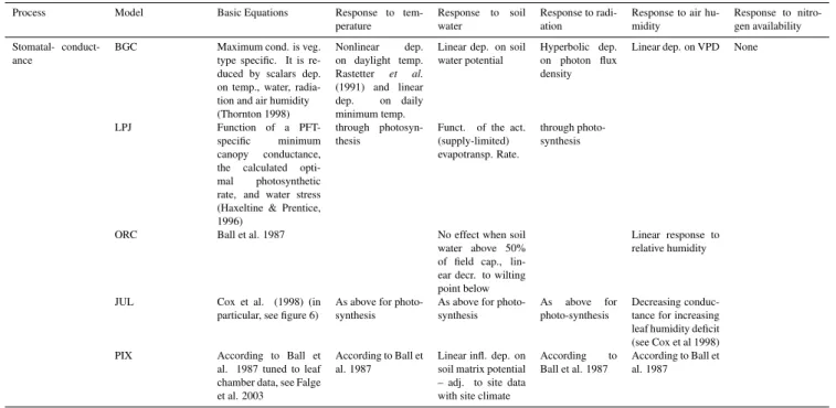
Table 1.Detailed description of the major ecosystem processes being simulated by the participating models.

Model: Biome-BGC LPJ ORCHIDEE JULES PIXGRO MOD17+ ANN

Homepage http:// www.pik-potsdam.de/lpj/ www.ipsl.jussieu.fr/

∼ssipsl/doc/doc main.html

www.jchmr.org/jules/index. html

Photosynthesis Photosynthesis of C3 and C4 plants after De Pury and Far-quhar (1997), and Woodrow and Berry (1980), dependent on leaf nitrogen content

Net Photosynthesis based on Farquhar’s model simplified by Collatz et al. (1992) + optimum canopy distribution of nitrogen (Haxeltine and Prentice, 1996) (leaf respiration is subtracted).

Farquhar et al. (1980) for C3 plants and Collatz et al. (1992) for C4 plants

Photosynthesis according to Collatz et al. (1991) for C3 and Collatz et al. (1992) C4

Net Photosyntesis according to the methodology in Owen et al. (2007) and needs input of max LAI estimated

from MODIS

(leaf respiration is subtracted)

Photosynthesis according to Reich-stein et al. (2004), empirical depen-dency of assimi-lation to climate parameters from CARBOEUROPE network Photosyntesis is simulated with Artificial Neural Network, meth-ods in (Papale and Valentini, 2003; Scardi et al., 2000), trained with 62 Carboeu-ropeIP sites Eddy covariance data treated accord-ing to Papale et al. (2006); Reich-stein et al., (2005). All networks use

a Levenberg

-Marquardt training

algorithm and

transfer functions see Reichstein et al. (2006) Stomatal

conduc-tance

Calculated as a dependence on soil water potential, minimum temperature, VPD and photon flux density according to Korner et al. (1995)

Calculated as a function of potential photosynthesis rate and water stress (Hax-eltine and Prentice, 1996)

Ball et al. (1987) based on Ball and Berry (Ball et al., 1982)

Based on Jacobs. (1994) and Cox et al. (1998, 1999), in-cluding soil-moisture depen-dence

Calculated accord-ing to Ball and Berry (Ball et al., 1982) Ecosystem respira-tion (Reco) Autotrophic respi-ration (AR) Heterotrophic res-piration (HR)

Reco: AR + HR.

AR: Sum of maintenance (MR) and growth (GR) respiration. MR: calculated separately for leaf, stem and roots, dependent on tissue nitrogen content and temperature (Ryan, 1991). GR: calculated for each plant com-partment as production costs (30% per carbon produced) HR: decomposition of litter and soil, related to chemical com-position (cellulose, lignin, hu-mus), C:N ratios, mineral ni-trogen availability, soil moisture (Andren and Paustian, 1987), Orchard and Cook (1983), and temperature (Lloyd and Taylor, 1994)

Reco: AR + HR AR: sum of maintenance (MR) and growth (GR) res-piration. MR: using fixed C:N ratios following the method in Ryan (1991) and Sprugel (1995). GR: pro-duction costs per carbon produced (25 %) HR: based on an empiri-cal Arrhenius dependence of temperature (Lloyd and Taylor, 1994). Decompos-tion depends on tissue type and moisture (Foley, 1995)

Reco: AR + HR AR: sum of maintenance (MR) and growth (GR) res-piration. MR: calculated as a function of temperature, biomass and fixed C:N ra-tios. GR: calculated for each plant compartment as production costs (28%) HR: Modified Arrhenius dependence on temperature (Lloyd and Taylor, 1994) Detailed description in (Krinner et al., 2005; Viovy, 1996)

Reco: AR + HR AR: sum of maintenance (MR) and growth (GR) res-piration. MR: stem and root dependent on temperature and mean canopy nitrogen content proportional to LAI and canopy height, leaf MR: additional moisture depen-dent (Friend, 1993). HR: soil moisture dependence according to McGuire et al. (1992)

Detailed description in Essery et al. (2003)

Ecosystem respi-ration based on Reichstein et al. (2005), decoupled from productivity and dependent on soil temperature and soil moisture

Ecosystem res-piration based on Reichstein et al. (2003b), adding short term

depen-dence on GPP,

adding Arrhenius type temperature dependence ac-cording to methods in (Reichstein et al., 2005), added quasi steady state: Reco avg=0.95xGPP over the period, Long-term mean being affected, in-ter annual variabil-ity is conserved.

Ecosystem respi-ration is estimated as the difference

between NEP,

(-NEE) and GPP, NEE being sim-ulated with the same methods as described above for GPP based on the 62 CarboeuropeIP sites.

Evapo-transpiration

Computed daily using the Penman-Monteith combination equation (Monteith, 1965)

Total evapotranspiration (Monteith, 1995)

Bulk formula to formulate surface fluxes (Ducoudre et al., 1993)

Evaporated from each soil layer by roots, and soil evao-poration dependent on soil moisture and root density (Richards, 1931) Evapotranspiration according to Reichstein (2001) and Reichstein et al. (2003b) Water balance Single bucket model:

Precipita-tion balanced with evapotransir-ation and runoff, snow-pack

Two bucket model adapted from (Neilson, 1993), precipitation balanced with runoff and drainage, snow-pack

Two bucket model with variable depth, precip-itation balanced with drainage and runoff

Multi-layer soil module based on Richards (1931), temper-ature conductivity (Cox et al., 1999), modified by snow-pack, hydrology (Gregory and Smith, 1990)

Three layer soil model, rooting depth

(50 cm short,

150 cm tall, vegeta-tion), empirical function of soil water

depletion

es-tablished from CarboEurope observation sites during the dry year 2003 Nitrogen dynamics Simulated explicit, described in

(Running and Gower, 1991; Thornton et al., 2002).

Not explicitly simulated Not explicitly simulated Not explicitly simulated Not explicitly sim-ulated

consistent with the other models in this comparison, neither cropland irrigation nor land-use change was simulated. 2.1.3 ORCHIDEE

The ORCHIDEE biosphere model describes the carbon, en-ergy and water fluxes (Krinner et al., 2005; Viovy, 1996; Ta-ble 1). ORCHIDEE differentiates between 12 different plant functional types over the globe (7 of significance over Eu-rope), similar to LPJ, of which two are representing crops

with C3 and C4-photosynthesis as fertile, harvested grass-land. Long-term vegetation dynamics, adapted from the LPJ model (Sitch et al., 2003) are not simulated here for con-sistency with other models. ORCHIDEE runs with hourly time-steps climate forcing.

2.1.4 Joint UK Land Environment Simulator (JULES) JULES is a land-surface model based on the MOSES2 land surface scheme (Essery et al., 2003) used in the Hadley

(4)

Centre climate model HadGEM (Johns et al., 2006), also incorporating the TRIFFID DGVM (Cox, 2001; Cox et al., 2000, Table 1). The model simulates carbon, water and en-ergy fluxes on 9 sub-grid tiles, including 5 plant functional types: broadleaf and needleleaf trees, C3 and C4 grasses and shrubs. In this study JULES is driven by hourly time-steps (see Tables 2 and 3). JULES does not simulate crops and crop management and represent these as natural C3 grasses. Due to technical reasons the model was run with homoge-nous soil depth of 3 m everywhere.

2.1.5 PIXGRO

PIXGRO is a canopy flux and, in the case of short-stature vegetation (grassland, crops, tundra, or wetlands), growth model for simulation of carbon and water fluxes (Adiku et al., 2006; Reichstein, 2001; Reichstein et al., 2004, Table 1). The model has been applied on landscape to continental scale and regions (Tenhunen et al., 20072; Tenhunen et al., 2007). In this continental scale study, the single-layered canopy model described in Owen et al. (2007) was applied. Canopy capac-ity for CO2uptake is estimated from CO2flux measurements

at the sites of CarboEurope network for conifer and decid-uous forests, Mediterranean shrublands, grasslands, tundra and crops. PIXGRO uses remote sensing data from MODIS to establish the max LAI for forests and shrublands of each year. Crops are represented as summer and winter grains, root crops, and maize. Phenology across the continent is based on temperature, principles related to winter dormancy and spring green up as elaborated by Zhang et al. (2004). Crops’ harvest is explicitly simulated.

2.1.6 MOD17+

MOD17+ is a semi-empirical diagnostic model (Reichstein et al., 2004, 2003b, 2005a, 2005b; Table 1) driven by re-motely sensed data. It is based on a radiation-use efficiency model (Nemani et al., 2003), which has been implemented for calculating the operational global MODIS-NPP product at 1km resolution (Running et al., 2004).

2.1.7 NETWORKANN

NETWORKANNis a diagnostic modeling approach based on

Artificial Neural Networks (ANNs) (Papale and Valentini, 2003; Table 1). ANN was trained with flux measurements covering seven different landcovers: deciduous broadleaf forest (11 sites), evergreen needleleaf forests (15 sites), ev-ergreen broadleaf forests and shrublands (6 sites), grasslands

2_{Tenhunen, J., Geyer, R., Adiku, S., Tappeiner, U., Bahn, M.,}

Dinh, N.Q., Kolcun, O., Lohila, A., Owen, K., Reichstein, M., Schmidt, M., Wang, Q., Wartinger, M., Wohlfahrt, G., and Cer-nusca, A.: Influences of landuse change on ecosystem and land-scape level carbon and water balances in mountainous terrain of the Stubai Valley, Austria, submitted to Global Planetary Change, 2007.

and wetland (18 sites), croplands (12 sites). The datasets used in the ANNs training were divided in three subsets, such as training, test and validation sets. The last one was only used to assess the ANN ability to simulate CO2flux.

3 Model inputs

The climate data were obtained with the regional climate model REMO (REgionalMOdel, Jacob and Podzun, 1997) forced with global 6-hourly NCEP (National Centers for Environmental Prediction) reanalyses (Kalnay et al., 1996) from 1948 until the current time. The major reason for choosing REMO derived climate data as driver for ecosys-tem model simulations in this study was a combination of its temporal continuity and quality (Chen et al., report). The prognostic variables are surface air pressure, temper-ature, horizontal wind components, specific humidity and cloud water. The physics scheme applied is a version of the global model ECHAM4 physics of the Max-Planck-Institute for meteorology adapted for the regional model (Koch and Feser, 2006). The model simulation was computed with ad-ditional “nudging of large scales” (von Storch et al., 2000). Thereby the simulated state is kept close to the driving state at larger scales, while allowing the model to freely generate regional-scale weather phenomena consistent with the large-scale state. A more detailed description of the multi-decadal simulation is given in Feser et al. (2001). The atmospheric hourly values were then interpolated to a regular latitude-longitude grid with a grid spacing of 0.25◦×0.25◦and ag-gregated to daily and monthly values as needed by the dif-ferent models (see Table 2, Table 3). The models used the REMO-derived climate from 1958 until 2005.

To include the effect of environmental change on the es-timates of the carbon-fluxes over Europe we used the an-nual values of the CO2 concentrations over the northern

Hemisphere. These values were based on ice core data from Etheridge (1996) and atmospheric data from Mauna Loa (Keeling and Whorf, 2005). They cover the time un-til the end of 2004. The CO2 concentration for the year

2005 was added by using the annual global trend reported by NOAA/CMDL of 2.08 ppm as an average from Jan-uary 2004–December 2005, (Table 3).

(5)

Table 2.Overview of the models participating in this study and the temporal resolution of the REMO derived climate-drivers needed. Hourly input (h), daily input (d), and monthly input (m). ORCHIDDE and JULES used different sub-daily resolutions in their simulations.

Model temperature Precipitation radiation humidity

TEMs

Biome-BGC d d d d*

LPJ m m m m

ORCHIDEE h h h h

JULES h h h h

PIXGRO h h h h

Diagnostic models

MOD17+ d d d d*

ANN d d d d*

*VPD

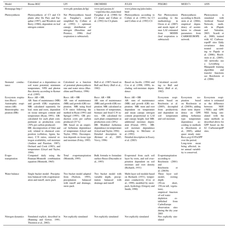
Table 3. Model input data (land surface, climate data, atmospheric CO2 concentration, atmospheric nitrogen deposition and nitrogen

fertilization) used by the terrestrial ecosystem models in this study.

Parameter Source

Albedo MODIS (MOD43B) (Lucht et al., 2000; Schaaf et al., 2002)

Elevation GTOPO 30; http://edc.usgs.gov/products/elevation/gtopo30/gtopo30.html

Soil depth TERRASTAT – Global Land Resources GIS Models and Databases, FAO Land and Water Digital Media Series # 20

Soil texture Global Soil Data Products CD-ROM (IGBP-DIS)

Landcover SYNMAP (Jung et al., 2006)

Water holding capacity pedo transfer func-tions

Cosby et al. (1984), Saxton et al. (1986)

Temperature

(max,min, daily average)

REMO Feser et al. (2001), Koch and Feser (2006),

REMO Jacob and Podzun (1997), Kalnay et al. (1997), Storch et al. (2000) Precipitation

Short wave solar downward radiation Vapor pressure deficit (VPD) Relative humidity

Atmospheric CO2concentration Etheridge (1996) Keeling and coworkers, as deposited on the ORNL CDIAC

data repository, in 2004

Atmospheric nitrogen deposition Galloway (2004), Holland (1999) Nitrogen fertilization Freibauer (2003),

http://faostat.fao.org/site/422/default.aspx

according to Freibauer (2003) and the FAO Statistics June 2006 (http://faostat.fao.org/site/422/default.aspx). We added both mineral nitrogen fertilizer as well as the total of manure and slurry from animal husbandry generating Europe-wide fertilization maps for 1961, 1989 and 2002 for the agricul-tural areas. The fertilization maps were interpolated between the years to describe the annual changes in fertilizer usage over Europe.

3.1 Model simulations

Using the same input drivers all models performed simula-tions over Europe in the domain bounded by 15◦W–60◦E and 30◦N–75◦N. This covers area from Iceland to Ural Mountains and from the Mediterranean Sea to the Barents Sea. Europe has been further divided into four regions (North, West, Central and East; Fig. 1) in order to regionally

(6)

60

30

-15

0 30

60

NORTH WEST CENTRAL EAST SOUTHEAST

Fig. 1.View of different regions of Europe: Northern Europe, West-ern Europe, Central Europe, EastWest-ern Europe.

examine the changes in terrestrial CO2exchange. This

sim-ple division to compare model output is arbitrary and does not follows ecosystem or bioclimatic zones boundaries.

The process oriented models which also calculate the car-bon pools need to spin-up to initialize slow carcar-bon and ni-trogen pools. We forced the models in a pre-industrial steady-state using atmospheric CO2 concentrations (and

ni-trogen deposition for Biome-BGC) from∼1850 (285.2 ppm, 0.0002 kgN/m2/yr) and recycling one decade of meteorolog-ical data (1958–1967) that does not exhibit significant trends of temperature and precipitation change over Europe. Af-ter establishing the slow pools, we run the models from 1850 to 1957 with transient atmospheric CO2using the same

decade of meteorological data. The last transient model runs from 1958-2005 use observed CO2concentrations and

corre-sponding meteorological data from REMO. Although rising CO2levels are responsible for long term net carbon uptake,

interannual variability in these simulations is driven solely by climate variations (Harrison et al., 2008). These final runs are the basis of our analysis.

The diagnostic models were forced with climate divers from the period 2000–2004 since they rely on remotely sensed input data from MODIS (launched in 2000). PIX-GRO was run only for 2002 and 2003, because this model is computationally very demanding.

3.2 Analysis of spatial and temporal pattern of the climate and carbon flux anomalies in 2003

Our analysis is based on carbon fluxes simulations from 1980 until 2005. We define the growing season from 1 May to 30 September. The carbon fluxes are summed over this pe-riod. The carbon flux anomalyAi,j in 2003 for each grid-cell is calculated as

Aj,i=F2003j,i− ¯F1998₋2002j,i (1)

whereF2003denotes total carbon flux over the growing

sea-son 2003,

¯

F1998−2002denotes the total carbon flux averaged over five

growing seasons (1998–2002), j and i are the longitude and

latitude respectively. In addition we estimate the change in carbon fluxes between the years 2003 and 2002, for better comparison with other studies of the carbon-flux anomaly in 2003 (Reichstein et al., 2006; Ciais et al., 2005), and for ex-plaining differences in carbon flux responses between PIX-GRO and the other models.

For each of the four European regions (Fig. 1) we es-timated the carbon flux anomaly for the growing seasons 1980–2005 weighted by area. We used the average length of a growing season from 1998 until 2002 as baseline. We have chosen the period 1998–2002 as a reference for our study be-cause we wanted to compare our results with outcomes from previous studies (Ciais et al., 2005). We use the model results from the period 1980–2005 as the quality of the climate data for this period is unbiased (Chen et al., report). In PIXGRO the calculations of carbon flux anomaly is based only on the years 2002 and 2003.

First, we estimated the anomalies of each growing sea-son (1980–2005) relative to the reference period 1998–2002. Based on these anomalies we then derived the mean anomaly for the growing seasons 1980–2005, as well as the stan-dard deviations, and the median. As the anomalies in car-bon fluxes simulated by the models varied in magnitude, we normalized the anomalies by dividing them with the corre-sponding standard deviations. This normalization procedure forced the standard deviation of the carbon flux anomaly of each model to be one.

The climate anomalies were derived similar to the carbon flux anomalies described above. The climate anomalies in-cluded growing season averages for temperature, radiation, vapor pressure deficit (VPD) and water balance. For the pre-cipitation the growing season sums were estimated.

In addition to the growing season anomalies we also de-rived the annual values of the estimated carbon fluxes and the corresponding annual anomalies.

4 Results and discussion

4.1 Regional climate and carbon flux anomalies of the growing season 2003

(7)

M.

V

etter

et

al.:

European

2003

carbon

flux

anomaly

using

7

models

567

Table 4.Regional estimated carbon fluxes of the growing season (May–September) [Tg C] for long-term mean (LT), baseline period 1998– 2002 (BL) as well as the years 2002 and 2003 with corresponding anomalies relative to long-term mean (LT), baseline (BL), and the year 2002, respectively. The models MOD17+ and ANN estimated long-term mean for the years 2000–2004 and baseline for the years 2000– 2002. Bold numbers denotes a negative anomaly; hence the value of the year 2003 is smaller than the value of the respective reference period.

NEP [Tg C] GPP [Tg C] Reco [Tg C] Climate

B L O J M A P B L O J M A P B L O J M A P T [◦_C] _{P [mm]} _{VPD [pa]} _{R [Wm}−2_]

North

LT 314 276 337 86 1038 1211 1336 656 724 936 998 570 10.9 409 456 158 L 330 276 366 85 326 286 1074 1251 1404 658 926 951 745 974 1038 573 600 665 10.9 417 429 155 2002 382 395 491 98 382 316 156 1197 1392 1569 716 995 1007 976 815 997 1078 618 612 691 820 12.0 375 522 166 2003 339 300 340 88 339 284 98 1140 1304 1426 696 946 968 896 801 1004 1085 609 607 683 798 11.6 428 477 160

2003-LT 25 24 3 2 102 93 90 41 77 68 87 39 0.7 11 48 5

2003-BL 9 24 –25 2 13 –2 65 54 22 38 20 16 56 30 48 35 7 18 –0.4 53 –45 –6 2003–2002 –43 –9 –151 –10 –43 –32 -57 –57 –88 –143 –19 –49 –39 -80 –14 7 8 –9 –6 –7 –22 0.7 20 21 2

West

LT 271 132 31 107 1019 1113 930 1571 748 981 899 1464 19.1 251 1493 230 BL 322 170 61 116 356 386 1130 1240 1005 1616 1425 1281 809 1070 944 1500 1070 895 19.1 271 1447 228 2002 353 181 82 113 364 359 399 1171 1290 1052 1644 1435 1276 1276 818 1109 969 1531 1071 917 877 18.7 293 1381 224 2003 229 –25 –99 53 262 357 162 1081 915 822 1613 1290 1173 1031 852 940 921 1560 1028 816 869 21.1 198 1838 238 2003-LT –42 –158 –130 –54 62 –198 –108 42 104 –40 22 96 2.0 –53 344 8 2003-BL –92 –196 –160 –63 –94 –29 –49 –326 –184 –3 –136 –107 43 –130 –23 60 –42 –79 2.0 –74 391 11 2003–2002 –124 –207 –181 –60 –102 –2 –90 –375 –230 –31 –145 –103 –245 34 –169 –48 29 –44 –101 –7 2.4 –95 457 15

Central

LT 505 300 170 126 1702 1468 1488 2106 1197 1168 1318 1979 18.5 305 1345 218 BL 535 284 135 101 510 490 1789 1495 1495 2163 1879 1628 1254 1210 1360 2061 1369 1138 18.9 314 1399 219 2002 559 231 77 95 584 496 156 1857 1392 1463 2301 2018 1662 1499 1298 1207 1386 2206 1434 1166 1147 19.7 326 1469 222 2003 473 215 41 134 523 508 98 1704 1304 1334 2195 1897 1565 1277 1231 1073 1293 2061 1374 1057 1072 19.9 260 1578 230

2003-LT –32 24 –129 7 2 –181 –154 89 34 –96 –25 81 1.4 –45 233 12

2003-BL –62 24 –94 33 13 18 –85 –207 –161 32 19 -63 –23 –138 –67 –1 5 –81 0.9 –54 179 11 2003–2002 –86 –9 –36 39 –61 –13 –147 –153 –151 –129 –106 –121 –96 –222 –67 –135 –94 –145 –60 –109 –75 0.2 –66 109 8

East

LT 578 382 510 129 2101 1860 2290 1818 748 981 899 1689 1055 870 14.8 359 807 187 BL 559 333 447 111 578 386 2084 1763 2192 1823 1784 1895 809 1070 944 1712 1070 895 14.9 337 890 189 2002 526 328 386 133 540 359 –28 2005 1531 2022 1818 1688 1718 1276 818 1109 969 1685 1071 917 877 15.1 263 1045 194 2003 552 345 454 154 585 357 3 2062 1872 2265 1855 1817 1905 1031 852 940 921 1700 1028 816 869 15.1 350 806 189

2003-LT –26 –37 –56 25 -38 11 -24 36 104 –40 22 11 0.3 -9 –1 1

2003-BL –7 11 7 43 7 –29 –22 108 74 32 33 10 43 –130 –23 –11 –42 –79 0.2 13 –84 0 2003–2002 26 16 68 21 45 -2 31 -58 341 244 37 129 187 –245 34 –169 –48 16 –44 –101 –7 0.0 87 –239 –5

B: Biome-BGC; L: LPJ; O: ORCHIDEE; J: JULES; M: MOD17+; A: ANN; P: PIXGR

www

.biogeosciences.net/5/561/

2008/

Biogeosciences,

5,

561–

583,

(8)

-2.5 -2 -1.5 -1 -0.5 0 0.5 1 1.5 2

GPP

-2.5 -2 -1.5 -1 -0.5 0 0.5 1 1.5 2

NEP

-2.5 -2 -1.5 -1 -0.5 0 0.5 1 1.5 2

Reco

-2.5 -2 -1.5 -1 -0.5 0 0.5 1 1.5 2 2.5 3

3.5 North West Central East

T P V R T P V R T P V R T P V R

B L O J M* _A* _{B L O J M*A* B L O J M*A* B L O J M* A*}

2003 2002 a)

b)

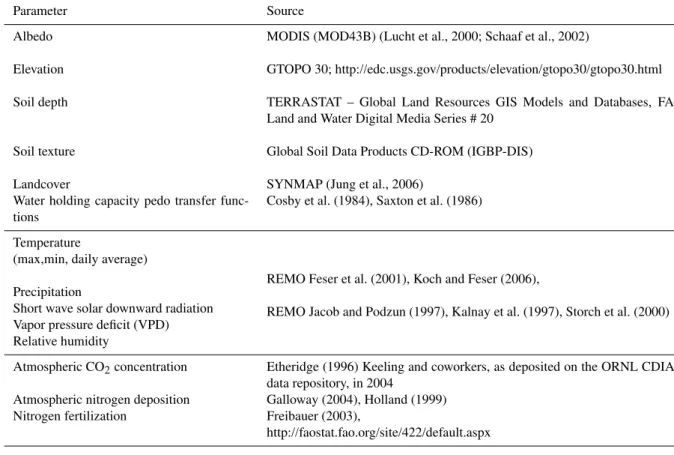
Climate

Fig. 2.Standardized area weighted(a)climate anomalies relative to baseline. T-temperature, P-Precipitation, V-Vapor pressure deficit, R-Radiation. (b)carbon flux anomalies relative to baseline. Cli-mate and carbon anomalies are aggregated over four regions of Eu-rope and values are dimension less. B-Biome-BGC; L-LPJ; O- OR-CHIDEE; J-JULES; M-MOD17+; A-ANN, Grey dots: anomaly in 2003 relative to baseline 1998–2002. Black triangles: anomaly in 2002 relative to baseline 1998–2002. White boxes: average value greater than median. Black boxes: average values less than median. * baseline: 2000–2002.

4.1.1 Northern Europe

The 2003 growing season in this region was rather warm and wet relative to the baseline and long-term (1980–2005) means. The growing season 2002 was even warmer (Fig. 2a, Table 4). All models agreed that GPP increased in both 2003 and 2002. The increase in 2002 was larger relative to both the baseline as well as the long-term mean (Fig. 2b, upper panel, Table 4). The GPP anomaly 2003 was outside the 1σ bound for Biome-BGC, LPJ, ORCHIDEE and JULES whereas the data-oriented models showed an increase too, but not as significant. This is mainly due to the increased

a)

b)

c) [°C]

[mm]

Fig. 3. The spatial pattern of the temperature and water balance anomalies through the growing season 2003 over Europe relative to baseline (1998–2002). (a)Combined spatial pattern: red areas show heat and drought, green areas show cold and wet anomaly.(b)

Temperature anomaly 2003: blue areas show a temperature increase relative to baseline, red areas a decrease.(c)Water-balance anomaly 2003: blue areas: increase in water-balance relative to baseline, red areas: decrease.

temperature in this area (∼0.7◦_{C) relative to the baseline} pe-riod of time (Table 4). This is in agreement with Churkina and Running (1998) who showed that the vegetation in the northern latitudes is temperature limited. Northern Europe is dominated by natural vegetation, mainly forests (conifer-ous and decidu(conifer-ous), which may also explain why the models showed good agreement in this region.

(9)

M. Vetter et al.: European 2003 carbon flux anomaly using 7 models 569 even more pronounced, except for LPJ and ORCHIDEE.

This is mainly explained by the increased temperature in both 2003 and 2002 (Fig. 2b, Table 4). Biome-BGC, LPJ, OR-CHIDEE and JULES showed that the Reco anomaly 2003 was outside of the 1σ bound whereas it was still inside the 1σ bound for MOD17+ and ANN. Biome-BGC and PIX-GRO estimated the smallest total Reco in the growing sea-son 2003 and JULES the largest Reco among the process oriented models. The estimated Reco over the growing sea-son 2003 as estimated by the diagnostic models (MOD17+, ANN) was smaller, but they agree with the majority of mod-els with respect to the sign of the Reco anomaly. The reason for this behavior may be due to the fact that GPP and Reco are calculated independently in the data-oriented models, so that the link between GPP and Reco is not so strong.

The resulting standardized NEP anomaly 2003 in North-ern Europe was within the range of 1σ variance for any of the models, being close to baseline, whereas the NEP anomaly 2002 clearly indicates enhanced land carbon up-take. All models except ORCHIDEE agreed in an increased NEP in 2003 relative to baseline. In this region, the increase in temperature and radiation seem to force the increase in NEP due to enhanced photosynthesis (Churkina and Run-ning, 1998) (Fig. 2b and Table 4). All models agreed that the NEP anomaly in 2003 relative to 2002 showed a decrease (Table 4). The range of the NEP over the growing season 2003 did not differ much among the models.

4.1.2 Western Europe

In 2003 this region experienced two extreme heat waves in late June and late July, and a pronounced long duration drought since the spring. The temperature increased by more than two degrees Celsius during the growing season 2003. This event was accompanied by an increase in radiation and VPD and decrease in precipitation (Fig. 2a, Table 4). Dur-ing the heat waves, the temperature anomalies reached higher values, up to 10◦C during a week (Fink et al., 2004). In 2003 all models showed a reduction in GPP. On the other hand all models agreed that GPP increased in 2002 (Fig. 2b, Table 4). The year 2002 was warm, but wetter in this region which is normally water limited. Increased precipitation leads to in-creased productivity. LPJ, ORCHIDEE, MOD17+ and ANN estimated the largest GPP anomaly 2003 being outside the lower 1σ bound. Biome-BGC and JULES also showed a re-duction of in GPP 2003 relative to baseline (Table 4), but the reduction was not significant (inside the 1σ bound, Fig. 2b). The estimated reduction in GPP in 2003 is in agreement with other studies (Reichstein et al., 2006; Schindler et al., 2006; Ciais et al., 2005). Relative to the growing season 2002, the GPP anomaly over the growing season 2003 was even stronger (Table 4).

Biome-BGC and JULES estimated an increase in Reco in 2003 relative to baseline. Reco anomaly simulated by these two models was outside of the 1σ bound (Fig. 2b, Table 4),

whereas the LPJ and ORCHIDEE estimated a decrease in Reco relative to baseline still being inside the 1σ bound. PIXGRO estimated almost no difference in Reco between 2003 and 2002 (Table 4). The sensitivity of the Reco with to respect to 2003 climate conditions seems less pronounced in Biome-BGC and JULES compared with the other pro-cess models. Both MOD17+ and ANN estimated a reduction of Reco through the growing season 2003 relative to both baseline and 2002 (Table 4). The mayor difference to the process-oriented models are the direct description of Reco based on the abiotic input in MOD17+, whereas Reco as es-timated by ANN, is just the difference between the eses-timated NEP (-NEE) and the estimated GPP, without any explicit as-sumptions about the soil conditions. The 2002 Reco anomaly showed an increase in Reco in all models.

The resulting NEP anomaly in 2003 showed a decrease mostly outside the 1σ range, with the exception of Biome-BGC, which showed a less significant decrease in compar-ison with the other models. All models agreed on nega-tive NEP 2003 anomaly relanega-tive to long-term mean, base-line and 2002 as shown in Table 4. Given the very differ-ent models, all the models have been “optimized” against the measured carbon fluxes at site-level. The common re-sponse among the models reveals a high confidence in the net carbon flux responses to a particularly extreme climate anomaly in this region. This NEP anomaly is caused by the strong increase in temperature, VPD and radiation, and re-duction in precipitation (Fig. 2b, Table 4), far outside the 1σ

range for all parameters. The growing season 2003 experi-enced a severe heat period and corresponding soil moisture deficit whereas the growing season 2002 did not show large deviations from baseline with a corresponding NEP anomaly 2002 being closer to baseline estimated by all models. The total NEP over the growing season 2003 differed strongly be-tween the models. Biome-BGC, MOD17+, ANN and PIX-GRO estimated the total NEP over the growing season 2003 to 229 Tg, 262 Tg, 357 Tg and 162 Tg respectively (Table 4). LPJ, ORCHIDEE and JULES estimated NEP values of the growing season 2003 close to neutral, the two first even es-timated a negative NEP in 2003, –25 Tg and –99 Tg respec-tively (Table 4). The large differences among the models are mainly due to the different treatment of the crop-lands (see discussion below).

4.1.3 Central Europe

In Central Europe the GPP anomaly in 2003 was less pro-nounced than in Western Europe (Fig. 2a middle panel, Ta-ble 4). This is also in agreement with the less pronounced climate anomaly in this region (Fig. 2b). Biome-BGC, LPJ, ORCHIDEE and ANN agreed in a reduction in GPP relative to baseline, the three latter also relative to the long-term mean (Table 4). The decrease was even larger relative to the grow-ing season 2002. JULES and MOD17+ showed an increase of the GPP anomaly in 2003, but agreed in a reduction of the

(10)

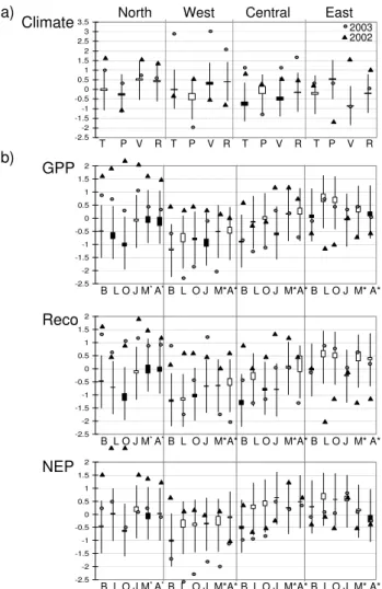
Biome-BGC

LPJ

ORCHIDEE

JULES

MOD17+

ANN

PIXGRO

[kg C m

-2

_]

(11)

Table 5.Total European carbon fluxes [Pg] and their anomalies calculated for the growing season (May–September) and the corresponding annual anomalies (in brackets). The calculated fluxes are averages over 1980–2005 (long-term mean), over 1998–2002 (baseline), and total sums for the years 2002 and 2003. Corresponding estimated anomalies are calculated relative to longterm mean, baseline and 2002 for Biome-BGC, LPJ, ORCHIDEE, JULES, MOD17+, ANN and PIXGRO. Bold numbers denote that the carbon fluxes over the growing season 2003 were smaller than over the respective reference period.

Model

Biome-BGC LPJ ORCHIDEE JULES MOD17+ ANN PIXGRO

GPP

Long-term mean 5.86 (6.44) 5.65 (7.00) 6.04 (8.28) 6.15 (7.92)

baseline 6.08 (6.71) 5.75 (7.22) 6.10 (8.56) 6.26 (8.15) 6.01 (7.60) 5.76 (7.24)

2002 6.23 (6.86) 5.65 (7.23) 6.10 (8.84) 6.48 (8.45) 6.14 (7.69) 5.66 (7.14) 5.00 (6.71)

2003 5.99 (6.57) 5.38 (6.73) 5.85 (8.01) 6.36 (8.03) 5.95 (7.30) 5.61 (6.78) 4.58 (6.09)

2003-long-term mean 0.13 (0.12) –0.27 (–0.27) –0.20 (–0.27) 0.21 (0.11)

2003-baseline –0.09 (–0.14) –0.37 (–0.49) –0.25 (–0.55) 0.10 (–0.12) –0.06 (–0.30) –0.14 (–0.46)

2003-2002 –0.24 (–0.29) –0.27 (–0.50) –0.26 (–0.83) –0.12 (–0.42) –0.19 (–0.39) –0.05 (–0.35) –0.42 (–0.62)

Reco

Long-term mean 4.19 (6.20) 4.56 (7.07) 5.00 (8.28) 5.70 (7.80)

baseline 4.33 (6.43) 4.68 (7.28) 5.09 (8.33) 5.85 (8.08) 4.24 (7.58) 3.94 (5.65)

2002 4.41 (6.49) 4.52 (7.48) 5.07 (8.36) 6.04 (8.32) 4.27 (7.55) 3.89 (5.58) 4.12 (6.25)

2003 4.39 (6.45) 4.54 (6.63) 5.11 (8.16) 5.93 (7.94) 4.24 (7.41) 3.83 (5.29) 4.11 (6.09)

2003-long-term mean 0.20 (0.25) –0.02 (–0.44) 0.12 (0.09) 0.23 (0.14)

2003-baseline 0.06 (0.02) –0.14 (–0.65) 0.02 (–0.17) 0.08 (–0.14) –0.003 (–0.17) –0.12 (–0.36)

2003-2002 –0.02 (–0.04) 0.03 (–0.85) 0.04 (–0.20) –0.11 (–0.38) –0.03 (–0.14) –0.06 (–0.29) –0.01 (–0.15)

NEP

Long-term mean 1.67 (0.23) 1.09 (–0.07) 1.05 (0.22) 0.45 (0.11)

baseline 1.74 (0.27) 1.06 (–0.06) 1.01 (0.24) 0.41 (0.07) 1.77 (0.02) 1.81 (1.59)

2002 1.82 (0.37) 1.13 (–0.25) 1.04 (0.48) 0.44 (0.12) 1.87 (0.14) 1.78 (1.56) 0.88 (0.46)

2003 1.59 (0.11) 0.83 (0.10) 0.74 (–0.15) 0.43 (0.08) 1.71 (–0.11) 1.79 (1.49) 0.47 (0.00)

2003-long-term mean –0.08 (–0.12) –0.26 (0.17) –0.31 (–0.37) –0.02 (–0.03)

2003-baseline –0.15 (–0.16) –0.23 (0.16) –0.27 (–0.38) 0.02 (0.02) –0.06 (–0.13) –0.03 (–0.10)

2003-2002 –0.23 (–0.26) –0.30 (0.35) –0.30 (–0.63) –0.01 (–0.04) –0.16 (–0.25) 0.01 (–0.07) –0.41 (–0.46)

GPP in 2003 versus 2002. Also PIXGRO estimated a strong reduction in GPP over the growing season 2003 relative to 2002.

Biome-BGC and JULES estimated an increase in Reco in 2003 relative to long-term mean (Table 4), but being close to baseline (Fig. 2b, middle panel, Table 4). ANN showed a decrease in the Reco anomaly 2003 which was outside the 1σ range (Fig. 2a, lower panel). All other models estimated the 2003 carbon flux anomaly to be inside the 1σbound. All models agreed in an increase in the Reco anomaly in 2002.

The NEP anomaly in 2003 showed mainly the same pat-tern as for Wespat-tern Europe for the models Biome-BGC, LPJ and ORCHIDEE, but the decrease in NEP was not as sig-nificant (Fig. 2b, lower panel). Also the climate anomaly over Central Europe showed the same tendency, all parame-ters showing mainly the same pattern as for Western Europe, only less significant (Fig. 2a, Table 4). JULES, MOD17+ and ANN showed a slightly increased NEP but not outside of the 1σ range (Fig. 2a, upper panel). The NEP anomaly in 2002 was slightly less prominent compared with 2003 for the mod-els LPJ, ORCHIDEE and ANN, whereas the estimated NEP anomaly 2002 showed a stronger increase for Biome-BGC, MOD17+ and ANN. JULES showed that the NEP anomaly 2002 was more decreased compared with 2003.

4.1.4 Eastern Europe

All models agreed that the GPP carbon flux anomaly in 2003 relative to baseline was small (Fig. 2b, upper panel). Biome-BGC was the only model which estimated a small decrease in GPP in 2003 (Table 4). LPJ, ORCHIDEE, JULES, MOD17+ and ANN showed an increase in GPP anomaly relative to baseline (Fig. 2b, upper panel, Table 4).

The Reco anomaly in 2003 was close to the long-term mean of the anomalies 1980–2005 (Fig. 2b, middle panel). Except Biome-BGC and JULES all models estimated an in-crease in respiration in 2003. The Reco anomaly in 2002 decreased strongly in all models (being outside of the 1σ

range), except for Biome-BGC and JULES which estimated the 2002 anomaly to be close to baseline.

The NEP anomaly in 2003 was inside the 1σ range for all models and did not differ much from the carbon flux anomaly in 2002 (Fig. 2b, Table 4). All models agreed in a positive NEP over the growing season 2003. PIXGRO estimated a NEP over the growing season 2003 close to 0. All models agreed in the sign of the NEP anomaly in Western Europe, which was also the region which experienced the strongest heat anomaly and soil water deficit as estimated by REMO.

(12)

a) GPP Reco 0.0 0.1 0.2 0.3 0.4

Jan Feb Mar Apr May JunJul Aug Sep Oct Nov Dec

Month [k g C / m ²] BGC LPJ ORC JUL MOD17 ANN 0.0 0.1 0.2 0.3 0.4

Jan Feb Mar Apr May JunJul Aug Sep Oct Nov Dec Month [k g C / m ²] BGC LPJ ORC JUL MOD17 ANN

[kg C/m²] [kg C/m²]

b) 0.0 0.1 0.2 0.3 0.4 [kg C /m²]

-200 -150 -100 -50

waterbalance [mm] gpp Reco 0.0 0.1 0.2 0.3 0.4 [kg C /m ²]

0 200 400 600 800 1.000

Soilwater [kg/m²] gpp Reco JULES Biome_BGC ORCHIDEE LPJ JULES MOD17 ANN Biome-BGC ORCHIDEE LPJ c) GPP Reco 0 0.1 0.2 0.3 0.4

Jan Feb Mar Apr May JunJul Aug Sep Oct Nov Dec

Month [k g C / m ² ] BGC LPJ ORC JUL MOD17 ANN 0 0.1 0.2 0.3 0.4

Jan Feb Mar Apr May Jun JulAug Sep Oct Nov Dec

Month [k g C / m ²] BGC LPJ ORC JUL MOD17 ANN

[kg C/m²] [kg C/m²]

d) 0.0 0.1 0.2 0.3 0.4 [kg C /m²]

0 200 400 600 800 1 000

Soilwater [kg/m2] gpp Reco 0.0 0.1 0.2 0.3 0.4 [kg C /m²]

-100 -50 0 50

waterbalance [mm] gpp Reco JULES Biome_BGC ORCHIDEE LPJ JULES ANN MOD17 Biome-BGC ORCHIDEE LPJ

Fig. 5. Seasonal average variation of GPP and Reco over the baseline period 1998–2002 for(a)crops, and(c)evergreen needleaf forests, the corresponding relationship with modeled soil water content and the water balance (estimated from precipitation, shortwave radiation and temperature) for(b)crops and(d)evergreen needleaf forests. Error bars denote averaged monthly standard deviation over the baseline period from 1998 to 2002. Due to technical reasons JULES was run with soil depth equal 3 m for all land-cover types.

5 Why do the models differ in their gross carbon flux

responses to the 2003 climate anomaly?

The reasons for the different GPP and Reco responses to the climate anomalies among different models can be summa-rized as follows:

(i) The first reason is various treatment of the crop-/cropland phenology among the models. Biome-BGC, OR-CHIDEE and JULES represent the crops with fertilized grasses, super grasses and natural grasses respectively, with no harvest. Thus, GPP is accumulated over the whole pe-riod and the grass/crop is left to senescence. This causes a larger standing biomass, which results in larger autotrophic respiration (mainly maintenance respiration) and a higher heterotrophic respiration due to larger litter and soil organic matter pools compared with models including harvest. In contrast to Biome-BGC, ORCHIDEE and JULES, LPJ and PIXGRO account for the management of the crops. In LPJ, harvest is determined through a sum over growing de-gree days (Bondeau et al., 2007) which determines maturity, thereafter the crop is harvested. In 2003 the warm tempera-tures accelerated the maturity-processes, and crops were har-vested earlier compared with not so warm periods. Hence the time for assimilating carbon was also shorter. In addition less biomass is left to senescence and cause less heterotrophic

respiration compared with the other models. PIXGRO use a simple climate zone dependence to establish the sawing and harvesting of the crops. The data-oriented models, both MOD17+ and ANN have a direct connection between the abiotic factors and GPP and have no direct coupling with the soil-processes, further the harvesting is implicit through the input data (satellite fAPAR, and measured NEE, respec-tively).

(13)

M. Vetter et al.: European 2003 carbon flux anomaly using 7 models 573 Both ORCHIDEE and JULES have a hourly resolution

(Table 2), and, hence are capable of simulating the effects of peak daytime evaporative demand on ecosystem water stress. This is especially important because the anomaly of maxi-mum daytime temperature during the heat waves was higher than the anomaly of the nighttime temperatures. This reso-lution of the diurnal cycle enables ORCHIDEE and JULES to simulate rapid increases in transpiration and decomposi-tion after a short rain event, which leads to a stronger sub-daily variation of Reco than compared to Biome-BGC (sub-daily variation) and LPJ (monthly variation). Also differences in the model simulations of evapotranspiration occur due to the differences in soil structure. JULES utilizes a four layer soil module where the decomposition of soil organic carbon is only sensitive to soil humidity and temperature in the upper 10 cm. Depending on the root distribution, the decompo-sition and water availability is more or less drought sensi-tive. PIXGRO has also a high temporal resolution, but the productivity is decoupled from the soil processes (Table 1). PIXGRO estimated almost no change on Reco between 2003 and 2002.

Furthermore, vegetation feedbacks on soil moisture play an important role in understanding the variations in GPP and Reco. Biome-BGC estimates canopy conductance as a direct function of atmospheric VPD, soil-water potential and min-imum temperature. In 2003 VPD was regionally extremely high, and therefore simulated stomatal conductance and tran-spiration in Biome-BGC were strongly reduced. Higher plant available water causes in Biome-BGC the microbial activ-ity to increase, enhancing the decomposition of soil organic matter. This may lead to increased soil mineral N, which in turn increases GPP also under water stressed conditions hence reducing the drought reduction in GPP compared with the other models (LPJ, ORCHIDEE, JULES and PIXGRO). JULES estimates an even less reduction in GPP, which shows that this model seems to be less sensitive to drought stress, a direct impact of the differentiated soil water distribution and the below-ground biomass distribution (Table 1).

(iii) The sensitivity of carbon fluxes to drought varies from model to model and can be directly related to the different modeling approaches. Models which simulate crop or grass harvest seem to have higher drought sensitivity than mod-els without harvest which may be due to increased bare-soil evaporation. Also the sensitivity to drought is higher in the models utilizing a two layer soil hydrology model. JULES has a very detailed soil hydrology and seems to be the least drought sensitive model used in this study. It has yet to be determined whether the different model sensitivities to drought are due to the carbon components sensitivity to soil moisture, or different hydrology schemes simulating differ-ent soil drying under the same climate forcings. Guo and Dirmeyer (2006) showed that many hydrology models sim-ulate interannual variability of soil moisture better than the absolute values. However, the carbon flux sensitivity to dry-ing will depend on the baseline level as well as the anomaly.

Hence, our findings illustrate the need of further model de-velopment and model evaluation against site-level measure-ments and inventories, including soil moisture observations where available, which may reduce the model differences and increase the reliability of the model estimated European carbon balance in the future.

5.1 Spatial patterns of the climate and carbon flux anoma-lies in 2003

In 2003 the climate anomaly over Europe showed across all the models a typical dipole pattern (Fig. 3). Western and Central Europe were exposed to a strong heat and drought anomaly, which was more prominent in western parts than in the central region. Eastern Europe exhibited a cold and wet anomaly. The region between these major anomalies exhib-ited intermediate conditions. This climate anomaly pattern was also seen in the spatial NEP anomaly in 2003 (Fig. 4).

In 2003, the NEP decreased over large areas of Europe (Fig. 4, areas in red color), showing a clear dipole pat-tern. These affected areas correspond directly to the climate anomalies over the same time period (Fig. 3). LPJ, OR-CHIDEE and PIXGRO estimated greater affected areas (5.18 106, 5.42 106 and 5.64 106km2 respectively) than JULES, Biome-BGC, MOD17+ and ANN (4.19 106, 4.76 106, 3.93 106 and 3.37 106km2 respectively). The three latter mod-els estimated a more heterogeneous pattern over Western and Central Europe. Models agreed well in the spatial pattern of vegetation responses to the cold and wet anomaly. There is an area with increased carbon sequestration (blue colors) be-tween the dry and warm area, and the cold and wet area. MOD17+, ANN and JULES show the greatest extent of this area in Eastern Europe. All models agreed that the 2003 NEP anomaly was positive over Scandinavia and North Eastern Russia. The spatial pattern of 2003 anomaly estimated by PIXGRO differs relative to the other models especially for Northern and North Eastern Europe as the growing season 2002 is used for the anomaly estimate. As shown earlier, the growing season 2002 was exceptionally warm in com-parison with both 2003 and baseline for this area (Fig. 2a, Table 4). This caused an increased productivity in 2002 rela-tive to 2003. Nevertheless, the good agreement in the spatial pattern of the net ecosystem productivity anomaly in 2003 among models of different complexity and structure sugest a good confidence in this pattern. However, the differences in gross fluxes across the models, suggests that much work remains to be done to quantify the response of ecosystem C fluxes to climate. Reichstein et al. (2006) showed that on a transect through Europe most site-measurements of NEP showed a negative averaged monthly NEP anomaly (July-September) as the difference between 2003 and 2002. In Germany, southern upper Rhine plain, the measured NEE in August and September 2003 was significantly lower than in 2004 (Schindler et al., 2006). Jolly et al. (2005) also showed

(14)

that the heat wave in 2003 caused an increased productivity in the Alps, which could also be seen in all models.

5.2 Contribution of the European carbon flux anomaly to the atmosphere in 2003

The length of the period chosen as reference influences the prominence of the anomalous event. In most models the prominence of 2003 anomaly declined with lengthening of the reference period from one year to 16 years (Table 4, Ta-ble 5). The 2003 anomaly for annual net carbon fluxes ranged between 0.35 and –0.63 Pg C for a reference period of one year and between 0.17 and –0.37 Pg C for a reference period of 16 years for the whole Europe.

Independent of the reference period (long-term mean, baseline or 2002) all models agreed on an anomalous carbon release from the European ecosystems to the atmosphere in 2003 (Table 5). Over the growing season 2003 the European ecosystems emitted between 0.002–0.27 Pg of carbon to the atmosphere. Using the baseline period (1998–2002) Ciais et al. (2005) estimated the anomaly of the summer 2003 (July– September) for Europe to be –0.5 Pg using ORCHIDEE (with a different forcing than in this study). This value is larger than the maximum value in our study (–0.27 Pg, OR-CHIDEE) which can be related to different definitions of the growing season in these two studies (May–September in this study, relative to July–September in Cias et al., 2005). The growing season 2002 was obviously not an average year, be-ing wetter and more productive than the long-term mean and the baseline for most of the models. Using this year to es-timate the carbon flux anomaly of the growing season 2003, would lead to a high estimate of the anomalous flux ranging between 0.01 and 0.41 Pg. The additional carbon flux from land to the atmosphere resulted from a reduced gross primary productivity which reduction was between –0.37 Pg and – 0.06 Pg relative to baseline over whole Europe. One model (JULES) estimated an increase in gross primary productivity of 0.19 Pg over the growing season 2003. All models agreed on a reduction of GPP in the growing season 2003 relative to 2002. Biome-BGC, ORCHIDEE and JULES estimated an overall increase in ecosystem respiration in 2003 relative to baseline of 0.06, 0.02 and 0.12 Pg, respectively. The other models LPJ, MOD17+ and ANN, indicated a total decrease of ecosystem respiration over the growing season 2003 of – 0.14, –0.003 and –0.12 Pg relative to baseline, respectively.

All models except ANN showed that the effect of 2003 drought on the annual carbon budget was lower than on the carbon budget of the growing season. Most likely is this a result of a diversity of vegetation types across Europe.

In Fig. 5 we have plotted the average seasonal variation of the GPP and Reco over the baseline period of the models respectively, as well as the averaged monthly values of GPP and Reco in dependence of soil-water and water-balance. We selected two 1 by 1 degree areas which were dominated by crop and conifers respectively. In each of these areas we

selected the 0.25 by 0.25 degree grid cells that contained more than 90% land cover of crop (Western Europe Car-bon anomaly: 5 grid cells) and of conifers (North Eastern European carbon anomaly: 9 grid cells), respectively. The process-models showed a clear relation in the average GPP and Reco during the baseline period with the modeled water content. Especially JULES shows a very high soil-water content for both land cover types, which may be due to the different soil-depth used in the simulations. Due to the exponential distribution of the root-depth, not all of the soil-water are available for the plants (trees reaches larger depths that grasses).

The models show a very different seasonal behavior for the crop site. LPJ and ORCHIDEE show a very early in-crease in GPP and respiration where as MOD17, ANN and especially Biome-BGC show an increase later in spring. The overall maximum of the GPP does not differ greatly amongst the models. Conversely, JULES calculated the highest Reco which may be due to a combination of the larger soil-depth and the larger soil-carbon pools. LPJ is showing two dif-ferent respiration peaks during the year associated with re-growth of grasses after harvest, whereas the other models have the highest respiration in May or June. The conifer grid cells show a much more comparable variation of GPP and Reco between the models over the year baseline period. Only the averaged maximum differs slightly which is mostly a result of the temperature sensitivity (see Jung et al., 2007). These results highlight our overall conclusion that the major differences among the models are due to their treatments of crop functioning, which is aggravated by the lack of crop spe-cific parameterization in most of the models (except LPJ) and the crop specific management. The European carbon flux in the growing season of 2003 is dominated by the ecosystems experiencing extreme drought. The annual carbon budget is, however, composed of contributions from more diverse ecosystems types and is overall less responsive to climate anomalies.

6 Conclusions

(15)

M. Vetter et al.: European 2003 carbon flux anomaly using 7 models 575 The models differ in their GPP and Reco responses to the

hot and dry anomaly in Western and Central Europe. The di-agnostic models estimated less variation in Reco compared to the process-oriented models. The links between GPP, Reco, and belowground processes should be revisited in the model structure for both, the process-oriented and the diagnostic models. A detailed data-model comparison exercise aiming to identify model abilities and uncertainties with emphasis on the response to drought is currently underway (Jung, per-sonal communication).

An interesting question to explore is how the 2003 drought influences the functioning of land ecosystems in the follow-ing years. Previous studies suggested that effect of anoma-lous climatic events could be detected in the ecosystem car-bon fluxes for at least 3–5 years after the event’s occurrence and ecosystem responses could be discontinuous (Schimel et al., 2005). Given that European ecosystems experienced drought again in 2005 the recovery of ecosystems will most likely take longer and should be investigated in the future.

(16)

Table A1. Detailed description of the process photosynthesis for the process-models Biome-BGC (BGC), Lund-Potsdam-Jena managed Land (LPJ), ORCHIDEE (ORC), JULES (JUL) and PIXGRO (PIX).

Process Model Basic Equations Response to

tempera-ture

Response to soil water

Response to radi-ation

Response to air hu-midity

Response to nitro-gen availability

Photo-synthesis BGC Maximum rate from

(De Pury and Farquhar 1997, Woodrow and Berry 1980) for shaded and unshaded canopy parts

Through

stomatal conductance

Through stom-atal

conductance

Through stom-atal conductance

Through stomatal conductance

According to rela-tionship between nitrogen demand and soil nitrogen availability

LPJ Farquhar

photosynthe-sis model (Farquhar et al., 1980, Farquhar and von Caemmerer, 1982) general. for glob. mod-elling purp. (Collatz et al., 1991, 1992). Opti-mization of the Rubisco capacacity to maxim. the daily rate of net photosynthesis (Haxel-tine & Prentice 1996)

PFT-specific tempera-ture inhibition func-tion limiting photo-synthesis at low and high temperature

Through stom-atal conductance

Colimitation by light and Rubisco activity

ORC (Farquhar et al., 80) Bowl shape func-tion,adapt. to local temp.

Tmin=-2◦_C,

Topt=25◦_C,

Tmax=38◦_C

Through stom-atal

conductance

Saturating Rubsico regener-ation rate

JUL Collatz et

al. (1991)/Collatz et al. (1992). See also Annex A of Cox (2001), and figure 7 of Cox et al. (1998)

PFT spec. function, adapt. derived from Collatz et al. (1991)/ Collatz et al (1992) to local temp., gov. by PFT spec. Tlow and Tup

Response corr. for by a soil moist. avail. factor weight. through 4 soil levels acc. to PFT spec. root depth

Saturating func-tion of incident PAR

PIX ( Farquhar et al., 1980) Enzyme

ac-tive./deactiv. (see Falge et al., 2003; Owen et al., 2007) tuned to leaf chamber data

Patchy closure reduces effective leaf area

Saturating Rubsico regener-ation rate

(17)

Table A2.Detailed description of the process stomatal conductance for the process-models Biome-BGC (BGC), Lund-Potsdam-Jena man-aged Land (LPJ), ORCHIDEE (ORC), JULES (JUL) and PIXGRO (PIX).

Process Model Basic Equations Response to

tem-perature

Response to radi-ation

Stomatal- conduct-ance

BGC Maximum cond. is veg.

type specific. It is re-duced by scalars dep. on temp., water, radia-tion and air humidity (Thornton 1998)

Nonlinear dep. on daylight temp. Rastetter et al. (1991) and linear dep. on daily minimum temp.

Linear dep. on soil water potential

Hyperbolic dep. on photon flux density

Linear dep. on VPD None

LPJ Function of a

PFT-specific minimum canopy conductance, the calculated opti-mal photosynthetic rate, and water stress (Haxeltine & Prentice, 1996)

through photosyn-thesis

Funct. of the act. (supply-limited) evapotransp. Rate.

through photo-synthesis

ORC Ball et al. 1987 No effect when soil

water above 50% of field cap., lin-ear decr. to wilting point below

Linear response to relative humidity

JUL Cox et al. (1998) (in

particular, see figure 6)

As above for photo-synthesis

Decreasing conduc-tance for increasing leaf humidity deficit (see Cox et al 1998)

PIX According to Ball et

al. 1987 tuned to leaf chamber data, see Falge et al. 2003

According to Ball et al. 1987

Linear infl. dep. on soil matrix potential – adj. to site data with site climate

According to Ball et al. 1987

(18)

Table A3. Detailed description of the process autotrophic respiration for the process-models Biome-BGC (BGC), Lund-Potsdam-Jena managed Land (LPJ), ORCHIDEE (ORC), JULES (JUL) and PIXGRO (PIX).

Process Model Basic

Equations

Response to tempera-ture

Response to radia-tion

Auto-trophic respi-ration

BGC Maintenanceresp. af-ter Ryan (1991) Growthresp. is linear dep. on mass of new plant tissue (Thorn-ton, 1998)

Q10 relationship,

Q10=2

None None None Linear dependence

on mass of nitrogen in plant tissue

LPJ Maintenance resp.:

sum of leaf, sapwood, and root respirations, based on PFT-specific respiration rates (Ryan, 1991; Sprugel, 1995)

Growth resp.: 25% of the remainder GPP -maint. resp. (Ryan, 1991)

Modified Arrhenius equation (Lloyd & Taylor, 1994), consid-ering either air or soil temperature

ORC Maintenance resp.

(Ruimy et al., 96), 30% of alloc. biomass for growth resp.

Linear response, Coefficients dep. on carbon pool. Cr(sapwood)= 1.2e-4 g/g/day Cr(leaf)= 2.3e-3 g/g/day

JUL Maintenance

respira-tion (Cox, 2001). 25% of allocated biomass for growth respiration

Linear response, Coefficients depend on carbon pool (with fixed C:N ratios). Multiple of leaf dark respiration with Q10 temperature

relationship

None, other than through moisture controls on GPP.

Canopy dark respi-ration

PIX Enzyme activation

(see Falge et al. 2003; Owen et al. 2007) tuned to leaf chamber data

Exponential increase with temperature

Not influenced Reduced with PFD above 50 µmol m−2_s−1_{to 50%}

(19)

Table A4. Detailed description of the process heterotrophic respiration for the process-models Biome-BGC (BGC), Lund-Potsdam-Jena managed Land (LPJ), ORCHIDEE (ORC), JULES (JUL) and PIXGRO (PIX).

Process Model Basic

Equations

Response to tem-perature

Response to radia-tion

Hetero-trophic res-piration

BGC Soil pool specific de-comp. rate constants corrected by scalar dep. on soil temp., moisture, and nitrogen availabil-ity (Thornton, 1998)

Exponential dep. on soil temp. after Lloyd and Taylor (1994), minimum temp. is 10◦_C

Log. dep. on soil water pot. after (Orchard and Cook, 1983; Andren and Paustian, 1987)

None None Acc. to relationship

between nitrogen demand and soil nitrogen availability

LPJ Specific decomposition rate for the labile pool (litter), and the inter-mediate & slow pools (SOM)

Modified Arrhenius rel. (Llyod & Tay-lor, 1994) cons. ei-ther air or soil temp.

Empirical soil moisture rela-tionship (Foley, 1995)

ORC Based on the

CEN-TURY model, (Parton et al. 88)

Q10 response to soil temperature temp. Q10=2

Hyperb. resp. to soil water, 1 at field cap. 0.25 at 25% of field cap.. Const. 0.25 below

JUL Cox (2001) Q10 response to

soil temp. in top 10cm (q10=2)

Piecewise linear based on McGuire et al (1992), with min. below wilt. point, and opt. mid way betw. wilt. and sat.

Ecosystem respira-tion

PIX Acc. to modified Lloyd and Taylor (1994)

Exponential incr. with temp.

Linear decr. with soil matrix pot.

None None