Modeling sugar cane yield with a process-based model from site to continental scale: uncertainties arising from model structure and parameter values

(1)

GMDD

7, 1197–1244, 2014

Modeling sugar cane yield

A. Valade et al.

Title Page

Abstract Introduction

Conclusions References

Tables Figures

◭ ◮

Back Close

Full Screen / Esc

Printer-friendly Version Interactive Discussion

Discussion

P

a

per

|

D

iscussion

P

a

per

|

Discussion

P

a

per

|

Discuss

ion

P

a

per

|

Geosci. Model Dev. Discuss., 7, 1197–1244, 2014 www.geosci-model-dev-discuss.net/7/1197/2014/ doi:10.5194/gmdd-7-1197-2014

Open Access

Geoscientiic

Model Development

Discussions

This discussion paper is/has been under review for the journal Geoscientific Model Development (GMD). Please refer to the corresponding final paper in GMD if available.

Modeling sugar cane yield with

a process-based model from site to

continental scale: uncertainties arising

from model structure and parameter

values

A. Valade1, P. Ciais1, N. Vuichard1, N. Viovy1, N. Huth2, F. Marin3, and J.-F. Martiné4

1

LSCE, CEA-CNRS, Gif-sur-Yvette, 91191, France

2

CSIRO. Ecosystem Sciences, P.O. Box 102, Toowoomba, Qld, 4350, Australia

3

University of São Paulo, Luis de Queiroz College of Agriculture, Dept Biosystems Engineering, Av. Pádua Dias 11, 13418-900, Piracicaba, SP, Brazil

4

CIRAD, UR SCA, Saint-Denis, La Réunion, 97408, France

Received: 30 December 2013 – Accepted: 14 January 2014 – Published: 31 January 2014

Correspondence to: A. Valade (aude-vaude@ipsl.jussieu.fr)

(2)

GMDD

7, 1197–1244, 2014

A. Valade et al.

Title Page

Tables Figures

◭ ◮

Back Close

Full Screen / Esc

Discussion

P

a

per

|

D

iscussion

P

a

per

|

Discussion

P

a

per

|

Discuss

ion

P

a

per

|

Abstract

Agro-Land Surface Models (agro-LSM) have been developed from the integration of specific crop processes into large-scale generic land surface models that allow calcu-lating the spatial distribution and variability of energy, water and carbon fluxes within the soil-vegetation-atmosphere continuum. When developing agro-LSM models, a

par-5

ticular attention must be given to the effects of crop phenology and management on the turbulent fluxes exchanged with the atmosphere, and the underlying water and carbon pools. A part of the uncertainty of Agro-LSM models is related to their usually large number of parameters. In this study, we quantify the parameter-values uncertainty in the simulation of sugar cane biomass production with the agro-LSM

ORCHIDEE-10

STICS, using a multi-regional approach with data from sites in Australia, La Réunion and Brazil. In ORCHIDEE-STICS, two models are chained: STICS, an agronomy model that calculates phenology and management, and ORCHIDEE, a land surface model that calculates biomass and other ecosystem variables forced by STICS’ phenology. First, the parameters that dominate the uncertainty of simulated biomass at harvest

15

date are determined through a screening of 67 different parameters of both STICS and ORCHIDEE on a multi-site basis. Secondly, the uncertainty of harvested biomass at-tributable to those most sensitive parameters is quantified and specifically attributed to either STICS (phenology, management) or to ORCHIDEE (other ecosystem variables including biomass) through distinct Monte-Carlo runs. The uncertainty on parameter

20

values is constrained using observations by calibrating the model independently at seven sites. In a third step, a sensitivity analysis is carried out by varying the most sen-sitive parameters to investigate their e_ffects at continental scale. A Monte-Carlo sam-pling method associated with the calculation of Partial Ranked Correlation Coefficients is used to quantify the sensitivity of harvested biomass to input parameters on a

con-25

(3)

GMDD

7, 1197–1244, 2014

A. Valade et al.

Title Page

Tables Figures

◭ ◮

Back Close

Full Screen / Esc

Discussion

P

a

per

|

D

iscussion

P

a

per

|

Discussion

P

a

per

|

Discuss

ion

P

a

per

|

that the 10 most sensitive parameters control phenology (maximum rate of increase of LAI) and root uptake of water and nitrogen (root profile and root growth rate, nitrogen stress threshold) in STICS, and photosynthesis (optimal temperature of photosynthe-sis, optimal carboxylation rate), radiation interception (extinction coefficient), and tran-spiration and retran-spiration (stomatal conductance, growth and maintenance retran-spiration

5

coefficients) in ORCHIDEE. We find that the optimal carboxylation rate and photosyn-thesis temperature parameters contribute most to the uncertainty in harvested biomass simulations at site scale. The spatial variation of the ranked correlation between input parameters and modeled biomass at harvest is well explained by rain and tempera-ture drivers, suggesting climate-mediated different sensitivities of modeled sugar cane

10

yield to the model parameters, for Australia and Brazil. This study reveals the spatial and temporal patterns of uncertainty variability for a highly parameterized agro-LSM and calls for more systematic uncertainty analyses of such models.

1 Introduction

In the recent years, many governments have set targets in terms of biofuels

consump-15

tion for transportation fuel (Sorda et al., 2010), resulting in a large increase in bioenergy cropping area around the world. Concerns about energy shortage, policy to reduce CO₂ emissions, and the search for new income for farmers can explain why energy policies have considered biofuels as a serious alternative to fossil fuel in many coun-tries (Demirbas, 2008). Yet, the claimed benefits of biofuels for fossil fuel substitution

20

have been questioned in terms of their net effect on atmospheric CO₂and climate, and even of their economic return (Doornbosch and Steenblik, 2008; Naylor et al., 2007). In particular, the conditions of biofuel cultivation, such as the type of crop, practice, previous land use, and local climate, have emerged as key factors that determine the effectiveness of their carbon emissions reduction (Fargione et al., 2008; Hill et al., 2006;

25

(4)

GMDD

7, 1197–1244, 2014

A. Valade et al.

Title Page

Tables Figures

◭ ◮

Back Close

Full Screen / Esc

Discussion

P

a

per

|

D

iscussion

P

a

per

|

Discussion

P

a

per

|

Discuss

ion

P

a

per

|

et al., 2008) and whose production is expected to double between 2011 and 2021 (OECD, 2012), hence the urgency to better quantify and understand regional poten-tials of bioethanol crops. Based on recent life cycle analysis studies (de Vries et al., 2010; Schubert, 2006; von Blottnitz and Curran, 2007), ethanol from sugar cane is the most competitive in terms of energy use and net carbon balance and the energy use

5

projections from the International Energy Agency foresee that by 2050, sugar cane is the only 1st generation biofuel that that will keep expanding (IEA, 2011).

The impact of sugar cane expansion on climate and carbon balance is under scrutiny with different approaches. Satellite observation data have been used to study biophys-ical effects of sugar cane expansion on local temperature in the Brazilian Cerrado

10

(Loarie et al., 2011). Survey for agricultural and industrial performances from sugar cane mills have allowed Macedo et al. (2008) to establish the carbon balance of sugar cane ethanol production in the Center-South of Brazil. Georgescu et al. (2013) simulate the hydroclimatic impacts of sugar cane expansion by forcing sugar cane land cover characteristics into a regional climate model. All approaches provide useful

informa-15

tion on impacts and potentials but are impractical to apply outside of the regions and conditions (climate, management) where they have been conducted.

In parallel with empirical approaches, significant progress has been made towards mechanistic modeling of sugar cane yields using models. Crop models are gener-ally used to simulate sugar cane production at site scale, with specific parameters

20

(Cheeroo-Nayamuth et al., 2000). Land surface models (LSM) are rather used to esti-mate the spatial distribution of crop productivity under different soil and climatic condi-tions, over a region or even over the globe but with a simpler and generic description of sugar cane plants (Black et al., 2012; Cuadra et al., 2012; Lapola et al., 2009). Agro-LSM models stand at the interface between plot-scale crop models and global Agro-LSMs.

25

(5)

GMDD

7, 1197–1244, 2014

A. Valade et al.

Title Page

Tables Figures

◭ ◮

Back Close

Full Screen / Esc

Discussion

P

a

per

|

D

iscussion

P

a

per

|

Discussion

P

a

per

|

Discuss

ion

P

a

per

|

and communicating about global models uncertainty was as well emphasized within the framework of the model inter-comparison project AgMIP – providing insights for IPCC AR5 report – in which crop models uncertainty is identified as a key theme of in-terest that was only little explored so far (Rosenzweig et al., 2013). ORCHIDEE-STICS (Gervois et al., 2004) is an agro-LSM model that has been developed from the

cou-5

pling of the agronomical model STICS (Brisson et al., 1998) and the Land Surface Model ORCHIDEE (Krinner et al., 2005), that has been applied for studies from site to continent mainly for temperate crops in Europe (Gervois et al., 2008) and has been recently adapted to sugar cane simulation (Valade et al., 2013).

Four uncertainty sources a_ffect the simulation of sugar cane biomass with

10

ORCHIDEE-STICS: (1) input uncertainty, on boundary conditions used for climate drivers and soil properties, (2) structure uncertainty, related to model equations and pa-rameterizations, (3) parameters value uncertainty, and (4) uncertainty associated with the measurements used for model evaluation or calibration. Here we focus on structure and parameters uncertainty (2) and (3) and try to estimate how these two sources of

un-15

certainties a_ffect the simulations of sugar cane harvest biomass. We want to determine which parameters are responsible for most of the uncertainty in harvest biomass sim-ulations (screening analysis) and to what extent this is related to the model’s structure (uncertainty analysis). In addition, we want to quantify this uncertainty and examine its temporal and spatial variability (sensitivity analysis).

20

In the following, we first present the sites and regions considered in this study (Sect. 2.1) and the main features of the ORCHIDEE-STICS model (Sect. 2.2). We then describe the screening algorithm used to sort the most important parameters (Sect. 2.3), and the methodology used for the uncertainty and the sensitivity analyses (Sects. 2.4 and 2.5). Then we discuss the results of the screening analysis, in terms

25

(6)

GMDD

7, 1197–1244, 2014

A. Valade et al.

Title Page

Tables Figures

◭ ◮

Back Close

Full Screen / Esc

Discussion

P

a

per

|

D

iscussion

P

a

per

|

Discussion

P

a

per

|

Discuss

ion

P

a

per

|

2 Materials and methods

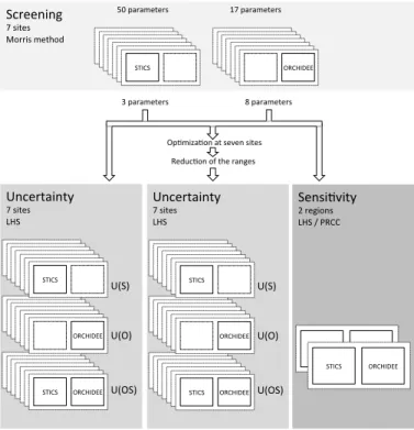
In this study, we aim to quantify the uncertainty related to the parameter values of a chain of two process-based models (STICS-ORCHIDEE) used to simulate sugar cane yield (biomass at harvest date). This is a di_fficult task because this model is a de-tailed and complex model that contains over 100 plant specific parameters within the

5

primitive equations of phenology, energy and water balance, photosynthesis and al-location. We perform the uncertainty analysis in three steps, illustrated in Fig. 1 and consisting of screening, uncertainty and sensitivity analyses, all described in more de-tails in Sect. 2. These three steps are sequential and complementary. The first step is a screening to sort the most important parameters controlling yield, and to reduce

10

the dimension of the parameter space from a large number of parameters to a few key parameters, allowing a moderate number of sensitivity simulations. The screening thus allows the restriction of the two further steps to a smaller parameter subset. The second step is an uncertainty analysis that considers all retained parameters together with their probability distributions and determines the probability distribution for the

out-15

put variable (biomass). The third step is an analysis of the sensitivity of the modeled spatial distribution of sugar cane yield to the model parameters for two large regions, in Brazil and Australia, at a spatial resolution of 0.5◦_{. The sensitivity is established from}

the spatial distribution of ranked correlations between each parameter and simulated yield in each grid point. Along the study steps, we address several problems inherent

20

to uncertainty and sensitivity evaluation such as the determination of the uncertainty on the input parameters and the spatial (regional) differences of the sensitivity of the model to its key parameters.

2.1 Sites and study areas

This study is based on sugar cane field trials in three regions (Fig. 2) where sugar

25

(7)

GMDD

7, 1197–1244, 2014

A. Valade et al.

Title Page

Tables Figures

◭ ◮

Back Close

Full Screen / Esc

Discussion

P

a

per

|

D

iscussion

P

a

per

|

Discussion

P

a

per

|

Discuss

ion

P

a

per

|

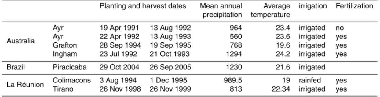
conditions and agricultural practices, as shown in Table 1, which makes them useful for our purpose to provide continental-scale sugar cane yield uncertainty estimates. More details about the four sites from Australia and La Réunion can be found respectively in Keating et al. (1999); Muchow et al. (1994); Robertson et al. (1996) and in Martiné (unpublished). The site from Brazil is described in Marin et al. (2011). The sensitivity

5

analysis of the yield spatial distribution to the model parameters is carried out for two continental-scale areas where sugar cane is cultivated at large scale. In Brazil, we consider the region encompassing partly the Sáo Paulo and Mato Grosso states, and in Australia the sugar cane cultivation belt of the northeastern coast (Fig. 2).

2.2 Model and parameters considered

10

We use the agro-Land Surface Model ORCHIDEE-STICS (Gervois et al., 2004) in a version that has been calibrated for sugar cane for Leaf Area Index at the same sites than used here (Valade et al., 2013). This model chains the crop model STICS with sugar cane specific phenology and management with the generic process-based land surface model ORCHIDEE that can be applied either at a site, or on a grid for

15

regional runs.

STICS (Brisson et al., 1998) is an agronomical model designed for site-scale op-erational applications, which describes in details the soil and crop processes associ-ated with specific crop varieties and with management practices, such as aboveground biomass, biomass nitrogen content, water and nitrogen content in the soil, yield, root

20

density. Yet, STICS is a generic crop model, because from a set of common equations it can describe a large number of crop species through specific parameterizations. Sim-ilarly, specific vectors of parameters define crop cultivars. STICS has been validated for a variety of cropping situations (Brisson et al., 2003)

ORCHIDEE (Krinner et al., 2005) is a land surface model developed for global

appli-25

(8)

GMDD

7, 1197–1244, 2014

A. Valade et al.

Title Page

Tables Figures

◭ ◮

Back Close

Full Screen / Esc

Discussion

P

a

per

|

D

iscussion

P

a

per

|

Discussion

P

a

per

|

Discuss

ion

P

a

per

|

short time scale exchanges of water and energy between the land surface and the atmosphere, as well as the processes of the carbon cycle including photosynthesis, respiration, carbon allocation, soil decomposition. The vegetation is represented in OR-CHIDEE with the Plant Functional Type (PFT) concept, by grouping species into a few categories based on the similarities of their traits and resulting in an average plant. For

5

example, sugar cane would fall in the generic “C4 crop” PFT in the standard version of ORCHIDEE, and this un-calibrated version of the model fails to reproduce site-level phenology, as shown by Valade et al. (2013).

The chaining of STICS with ORCHIDEE was performed to improve the ability of ORCHIDEE to simulate specific crops, for which the PFT concept was not appropriate,

10

as it lacks representation of crop phenology and crop management practices (Gervois et al., 2004). In the chain-like structure (Fig. 3), STICS calculates phenology, water and nitrogen requirements, and passes the key variables of Leaf Area Index (LAI), root profile and nitrogen stress as well as the input data concerning irrigation requirements to ORCHIDEE that uses them to calculate carbon assimilation and allocation, water

15

balance, and energy-related variables.

ORCHIDEE and STICS each have a large number of parameters involved at every step of a simulation over the course of a growing season. The values of these param-eters – often empirically prescribed – are not easy to measure or are not measurable at all, calling in many cases for expert judgment to set their values, when it is

imprac-20

tical to find reference values. The uncertainty of these parameters is propagated onto the output variables of ORCHIDEE-STICS and has impacts on the output variables which strength depends on the structure of both STICS and ORCHIDEE. Because of the chain-type structure of ORCHIDEE-STICS (Fig. 3), the parameters from STICS that control LAI and nitrogen stress are expected to have a weaker and more indirect

25

(9)

GMDD

7, 1197–1244, 2014

A. Valade et al.

Title Page

Tables Figures

◭ ◮

Back Close

Full Screen / Esc

Discussion

P

a

per

|

D

iscussion

P

a

per

|

Discussion

P

a

per

|

Discuss

ion

P

a

per

|

2.3 Parameter screening

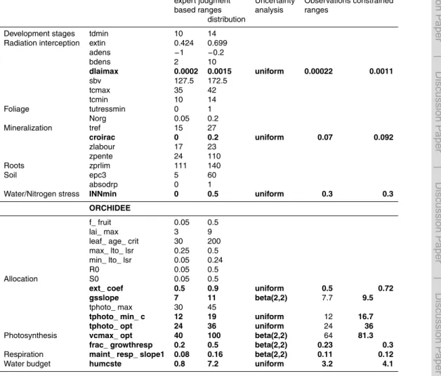
In this section, we describe the screening step that allows us to select the most in-fluential parameters upon which the model uncertainty is investigated. An initial set of 17 parameters from ORCHIDEE and 50 parameters from STICS is considered for the screening, according to their influence on the simulation of biomass production, based

5

on expert knowledge and literature as listed in Table 2. The screening analysis pro-cedure is the same as described in Valade et al. (2013). It is based upon the method of Morris (Campolongo et al., 2007; Morris, 1991; Pujol, 2009) often used to explore the parameters space for complex models with a large number of parameters. Like all screening methods, the Morris method gives qualitative information on the sensitivity

10

of the output variables to the parameters, since it only discriminates parameters based on their importance, but does not provide information on the relative difference of im-portance (Cariboni et al., 2007). Its aim is to reduce the dimensionality of the problem for further use of quantitative, computationally heavier methods (Saltelli et al., 2004).

The advantage of the Morris method is that it is computationally efficient and easy

15

to implement and interpret. It is based on a one-at-a-time approach, in which only one parameter is changed between two runs, allowing for the calculation of a local partial derivative of the output variable with respect to the input parameter, called an ele-mentary effect. The Morris method is considered to be a “global” screening method, because the algorithm is repeated several times to calculate the elementary e_ffects of

20

each parameter in several locations of the parameters space so that the average and standard deviation of all elementary effects associated with each parameter are repre-sentative of the behavior of this parameter in its whole range of variation. The results of the Morris screening algorithm can be represented by a 2-D plot of standard devi-ation vs. mean value of the elementary effects on the output variable (here harvested

25

biomass) of each parameter. A parameter with a high mean elementary e_ffect (calledµ, orµ∗_{for mean of absolute values) is interpreted as a parameter with high influence on}

(10)

GMDD

7, 1197–1244, 2014

A. Valade et al.

Title Page

Tables Figures

◭ ◮

Back Close

Full Screen / Esc

Discussion

P

a

per

|

D

iscussion

P

a

per

|

Discussion

P

a

per

|

Discuss

ion

P

a

per

|

its elementary effects (σ) is interpreted as inducing non-linearities in the model output, and/or as having interactions with other parameters.

Here, we apply the Morris method as implemented in the R “sensitivity” package (Pujol et al., 2013) using site-scale simulations of ORCHIDEE STICS across the 7 field trial sites listed in Table 1. For each site, we identify the most influential parameters for

5

the output variable harvested biomass. The parameters identified as important at least at two sites are selected for the rest of the study.

2.4 Uncertainty analysis (UA)

The goal of the UA is to quantify the overall uncertainty in the harvested biomass output variable that results from uncertain input parameter values. Firstly, based on the a

pri-10

ori probability of each parameter’s value, a Probability Density Function is assigned to each parameter in order to generate sample parameter sets according to the Latin Hy-percube Sampling (LHS) method. Secondly, an ensemble of model runs is performed using those samples. Thirdly, the uncertainty on the output variables is obtained from the statistical properties of the distribution of simulated harvested biomass from the

15

ensemble runs by defining the uncertainty as the 1-σ standard deviation of the distri-bution.

The first step is thus to generate parameters samples constrained with prior param-eters ranges and statistical distributions that are then used as inputs for ensemble simulations.

20

The parameters considered for the uncertainty (UA) for both STICS and ORCHIDEE are those selected by the screening analysis, allowing a reduction in the parameters space hypercube dimensionality and therefore in the required computing resources. Starting from the initial set of 17 and 50 parameters respectively for the screening of ORCHIDEE and STICS parameters, the Morris algorithm result (see Sect. 3.1) allows

25

(11)

GMDD

7, 1197–1244, 2014

A. Valade et al.

Title Page

Tables Figures

◭ ◮

Back Close

Full Screen / Esc

Discussion

P

a

per

|

D

iscussion

P

a

per

|

Discussion

P

a

per

|

Discuss

ion

P

a

per

|

For the UA, we use Monte-Carlo methods, which are less computationally expensive than variance-based approaches (Marino et al., 2008), making them a frequent choice in environmental sciences (Poulter et al., 2010; Verbeeck et al., 2006; Zaehle et al., 2005). The Monte-Carlo sampling scheme used here is the stratified Latin Hypercube Sampling (LHS), which is an e_fficient scheme for generation of multivariate samples

5

of statistical distributions (McKay et al., 1979). In LHS, the range of each of the k

parameters X₁, X₂, . . .X_k included in the study is divided into N intervals of equal probability. One value is randomly selected from each interval. TheN values obtained for theX₁parameter are then paired at random, without replacement, with theNvalues obtained for theX₂parameter, then to theN values obtained for theX₃parameter and

10

so on until the kth parameter. The procedure results in N sets of k parameters, or samples, that can be used for input to the model. In this study, from the 11 parameters identified by the screening,Nis set to 250 resulting in 250 simulations for exploring the uncertainty around modeled biomass for each site.

In order to get insights on the part of the uncertainty attributable to each of the two

15

models chained together, STICS and ORCHIDEE (Fig. 1), first, only the uncertainty coming from ORCHIDEE parameters is evaluated (Fig. 1), secondly, only the uncer-tainty propagated from STICS parameters (Fig. 1), and last, uncertainties propagated from both ORCHIDEE and STICS parameters are considered together through the chained model ORCHIDEE-STICS.

20

An important di_fficulty in the utilization of sampling-based UA methods is the lack of literature about a priori probability distribution of most parameters, given the depen-dency of output upon a priori assigned values (Marino et al., 2008). If most studies rely on a thorough literature search and expert judgment (Medlyn et al., 2005; Verbeeck et al., 2006; Wang et al., 2005), this approach might result in an overestimation of the

25

(12)

GMDD

7, 1197–1244, 2014

A. Valade et al.

Title Page

Tables Figures

◭ ◮

Back Close

Full Screen / Esc

Discussion

P

a

per

|

D

iscussion

P

a

per

|

Discussion

P

a

per

|

Discuss

ion

P

a

per

|

output variables outside of a given benchmark range) or by prescribing hypothesized correlations between parameters (Poulter et al., 2010; Zaehle et al., 2005). Here, after a first estimation of uncertainty based on expert opinion for the a priori parameters range (overestimation of uncertainty), we propose a second approach to overcome the scarcity of information about parameters reference distributions by reducing the

param-5

eters a priori range based on site-optimized values, thus providing narrower and more realistic a priori ranges that are constrained by observations (likely underestimation of uncertainty).

For the first a priori estimation of parameters range, ranges and distributions are assigned to parameters based on expert knowledge and previous parameterization

10

studies (Kuppel et al., 2012) and centered on their a priori values. The a priori ranges prescribed using this approach are considered as overestimations of the likely ranges for parameters’ values for sugar cane because they are adapted from studies in which parameters’ ranges were assigned for plant functional types instead of a single crop as is the case here and sometimes used for optimization studies therefore requiring wide

15

enough ranges within the model’s domain of applicability (Groenendijk et al., 2011; Kuppel et al., 2012). By using overestimated ranges for input parameters, we estimate an upper bound for the value of the uncertainty on output variables.

The second (site-constrained) a priori estimation is a refinement of the uncertainty estimation based on the idea that the “real” probability distribution of the

parame-20

ters can be approached by the distribution of optimal parameters over all the pos-sible case studies (sites, weather, management). It is of course not pospos-sible to de-termine the model’s optimal parameters for an infinite number of eco-climatic and land-management conditions, but a sample of representative case studies can provide a rough estimate of the parameters plausible range. Building on this hypothesis, the

25

(13)

GMDD

7, 1197–1244, 2014

A. Valade et al.

Title Page

Tables Figures

◭ ◮

Back Close

Full Screen / Esc

Discussion

P

a

per

|

D

iscussion

P

a

per

|

Discussion

P

a

per

|

Discuss

ion

P

a

per

|

the model data misfit as well as the parameters’ deviations from a prior knowledge. The iterative scheme is described in (Tarantola, 1987) with the hypothesis of Gaussian error on the observations and the parameters. At each site, parameter values are varied iter-atively until the best match between simulation and observation is found. More details on the calibration results can be found in the Supporting Information. We are aware

5

that the optimization of the parameters at 7 sites only to obtain a representative a priori range of the parameters distributions likely results into an optimistic estimate of this range even though the sites chosen cover di_fferent climatic, edaphic and management conditions making them well suited for applying our method.

For both a priori parameters range estimations (expert judgment vs. site

con-10

strained), when no parameter value appears to be more likely than another, a uniform a priori uncertainty distribution is prescribed. When there is some level of confidence that the a priori value is more likely, we use a beta distribution. This type of distribution is often used for uncertainty analyses, because of its adjustable shape (parameterized equation) yet having the advantage of bounded tails (Monod et al., 2006; Wyss and

15

Jorgensen, 1998). The successive analysis of both techniques provides an improve-ment in the estimation of the uncertainty from the first (expert-judgimprove-ment based, likely too pessimistic) to the second (observation-based, perhaps too optimistic) approach.

2.5 Spatial sensitivity analysis (SA)

The first step in the sensitivity analysis also consists in generating parameters samples.

20

The same parameters are considered for the SA as for the UA (Sect. 2.4), i.e. the 11 parameters (8 parameters from ORCHIDEE and 3 parameters from STICS) selected by the screening analysis.

As opposed to the UA where all parameters are considered together for their e_ffect on the distribution of the harvested biomass output variable, the goal of the sensitivity

25

analysis is to rank the influence of parameters based on their impact on the biomass and its spatial distribution obtained in the continental-scale 0.5◦_{runs. The partial}

(14)

GMDD

7, 1197–1244, 2014

A. Valade et al.

Title Page

Tables Figures

◭ ◮

Back Close

Full Screen / Esc

Discussion

P

a

per

|

D

iscussion

P

a

per

|

Discussion

P

a

per

|

Discuss

ion

P

a

per

|

a parameter after the correlation with other parameters has been eliminated (Marino et al., 2008). However, for monotonic but non-linear relationships, these measures per-form poorly and a rank transper-formation needs to be applied to the data first to linearize the relationship. The correlation calculated between the rank-transformed data is then called partial rank correlation coe_fficients (PRCC). PRCC has been found to be an

5

efficient indicator for the influence of parameters, because it is a measure of the sensi-tivity of the output to parameters (Saltelli and Marivoet, 1990) The larger the PRCC, the more important the parameter is with respect to the output variable. Here, the relation-ship between modeled biomass on a grid, and parameters is diagnosed through the calculation of the Partial Ranked Correlation Coefficients (PRCC) on each grid point

10

between the output and parameter assuming a monotonic behavior of the model. The SA is implemented from the results of the 0.7◦_{simulations over Brazil and}

Aus-tralia (see Fig. 1 and Sect. 3.5). In this regional sensitivity analysis, ORCHIDEE-STICS is run for each region on a grid of 20 by 15 grid points and 13 by 20 grid points respec-tively, driven by gridded climate forcing fields from the reanalysis products ERA-Interim

15

(Dee et al., 2011), with varying parameter values from a sampling where only bounds and no distributions were assigned to the parameters. The management information (date of planting, date of harvest, fertilization, irrigation) and the soil properties (as described in Valade et al., 2013) are assumed to be uniform across each region and were defined as typical of each area. The a priori bounds used for the parameters in

20

the SA correspond to the first version of the parameters ranges considered in the un-certainty analysis (i.e. derived from expert knowledge). As cited by Wang et al. (2005), for sensitivity analyses, Bouman (1994) advises to use parameters ranges as broad as possible within the limits of the model validity domain. Once the parameters’ a pri-ori bounds have been set, ensemble runs are performed with all the parameter sets.

25

(15)

GMDD

7, 1197–1244, 2014

A. Valade et al.

Title Page

Tables Figures

◭ ◮

Back Close

Full Screen / Esc

Discussion

P

a

per

|

D

iscussion

P

a

per

|

Discussion

P

a

per

|

Discuss

ion

P

a

per

|

The interest of carrying out such a regional sensitivity analysis is that it provides maps of the geographic patterns of the importance of each parameter, leading to a bet-ter comprehension of the mechanisms behind the paramebet-ter-related model sensitiv-ity. These results can be very useful for planning purposes, for instance to quantify what are the di_fferent factors that control sugar cane yield and ethanol production over

5

a large region under future climatic conditions as compared to present-day conditions.

3 Results and discussion

3.1 Screening

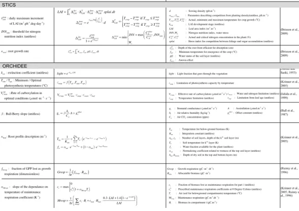
From the Morris screening method, we obtain for each parameter two indicesµ∗ _and

σ, that measure the influence of each parameter and its degree of involvement in

non-10

linearities and interactions with other parameters, respectively. Fromµ∗ _and_σ _values,

we establish a ranking of the parameters by only considering parameters involved in limited interactions and/or non-linearities (σ <2µ∗_{) and then we rank the remaining}

parameters based on theirµ∗_{index, a larger}_µ∗_{being interpreted as a more influential}

parameter. The Morris parameters ranks for ORCHIDEE and STICS are respectively

15

shown in Fig. 5a and b where each radar plot corresponds to one model. The axes refer to the parameters and the line colors to the sites. For STICS, for the sake of readability, not all of the initially selected 50 parameters are represented on the radar plot but only those parameters that pertain to the 10 top-ranked parameters at least at one site. The maximum number of 10 parameters was fixed based on examination of Morris indices

20

µ∗ _and _σ _{at individual sites that only revealed 3 to 5 sensitive parameters each time.}

The positions and roles in the model of the parameters identified as most important are shown in Fig. 3. Figure 4 gives more details, with the main equations through which these parameters affect the output variables of STICS and of ORCHIDEE.

The 3 most influential parameters of STICS (Fig. 3a) reflect the way STICS and

OR-25

(16)

GMDD

7, 1197–1244, 2014

A. Valade et al.

Title Page

Tables Figures

◭ ◮

Back Close

Full Screen / Esc

Discussion

P

a

per

|

D

iscussion

P

a

per

|

Discussion

P

a

per

|

Discuss

ion

P

a

per

|

impact of STICS parameters on harvested biomass occurs through their effect on pro-cesses related to LAI, root growth and nitrogen stress, the only STICS variables passed to ORCHIDEE for calculating biomass. This chaining of the models through three vari-ables is reflected in the identification of the 3 most important STICS parameters, which control the daily maximum rate of foliage productionδ_LAImax, the growth rate of the root

5

front, κ_root and the threshold of nitrogen nutrition index INN_min. δ_LAImax and INN_min pa-rameters are both involved in LAI calculation. Indeed, the LAI equation has four mem-bers describing four processes of the sugar cane foliage development. First, the LAI-development (∆devLAI in Fig. 4) describes the potential LAI increase through the scaling

of the daily maximum rate of foliage production by a function of the development stage

10

(k_LAI), and is logically directly controlled by the value of parameterδ_LAImax. The second member in the LAI defining equation in Fig. 4 represents the temperature effect on LAI growth through the accumulation of degrees above a temperature threshold (T_min in Fig. 3). The last two members of the equation represent processes that can limit LAI development and competition for light between plants due to planting density (_∆dens_LAI in

15

Fig. 4) and a limitation from trophic stress emerging from competition between plant components for nitrogen, based on the calculation of a nitrogen nutrition index limited by parameter INN_min. The root growth rateκ_roothas a less direct impact on LAI since it intervenes in the calculation of the root front depth, which then impacts the availability of nitrogen and water and therefore the stress status of the crop (impact onC_Nplantand

20

W_sin Fig. 4).

The 8 most influential parameters that control harvested biomass in ORCHIDEE, are identical for all sites except for the Colimaçons site (where only 7 parameters are identified as influential by the Morris method). The Morris top ranked parameters of ORCHIDEE control photosynthesis and water budget equations as well as respiration

25

(17)

GMDD

7, 1197–1244, 2014

A. Valade et al.

Title Page

Tables Figures

◭ ◮

Back Close

Full Screen / Esc

Discussion

P

a

per

|

D

iscussion

P

a

per

|

Discussion

P

a

per

|

Discuss

ion

P

a

per

|

minimum temperatures for photosynthesis. The stomatal conductanceg_sthat links as-similation and transpiration is defined by the Ball–Berry equation (Ball et al., 1987) as a function of assimilation and depends on the air relative humidity and CO₂ concentra-tion, scaled by a slope factor, called the Ball–Berry slope (β). The root profile constant (κ_hum) describes the exponential distribution of root density in the soil and is involved in

5

the definition of available water and root temperature. Finally, the extinction coefficient (k_ext) intervenes in an equation derived by Monsi and Saeki (1953), similar to Beer’s law, which describes the attenuation of light with depth in the canopy.

Two ORCHIDEE parameters controlling autotrophic respiration also stand out, with the maintenance respiration coefficient (α_Mresp) and the fraction of biomass allocated

10

to growth respiration (f_Gresp). The leafcrit_age parameter that is involved in the biomass allocation also ranked high (5th most important) but only for one site and is therefore not retained for the rest of the study.

For the chained model STICS-ORCHIDEE, the 11 most influential parameters show a good agreement between sites for the most important parameters as seen on Fig. 5

15

where ranking lines overlap for most of the parameters. Building on the results of the Morris screening analysis, we select the 8 top ranked parameters for ORCHIDEE and 3 for STICS that were revealed as influential for biomass for further uncertainty and sensitivity analysis.

3.2 Uncertainty analysis: parameters controlling biomass uncertainty at a

typi-20

cal site

In this section, we attribute the harvested biomass uncertainty to the uncertainty of the ORCHIDEE vs. STICS parameters. The simulated biomass uncertainty is a function of time during the growing season, and it differs between sites. In Fig. 6, we show the contributions of ORCHIDEE and STICS parameters respectively to the total

uncer-25

(18)

GMDD

7, 1197–1244, 2014

A. Valade et al.

Title Page

Tables Figures

◭ ◮

Back Close

Full Screen / Esc

Discussion

P

a

per

|

D

iscussion

P

a

per

|

Discussion

P

a

per

|

Discuss

ion

P

a

per

|

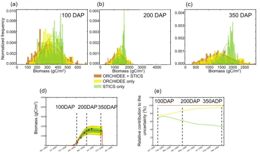
normalized frequency distributions of simulated biomass obtained from ensemble runs for three times in the growing season: (1) very early in the cycle in Fig. 6a, at 100 days after planting (DAP), (2) during the peak growing season in Fig. 6b, at 200 DAP and (3) short before harvest in Fig. 6c, at 350 DAP. We distinguish between the normalized frequency distributions of simulated biomass when considering the uncertainty

propa-5

gated from STICS parameters alone (green), ORCHIDEE parameters alone (yellow), and from ORCHIDEE and STICS parameters together (brown), along with their best-fit normal distributions overlaid. These distributions were obtained by Monte Carlo LHS ensemble runs (Sect. 2.4) with a sampling of parameters of STICS alone, ORCHIDEE alone and of both models together. We consider uncertainties starting from the time

10

when biomass reaches 50 g C m−2 _{in order to discard the emergence phase during}

which biomass is very low and uncertainties are therefore not significant.

At 100 DAP (Fig. 6a), the uncertainty distribution of biomass related to ORCHIDEE parameters U(O) spans a slightly larger range than the distribution related to STICS, U(S), and it has more extreme values. The U(O) distribution is symmetrical around the

15

mean value, with a standard deviation of 86.9 g C m−2_{. The U(S) distribution is}

non-symmetric, skewed towards larger values of biomass, and it has a slightly smaller standard deviation (76.5 g C m−2_{) than that of U(O). Combining U(O) and U(S) in}

Monte Carlo runs by varying the parameters of both models at the same time gives the total uncertainty distribution, U(O₊S), shown in brown in Fig. 6. This

distribu-20

tion has more extreme values and a higher standard deviation (112.0 g C m−2_{), i.e.}

U(O+S)>U(O)+U(S).

At 200 DAP (Fig. 6b), and later at 350 DAP (Fig. 6c), the picture has changed. First, all uncertainties distributions are wider than at 100 DAP. Secondly, the means of U(O) and U(S) are no longer in agreement, with the asymmetric U(S) distribution being even

25

(19)

GMDD

7, 1197–1244, 2014

A. Valade et al.

Title Page

Tables Figures

◭ ◮

Back Close

Full Screen / Esc

Discussion

P

a

per

|

D

iscussion

P

a

per

|

Discussion

P

a

per

|

Discuss

ion

P

a

per

|

result into increased photosynthesis and therefore biomass in ORCHIDEE. However, passed a certain threshold, the LAI impact saturates when the foliage is su_fficient for all incoming light to be captured, and therefore, uncertainty on the STICS parameters that impact LAI will not increase the uncertainty of biomass any longer. Unlike LAI, the nitrogen stress and root profile variables controlled by the parameters of STICS

5

continue to act as limiting factors on biomass throughout the peak and late growing season. The saturation of the biomass uncertainty associated with STICS parameters is stronger at 200 DAP than at 300 DAP, when biomass increase has slowed down and the role of LAI for driving biomass is less important.

On Fig. 6d, the total uncertainty U(O+S) is given for the reference simulation (with

10

parameters at their maximum likelihood values, red line) and the uncertainty on har-vested biomass can be defined as a percentage of the harhar-vested biomass in the ref-erence simulation. For the Grafton site, at harvest, the overall uncertainty is 26. %. The relative contributions of ORCHIDEE and STICS to the total uncertainty,α_O and

α_S respectively, are defined by α_O=_U(OU(O)₊_S),α_S=_U(OU(S)₊_S). The evolution of these

con-15

tributions to the total uncertainty is shown in Fig. 6e. We can see in this example that U(O)>U(S) during the entire growing season, but with a decrease of U(S), and an increase of U(O) such that the increase in biomass uncertainty seen on Fig. 6d be-comes increasingly dominated by uncertain ORCHIDEE parameters. The progressive increase in the weight of ORCHIDEE parameters uncertainties is due to the reduction

20

in the role played by LAI for biomass increase along the growing season. Indeed, if early in the season the foliage is crucial to allow photosynthesis and carbon alloca-tion, later in the cycle, other processes become important as well and passed a certain LAI for which all incoming light is captured, it might not even play a role anymore and then the STICS parameters only impact biomass accumulation through nitrogen stress

25

(20)

GMDD

7, 1197–1244, 2014

A. Valade et al.

Title Page

Tables Figures

◭ ◮

Back Close

Full Screen / Esc

Discussion

P

a

per

|

D

iscussion

P

a

per

|

Discussion

P

a

per

|

Discuss

ion

P

a

per

|

3.3 Uncertainty analysis: role of ORCHIDEE vs. STICS parameters in controlling biomass uncertainty at 7 sites

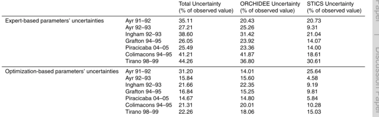
Table 3 summarizes the results of the overall parametric uncertainty analysis at the 7 sites, including Grafton. The total uncertainty U(O₊S) ranges between 25.5 % of biomass at Piracicaba, Brazil during 2004–2005 and 44.26 % of harvested biomass

5

at Tirano, La Réunion in 1998–1999 yielding an average uncertainty on biomass at harvest due to uncertain parameter values of the chained model ORCHIDEE-STICS of 34.0 % of harvested biomass across the 7 sites, in the order of previous results on different variables in similar studies using process-based models such as (Dufrêne et al., 2005) who found an uncertainty of 30 % on modeled NEE for a forest sites in

10

France with the CASTANEA model.

As for the ORCHIDEE vs. STICS relative contributions to the uncertainty of simu-lated biomass at all sites, the results at each site are not identical but display a similar general pattern shown by Fig. 7. For all sites, the ORCHIDEE parameters contribution to total uncertainty increases during the cycle, or remains approximately constant for

15

Ingham in 1992–1993, and increases during the growing cycle to dominate entirely the total uncertainty at the end of the cycle compared to STICS parameters. The STICS contribution to overall uncertainty decreases during the growing season to reach a min-imum by the end of the growing season. For sites Piracicaba during 2004–2005, Tirano in 1998–1999 and Colimaçons during 1994–95, during the beginning of the cycle the

20

U(S) is even larger than U(O). The results for Ayr in 1991–1992 display a less clear pattern. Indeed, at the end of the cycle, the contributions of ORCHIDEE and STICS to the total uncertainty are almost equal, due to an increase in STICS contribution during the second half of the cycle. This result confirms a hypothesis made in Valade et al. (2013) where the difficult calibration of LAI at this site was attributed to the

sim-25

(21)

GMDD

7, 1197–1244, 2014

A. Valade et al.

Title Page

Tables Figures

◭ ◮

Back Close

Full Screen / Esc

Discussion

P

a

per

|

D

iscussion

P

a

per

|

Discussion

P

a

per

|

Discuss

ion

P

a

per

|

3.4 Uncertainty analysis: constraining uncertainty from sites optimization

Optimizing the 11 ORCHIDEE-STICS parameters selected from the screening analy-sis at 7 sites leads to a reduction of the width of the a priori uncertainty distribution of the parameters (Table 2). Carrying out the same uncertainty analysis with a narrower uncertainty range of parameters (thanks to their site calibration) leads to an important

5

reduction of uncertainties of biomass both for the STICS and ORCHIDEE components of uncertainty. This can be seen by comparing Fig. 6 (initial range of parameters) with Fig. 8 (narrower range after parameters calibration at the sites). For site Grafton dur-ing 1994–1995 for example, U(O+S) gets reduced from 26 % to 17 % of the reference harvested biomass, U(O) from 24 % to 15 % and U(S) from 14 % to 10 %. Figure 9 and

10

Table 3 (bottom section) show the uncertainty contributions and overall uncertainty estimates for the 7 sites after observation-based reduction of the a priori uncertainty on parameters. The overall parametric uncertainty of biomass defined as the 1-sigma standard deviation of the (O₊S) distribution has thus been reduced to 21 % in aver-age, to 11.48 % when attributed to STICS alone, and to 17.15 % when attributed to

15

ORCHIDEE alone, (Table 3).

The ORCHIDEE and STICS contributions to the total uncertainty keep the same general pattern as with the initial parameters uncertainty distribution, with a domination of ORCHIDEE parameters in the uncertainty towards the end of the growing season (Fig. 9). Compared with the first uncertainty budget with expert-based parameters

un-20

certainties (Fig. 8), there is generally a slight decrease in the STICS contribution at the end of the season.

We have thus established full uncertainty budgets for the two components of the ORCHIDEE-STICS chain of models, which has revealed variations in the uncertainty in the biomass simulation from site to site. The next step is to discriminate between the

25

(22)

GMDD

7, 1197–1244, 2014

A. Valade et al.

Title Page

Tables Figures

◭ ◮

Back Close

Full Screen / Esc

Discussion

P

a

per

|

D

iscussion

P

a

per

|

Discussion

P

a

per

|

Discuss

ion

P

a

per

|

3.5 Spatial sensitivity analysis: sensitivity of sugar cane yields to the model parameters for Brazil and Australia

The overall parametric uncertainties have been quantified at 7 sites and attributed to either STICS or ORCHIDEE. The sensitivity analysis (SA) in this section will go a step further and leads to discriminate the di_fferent parameters that contribute to the spatial

5

distribution of uncertainty over the two regions considered. This sensitivity analysis is performed at regional scale because from the previous section, we have seen that the uncertainty in the biomass simulation varies from site to site.

Ensemble runs at regional scale were realized over Brazil and Australia each with dif-ferent value combinations for the 11 parameters previously selected through the Morris

10

screening analysis (Table 1). The Partial Rank Correlation Coe_fficients (PRCC) were then calculated for each pixel in each of the two regions (see Sect. 2.5), and the SA results are discussed for two dates during the growing season, 200 and 350 days after planting (DAP). The SA results express the strength of the relationship between an uncertain parameter and the simulated biomass at harvest at each pixel. The

statisti-15

cal significance of the PRCC calculated for each grid cell is tested with the associated

pvalues, and non-significant PRCC are removed (pvalue<0.05). The first date 100 DAP examined for site scale UA studies (Sect. 2.3) is not shown here, because no statistical significance was found in the correlations between the parameters and the harvested biomass at 100 DAP. Then, the pixels statistically significant PRCC

calcu-20

lated for each parameter can be analyzed both in a geographical projection (latitude, longitude) (Figs. 11 and 12, columns 1–2 and 4–5) and in a (Temperature, Precipitation) climatic space projection (Figs. 11 and 12, columns 3 and 6). The regional sensitivity analysis thus carried out for sugar cane growing areas in Brazil and Australia shows the magnitude, spatial distribution and climatic dependency of the sensitivity of

har-25

(23)

GMDD

7, 1197–1244, 2014

A. Valade et al.

Title Page

Tables Figures

◭ ◮

Back Close

Full Screen / Esc

Discussion

P

a

per

|

D

iscussion

P

a

per

|

Discussion

P

a

per

|

Discuss

ion

P

a

per

|

Across both regions in Brazil and Australia, we find that the sensitivity of biomass to the model parameters is not uniformly distributed. This means that the simulated yield depends on different parameters within different parts of the same region. This result shows that applying a model at one site to determine the most important param-eters, and generalizing its conclusion across a region generates biased conclusions.

5

Considering only the first most important parameter in each pixel (Fig. 10), we can see that early in the cycle (200 DAP, Fig. 10a) four parameters dominate the spatial distribution of the U(O₊S) uncertainty of biomass at 200 DAP, both over Brazil and Australia. These parameters are three ORCHIDEE parameters involved in the pho-tosynthesis process, the minimum and optimum temperature for phopho-tosynthesisT_min,

10

T_opt, and the maximum rate of carboxylation V_Cmaxopt , and one parameter from STICS

δ_LAImax, defining the maximum rate of increase of LAI and only appearing in the Aus-tralian region. In Brazil, the parameterV_Cmaxopt is the first most important parameter for 93 % of the area, whereas the optimum and minimum photosynthesis temperatures parameters only dominate in respectively 3 and 4 % of the area. In Australia, the

pa-15

rameters’ domination is more balanced with 37.5 % for each of V_Cmaxopt and δ_LAImax and 25 % forT_min.

Later in the growing season (350 DAP, Fig. 10b), consistently with the results of the site-scale uncertainty analysis, the influence of the STICS parameters decreases until no STICS parameters appear any longer as a dominant parameter in any of the

20

regions. At this later stage in the season, two parameters stand out as explaining most of the uncertainty in most pixels of both regions,V_Cmaxopt and T_min. In Brazil,V_Cmaxopt is still the most sensitive parameter for most of the region, butT_optdisappeared and the area dominated byT_min expanded and now covers the cooler area of the southeast coastal zone. In Australia, the area dominated byV_Cmaxopt expanded into most of the region and

25

(24)

GMDD

7, 1197–1244, 2014

A. Valade et al.

Title Page

Tables Figures

◭ ◮

Back Close

Full Screen / Esc

Discussion

P

a

per

|

D

iscussion

P

a

per

|

Discussion

P

a

per

|

Discuss

ion

P

a

per

|

Figures 11 and 12 focus on the values of the PRCC for each parameter as well as their spatial distribution. Their projection in a Temperature-Precipitation space for a given time (Fig. 11 for 200 DAP, Fig. 12 for 350 DAP) give more insights on the dependency of the sensitivity to the climatic conditions along the growing cycle. As an example, the sensitivity of the simulated biomass toT_opt is highly sensitive to the

5

average temperature of the location. At low-temperature sites, where temperature is a limiting factor for crop growth (below 17◦_{C), the PRCC is higher than 0.8, whereas at}

high-temperature sites (above 22◦_{C) the PRCC is below 0.3. Sites with temperatures}

above 25◦_{C do not even show significant correlations (grey symbols on the scatter}

plot).

10

For the parameterκ_hum, which describes the root profile of the cane (inverse of root depth), the dependency is most obvious on precipitation amount. For annual precipita-tions above 2500 mm, no significant correlation is found.

Comparing the regional sensitivities at two times in the growing season shows again the decrease in the importance of STICS parameters whereas all of most important

15

ORCHIDEE parameters have larger RPCC than earlier in the season.

4 Concluding remarks

In the perspective of applying spatially explicit mechanistic vegetation models such as ORCHIDEE-STICS to biofuel yield simulations we have sought the quantification and understanding of parametric uncertainty propagation in the model, both at site

20

level and at continental scale over two large regions, Australia and Brazil. For this, a rigorous analysis of the uncertainty budget of simulated sugar cane biomass has been established, using a step by step tracking of uncertainty in the model.

The main parameters from the two chain components of the model responsible for most of the uncertainty propagation have been identified through a Morris screening

25

(25)

GMDD

7, 1197–1244, 2014

A. Valade et al.

Title Page

Tables Figures

◭ ◮

Back Close

Full Screen / Esc

Discussion

P

a

per

|

D

iscussion

P

a

per

|

Discussion

P

a

per

|

Discuss

ion

P

a

per

|

the root profile constantκ_hum, the parameters for respiration, slope of the Ball–Berry relation β, maintenance and growth respiration parameters f_Gresp and α_Mresp for the ORCHIDEE carbon, water and energy model. For the STICS model, the most influen-tial parameters are those responsible for simulation of phenology, nitrogen and water stress, the parameters describing the maximum rate of carboxylation, the maximum

5

growth rate of the root front and the threshold for nitrogen stress have been found to have the greatest role.

We used two approaches for estimating the total uncertainty propagated from the pa-rameters into the model by assigning uncertainties on papa-rameters with two methods, one “pessimistic”, in which a priori parameter uncertainty bounds are set based on

10

expert judgment, and one optimistic where smaller uncertainty are derived by an opti-mization of the model parameters at several sites and this providing a smaller arguably more realistic a priori uncertainty range.

We found that all these parameters together contribute to an overall uncertainty of 21 % on sugar cane biomass simulations with an agro-LSM model and that this amount

15

is variable among sites with different climatic, edaphic and management situations. We also analyzed this uncertainty separately for each component of the model and found that whatever estimate chosen for the parameters uncertainty, by the end of the growing season, the uncertainty propagated from the phenology module STICS decreases and the overall uncertainty is almost totally explained by the ORCHIDEE uncertainty.

20

The overall origin of uncertainty has then been diagnosed in even more detail through a regional sensitivity analysis allowing the identification of the parameter for which harvested biomass is most sensitive for each pixel within regions of Australia and Brazil. We revealed a strong heterogeneity of the results based on climatic conditions and also variability in time that confirms the results of the uncertainty analysis, by showing

25

(26)

GMDD

7, 1197–1244, 2014

A. Valade et al.

Title Page

Tables Figures

◭ ◮

Back Close

Full Screen / Esc

Discussion

P

a

per

|

D

iscussion

P

a

per

|

Discussion

P

a

per

|

Discuss

ion

P

a

per

|

models such as agro-LSM, especially when applying these models to answer questions related to political decisions such as biofuels burning topics.

As an example, combining our optimistic uncertainty estimation with the results from (Lapola et al., 2009) for irrigated sugar cane (obtained with the model LPJml, very sim-ilar to ORCHIDEE-STICS), we can evaluate the range assorted with their estimation

5

of land requirements to fulfill the demand in ethanol in Brazil. They found a mean yield of 74.36 t ha−1_{, and conclude that to fulfill government targets, the sugar cane areas}

would need to expand by 2.8 million hectares. With the hypothesis that our uncertainty calculation is applicable to the LPJml results, we can translate the potential mean pro-duction uncertainty as a range of (59–90 t ha−1_{). The land requirements when including}

10

parameters uncertainty would then becomes (2.3–4 million ha), almost a 2 to 1 ratio. To go further in the application of this result, and assuming that sugar cane expansion results in deforestation through direct or indirect land use change, we can translate the land expansion of sugar cane for biofuels into carbon emissions from deforestation. Several estimates of carbon emissions associated with conversion of tropical forest

15

to croplands have been published and their results span a large range revealing the large uncertainties in this area (BSI, 2008; Cederberg et al., 2011; Searchinger et al., 2008) Discussing the uncertainty on this estimate is beyond the scope of this paper so we will only consider the value from (Searchinger et al., 2008), of 604 t CO₂eq ha−1_.

Using this conversion factor, the expansion of sugar cane calculated by (Lapola et al.,

20

2009) would result in CO₂eq emissions of 1.68 Gt CO₂eq whereas including the para-metric uncertainty of the model we obtain a range of 1.2 to 2.4 Gt CO₂eq provoked by Brazilian government’s ethanol targets with our calculation of uncertainty.

This quick application of our uncertainty calculation proves how important it is to consider the uncertainty when addressing issues aimed at decision-makers.

25

Supplementary material related to this article is available online at http://www.geosci-model-dev-discuss.net/7/1197/2014/

(27)

GMDD

7, 1197–1244, 2014

A. Valade et al.

Title Page

Tables Figures

◭ ◮

Back Close

Full Screen / Esc

Discussion

P

a

per

|

D

iscussion

P

a

per

|

Discussion

P

a

per

|

Discuss

ion

P

a

per

|

Acknowledgements. This study was performed using HPC resources from GENCICCRT (Grant

2012-016328). We acknowledge A. Caubel and P. Brockmann for their help in the realization of the simulations and figures.

References

Ball, J. T., Woodrow, I. E., and Berry, J. A.: A model predicting stomatal conductance and its con-5

tribution to the control of photosynthesis under different environmental conditionsProgress in Photosynthesis Research, IV, Proceedings of the VIIth International Congress on Photosyn-thesisI. Biggins, 221–224, Nijhoff, Dordrecht, Netherlands, 1987.

Black, E., Vidale, P. L., Verhoef, A., Cuadra, S. V., Osborne, T., and Van den Hoof, C.: Culti-vating C4crops in a changing climate: sugar cane in Ghana, Environ. Res. Lett., 7, 044027,

10

doi:10.1088/1748-9326/7/4/044027, 2012.

Bouman, B.: A framework to deal with uncertainty in soil and management parameters in crop yield simulation: a case study for rice, Agr. Syst., 46, 1–17, 1994.

Brisson, N., Mary, B., Ripoche, D., Jeuffroy, M.-H., Ruget, F., Nicoullaud, B., Gate, P., Devienne-Barret, F., Antonioletti, R., Durr, C., Richard, G., Beaudoin, N., Recous, S., Tayot, X., 15

Plenet, D., Cellier, P., Machet, J.-M., Meynard, J.-M., and Delécolle, R.: STICS: a generic model for the simulation of crops and their water and nitrogen balances. I. Theory and pa-rameterization applied to wheat and corn, Agronomie, 18, 311–346, 1998.

Brisson, N., Gary, C., Justes, E., Roche, R., Mary, B., Ripoche, D., Zimmer, D., Sierra, J., Bertuzzi, P., and Burger, P.: An overview of the crop model STICS, Eur. J. Agron., 18, 309– 20

332, 2003.

BSI: PAS and 2050: 2008 Specification for the Assessment of the Life Cycle Greenhouse Gas Emissions of Goods and Services, British Standards Institution, 2008.

Campolongo, F., Cariboni, J., and Saltelli, A.: An effective screening design for sensitivity anal-ysis of large models, Environ. Modell. Softw., 22, 1509–1518, 2007.

25

Cariboni, J., Gatelli, D., Liska, R., and Saltelli, A.: The role of sensitivity analysis in ecological modelling, Ecol. Model., 203, 167–182, 2007.

Cederberg, C., Persson, U. M., Neovius, K., Molander, S., and Clift, R.: Including carbon emis-sions from deforestation in the carbon footprint of Brazilian beef, Environ. Sci. Technol., 45, 1773–1779, 2011.