Unified formulation for URANS and LES in DxUNSp code
Catalin NAE
INCAS – National Institute for Aerospace Research
[email protected]
Abstract
The aim of this work is to find a unified and efficient implementation of a LES turbulence model in an existing URANS CFD code, initially based on unsteady RANS equations with a k-ε turbulence model. This code has the capability to be developed for nonreacting/reacting multifluid flows in research applications. The paper intendsto present mainly three aspects of this implementation for unstructured mesh based solvers, for high Reynolds compressible flows: the influence of the numerical reconstruction scheme on the results for compressible LES, the influence of the compressible SGS modeling and the efficient implementation of a wall-law based approach for complex geometry. The results will be presented for a test case (3D flow over a square cylinder at Reynolds = 22.000 [0]) and compared with experimental data and other simulations. Some details for the computational efficiency and implementation on parallel computer cluster at INCAS will also be presented [0].
1. The Navier-Stokes equations for LES
We consider a given domain D where we are
interested to solve the flow filed. For this field we associate a space filtered field through a convolution
with a filter function G. This filter function is
dependent on a given metric quantity, the filter width
Δ. For any given quantity in the domain D, the filtered
value is :
( ) ( ) ( )
+ Δ
∈ ⊂
Ω ∈
⋅ − ⋅
=
∫
R t and R x
where
,
,
3
D yt G x y dy t
xr ϕ r r r r
ϕ ( 1 )
It is important to mention that this simple approach can be generalized by using a multilevel decomposition of the flow variables using a set of different filtering levels, defined by mean of a series of
low-pass Gn, which are characterized by their length
scales Δn. Also, the filter operator of any level, when
applied to the PDE set of equations, commute with time and we also will assume this is still valid for the space derivatives, even for non-homogenious grids. However, this is not very accurate, as indicated by
Vasilyev and Lund [0].
Under these assumptions, we consider a simple decomposition for a field variable in the resolved and subgrid scales.
ρ ϕ ρ ϕ
ϕ ϕ ϕ ϕ ϕ ϕ
⋅ =
′ + = → ′ + =
~
~
( 2 )
Because we are interested in compressible flows, the classical Favre averaging is introduced, using the
density-weighted filter (we will use “ – “ for space filtering and “~ “ for the Favre averaging).
The set of Navier-Stokes equations and the constitutive relations are filtered in the physical space using a simple step decomposition based on a generic filter having the properties described above. The final version of the system is :
(
)
( )
(
)
( )
( )
[
(
)
]
( )
⎥ ⎥ ⎦ ⎤ ⎢
⎢ ⎣ ⎡
Θ ∂
∂ ⋅ + ∂
∂ + ⎥ ⎦ ⎤ ⎢
⎣
⎡ ⎟
⎠ ⎞ ⎜
⎝
⎛ ⋅ − ⋅ ⋅
⋅ ⋅ ∂
∂
= ⋅ Π + ⋅ ∂
∂ + ⋅ ∂
∂
⎥ ⎦ ⎤ ⎢
⎣ ⎡
⎟ ⎠ ⎞ ⎜
⎝
⎛ ⋅ − ⋅ ⋅
⋅ + ∂
∂ + Π ∂
∂ −
= ⋅ ⋅ ∂
∂ + ⋅ ∂
∂
= ⋅ ∂
∂ + ∂
∂
j t j ij ii ij j
i
j j
ij ii ij t j
i
j i j i
j j
x k k x S
S u
x
u e x e t
S S x
x
u u x u t
u x t
~ 3 2 ~ 2 ~
~ ~ ~
~ 3 2 ~ 2 ~ ~ ~
0 ~
δ μ
ρ ρ
δ μ
μ ρ ρ
ρ ρ
( 3 )
We intend to keep the same structure of an existing solver (RANS using 2 equation turbulence model) for the continuity, momentum end energy in order to induce a minimum of changes in the implemented version of the code. The presented set of equations are for the single fluid case; details for the multifluid formulation will be presented later as a short comment. Also, all new variables introduced by the LES approach are to be matched as close as possible to the existing ones. This leads to a generalization of the pressure and temperature as macro parameters, depending on the SGS modeling . The definitions and the constitutive relations used are (presented in an equivalent formulation to the classical RANS formalism) :
kk ij ij ij
j i i j ij
S S
P
u x u x S
~ 3 2 ~ 2 ~
~ ~
2 1 ~
⋅ δ ⋅ − ⋅ =
⎟ ⎟ ⎠ ⎞ ⎜
⎜ ⎝ ⎛
∂ ∂ + ∂
∂ ⋅ =
ij SGS ij
ij t ij kk ij
ij
ij ij j i j i ij
p M D
P M
M T
D T u u u u M
δ ⋅ ⋅ ⋅ γ ⋅ − =
⋅ μ − = δ ⋅ ⋅ − =
+ = ⋅ ⋅ ρ − ⋅ ⋅ ρ =
2
3 1
~ 3
1
~ ~
( 4 )
and
i i v uu C
e R
~ ~ 2 1 ~= Θ+
Θ ρ = Π
where
ii v ii
D C T
D p
ρ − = Θ
− = Π
1 2 1 ~
3 1
and
t t p t
p
C k
C k
Pr Pr
μ ⋅ =
μ ⋅ =
(5 )
Several variations in the present equations are
also possible, by including or neglecting some SGS terms. Also, several levels of SGS modeling are possible, based on various assumptions for the flow to be analyzed. It is a common practice to use the system as presented above, for compressible flows, with a
general restriction for the Mach SGS number MSGS. It
is important to know when some SGS terms can be neglected and to have an indicator for these
simplifications. It is possible to show that Dij
contribution can be neglected for low Mach compressible flows and for monoatomic gases (where
γ = 5/3), and with a certain error in all other cases, if
the following criteria is satisfied :
0 0
6 5
3 ⋅γ⋅ ≈ ⇒ ≈
⎟ ⎠ ⎞ ⎜ ⎝ ⎛ γ−
ij SGS D
M ( 6 )
The formal changes due to spatial filtering induced in the code structure are limited to a change in the effective viscosity term in the energy equation and
we expect that turbulent viscosity μt and turbulent
Prandtl number Prt to be defined and computed using
dedicated routines.
2. The SGS modeling
The SGS modeling is related to the spatial filtering and the assumptions made for the high Reynolds compressible flow conditions. This is done in close correlation with the spatial discretization scheme (the
β-γ scheme will be analyzed), and the level of
diffusion and dissipation in the scheme, combined with the time discretisation. The Smagorinsky model is simple enough for this analysis and also provides the required extensions for a more complex level of future SGS modeling (i.e. dynamic models or one equation SGS models). It is important to mention the filter definition influence on the results. The various definitions of the equivalent filter length will be analyzed for unstructured grids, where there are not so many well documented published results
(definitions based on the h-height, l-length and
volume of the tetrahedra sharing a common vertex).
(
)
4 . 1 , 3
2 1
~ ~ 2 ~
~
4 3 2
= ⎟
⎠ ⎞ ⎜ ⎝ ⎛ ⋅ π = =
⋅ Δ ⋅ ρ = μ
−
k k
S
ij ij S t
C C
C
S S S
S C
and
( )
( )
( )
⎪ ⎪ ⎩ ⎪⎪ ⎨ ⎧
= Δ
= Δ
= Δ
= =
3 6 , 1 6 , 1
max max
j i
ij j i
ij j i
T Volume
l h
( 7 )
This model is the simplest extension of Smagorinsky’s model to a compressible case using Favre averaging. The value of the Kolmogorov
constant Ck = 1.4 gives a value of CS = 0.18 for the
Smagorinsky constant. Several other values for the CS
were proposed, ranging from 0.1 (Arnal & Friedrich for back-step flow) to 0.2 (Deardorff for isotropic turbulence simulation).
The value of 0.18 was successfully used for free-shear flows and channel flows in combination with wall-laws. A value of 0.1 will be used in the present computations.
This basic model was extended by Germano [0] in the
so-called dynamic model, where one tries to find
better values for the Cs constant and the Prt number.
The Cs constant is formally replaced by and
all the procedure will use this parameter. Briefly, the procedure consists in applying a test filter with a larger width than the original filter to the governing equations.
2 S C
C=
} ij t ij ij ij ij ij j i j ij ij j i j i ij P T M u u u u P S C u u u u ~ ~ ~ ˆ 1 ~ ~ ˆ~ ˆ~ ˆ~ ˆ ˆ 2 ⋅ + = − ≈ − = ⎟ ⎟ ⎠ ⎞ ⎜ ⎜ ⎝ ⎛ ⋅ ⋅ ⋅ ⋅ − ⋅ ⋅ = ⋅ ⋅ ⋅ Δ ⋅ = ⎟⎟ ⎟ ⎟ ⎟ ⎠ ⎞ ⎜⎜ ⎜ ⎜ ⎜ ⎝ ⎛ ⋅ ⋅ ⋅ − ⋅ ⋅ = μ ρ ρ ρ ρ ρ ρ ρ ρ ρ M M M R M 8 7 6 8 7 6 8 7 6 8 7 6 48 47 6
( 8 )
So, a least squares method can be used in
order to determine the dynamic parameter ,
having as a plus the advantage of a better numerical behavior due to the inclusion of the filter length in the definition, thus avoiding any possible indeterminations. 2 Δ ⋅ C ij ij ij ij kk ij ij P S P S H R ˆ~ ˆ~ ˆ~ ˆ ~ ~ 3 1 2 ⋅ ⋅ ρ ⋅ ⎟ ⎟ ⎠ ⎞ ⎜ ⎜ ⎝ ⎛ Δ Δ − ⋅ ⋅ ρ = δ ⋅ ⋅ − = 8 7 6 R R and
(
)
(
)
ij ij ij ij ij ij H H R H C H C R ⋅ ⋅ = Δ ⋅ ⋅ Δ ⋅ = 2 2 (9)A similar procedure is valid for the energy
equation, where we find Prt from a similar least square
approach using the following relations:
} } ⎥ ⎥ ⎥ ⎥ ⎦ ⎤ ⎢ ⎢ ⎢ ⎢ ⎣ ⎡ ⎟ ⎟ ⎟ ⎟ ⎠ ⎞ ⎜ ⎜ ⎜ ⎜ ⎝ ⎛ ∂ ∂ ⋅ ⋅ ρ − ∂ ∂ ⋅ ⋅ ρ ⋅ ⎟ ⎟ ⎠ ⎞ ⎜ ⎜ ⎝ ⎛ Δ Δ ⋅ = ⋅ ⎟ ⎟ ⎟ ⎠ ⎞ ⎜ ⎜ ⎜ ⎝ ⎛ + ⋅ ρ − ⎥ ⎥ ⎥ ⎥ ⎦ ⎤ ⎢ ⎢ ⎢ ⎢ ⎣ ⎡ ρ ⋅ ρ ⋅ ⎟ ⎟ ⎟ ⎠ ⎞ ⎜ ⎜ ⎜ ⎝ ⎛ + ⋅ ρ = 4 4 8 4 4 7 6 48 47 6 T x S T x S Cp B u p e u p e A j j i i i i ~ ~ ˆ~ ˆ~ ˆ ˆ ~ ˆ ˆ 2 and j j j j t A A B A ⋅ ⋅ =
Pr ( 10 )
Thus we can compute all the SGS terms in the set of governing equations and we now focus on the influence of the numerical scheme used on the results, trying to use a well tested upwind scheme for LES, even if it is a common practice to use centered schemes.
The reason for doing this is that we are interested to preserve the properties of the upwind scheme for compressible flows and to have an estimate of the errors induced on the LES due to the upwinding.
3. The beta-gamma scheme
The numerical scheme used for spatial
integration is a β-γ one, based on the classical Roe
scheme, with a MUSCL like extension for higher
order spatial accuracy [0]. Similar results can be
provided for an Osher scheme. Also, we will consider that no limiter is required (for the test case).
( ) ( ) ( ) ( ) ( ) ( ) ( )
( )
( )
[
]
( )( )
( )
[
]
IJD J C J JI J IJ D I C I IJ I I J IJ J I IJ J I ROE IJ J I ROE IJ J IJ I IJ J I ROE n U U U U U n U U U U U U U n U U R n U U d n U U d n U F n U F n U U r r r r r r r r r r r r ⋅ ∇ ⋅ ⋅ + ∇ ⋅ ⋅ − ⋅ − = → ⋅ ∇ ⋅ ⋅ + ∇ ⋅ ⋅ − ⋅ + = → − ⋅ = ⋅ − + = Φ β β β β γ 2 2 1 2 1 2 2 1 2 1 2 , , , , , , 2 , , , , ( 11)
For a general spatial discretisation on a regular grid of the Friederichs-Keller type, under the assumption of equispaced nodes, the approximated solution for the Navier – Stokes system is the exact solution obtained by solving the equivalent differential
equations using the β-γscheme. The values of β and γ
have a strong influence on the diffusion and the dissipation of the scheme and we are interested to find the limits for using such a scheme for LES of compressible flows.
This can be proved by a 2D example for the advection equation :
(
)
[ )
(
)
( ) ( )
( )
⎪ ⎪ ⎪ ⎩ ⎪⎪ ⎪ ⎨ ⎧ = ∈ = ∞ ∈ = ∇ ⋅ + ∂ ∂ b a, V R y x, , 0 , , , 0 t y, x, 0 T 2 0 2 r v r y x U y x U x R U V U t( 12)
The beta parameter influences the diffusion and a
value of β = 1/3 gives a scheme which is of order 3
and if γ is zero, then we have 4th order spatial
accuracy [0]. The product βγ influences the
dissipation and we must insist for a compromise in using low values for this product for preserving the properties of the Roe scheme for high Reynolds
compressible flows [0].
The influence of the beta and gamma parameters on the LES simulations is crucial, and several studies were carried out in order to determine the limits for
the β and the βγ product, still preserving the upwind
(
)
(
)
( )
( )
( )
(
)
(
)
(
)
(
)
(
)
(
)
yyyyxxyy xyyy xxxy xxxx yyy xyy xxy xxx y x approx y x U a b b a U b a U U b a U b a b a B U b U U b a U a A h O B h A h U b U a U b U a ⋅ − + + + ⋅ + + + ⋅ + + ⋅ − + + = ⋅ + + ⋅ + + ⋅ = + ⋅ ⋅ ⋅ − ⋅ ⋅ ⋅ − ⋅ + ⋅ − ⋅ − = ⋅ − ⋅ − 2 12 1 2 1 3 1 2 12 1 6 1 1
3 β 2 β γ 3 4
( 13)
In order to have a comparable accuracy for the time integration, the time integration scheme is deliberately
taken explicit, using a 4th order optimized Runge-Kutta
formulation with global time step strategy. An implicit formulation is also possible using GMRES and ILU preconditioner, but detailed analysis studies proved that CFL must be limited to 10. Using larger CFL numbers proved to have a time filtering effect on the numerical solution.
4. The wall laws implementation
An important aspect in CFD for engineering flows is related to the use of wall-laws in a LES simulation. It is not yet conceptually clear if the wall-laws developed
for time-averaged k-ε turbulence models can be
implemented in the spatial filtered models. Due to the high resolution requirements for correct solving the LES model close to solid walls, the idea of using a similar approach as in RANS, or even coupling with RANS solver in this region, is very interesting. The present approach will use a complete and well tested
generalized wall law already implemented in a k-ε
turbulence model.
We use the general formulation for the wall-laws where we decompose the generic wall-law function in two parts as :
( )
uτ = f( )
uτ + f( )
uτf r c ( 14 )
The first part is the nonlinear Reichard wall-law equation and the second proposed function contains the corrections for pressure and convection effects (we
use u
n v u s u p s
Cw ∂
∂ ⋅ + ∂ ∂ ⋅ + ∂ ∂
= and the classical
definition
υ ⋅ = τ
+ u y
y ). Our implementation is like :
Then quation (15) is solved using Newton method with some requirements for the initial starting values. It is important to mention that one can apply also the so-called two-layer approach (one equation model for kinetic energy transport and dumping functions ), for
the low-Reynolds region defined using an apriori
value for y+ (150...200 are usual values) and then the
wall-laws as above.
( )
(
)
( )
( )
⎪ ⎪ ⎪ ⎩ ⎪⎪ ⎪ ⎨ ⎧ > → ⋅ ⋅ = ≤ → ⎟ ⎟ ⎠ ⎞ ⎜ ⎜ ⎝ ⎛ ⋅ + ⋅ ⎟⎟ ⎠ ⎞ ⎜⎜ ⎝ ⎛ ⋅ ⋅ ⋅ = ⎟ ⎟ ⎠ ⎞ ⎜ ⎜ ⎝ ⎛ ⋅ − − ⋅ + ⋅ + ⋅ = + + + + + ⋅ − + − + + + + 26 . 5 26 . 5 70 1 log 35 11 1 8 . 7 1 log 5 . 2 2 2 3 33 . 0 11 y u C y f y y u C y f e y e y y f w c w c y y r τ τ κ δ κ κ υκ (15)
Such techniques have been successfully tested in the
k-ε turbulence model based RANS solver.
In the LES approach we test the possibility of a similar formulation on the test case and the computational efficiency of such combination (mesh resolution requirements and convergence speed for the Newton method).
5. Other correlation
In order to have an estimation on the interaction between numerical viscosity and the SGS modeling, an indicator is build based on the numerical scheme used and the turbulence model. We will compare the dissipation due to the numerical viscosity with the one due to SGS model used.
The total flux of the convective terms on a cell around each node is divided in the centered part and the total upwind part.
This second part can then be used in order to compute the numerical dissipation related to the upwinding.
( )
(
)
( )∑
= ⋅ − = = Φ Φ + Φ = Φ N(I) , , , , , , , , J IJ J I ROE upwind e w v u upwind centered upwind IJ J I ROE n U U d n U U r r γ φ φ φ φφρ ρ ρ ρ ρ
(16)
The SGS dissipation is computed using the definition,
like εSGS =Tij⋅Pij .So one can use the ratio between
these two terms in order to investigate the induced influence at every node inside the domain, like a local indicator.
( )
( )
(
)
(
)
( )2 2
2
3 2 2 ~
3 2 2 1
, , , , 1
, , ,
⎟ ⎠ ⎞ ⎜
⎝
⎛ ⋅ − ⋅ ⋅
⋅ ⋅ Δ ⋅
= ⎟ ⎠ ⎞ ⎜
⎝
⎛ ⋅ − ⋅ ⋅
⋅ =
⋅ + ⋅ + ⋅ ⋅
= ⋅
⋅ =
= Δ
ij kk ij S
ij kk ij t SGS
upwind w v u
T upwind w v u NUM
SGS NUM S
S S S C
S S
w v u V
w v u V
C r
δ ρ
δ μ
ε
φ φ φ
φ φ φ ε
ε ε γ
β
ρ ρ ρ
ρ ρ ρ ε
(16)
This estimator will be used through statistical analysis on the computational domain. It is important to know the distribution on every vertex, the mean value and the dispersion of the values, and complex correlation with global parameters of the simulation (lift, drag, Strouhal number, etc.) will be presented.
Another important aspect is related to the dynamic procedure used for SGS constants evaluation. The presented procedure often leads to local instantaneous negative values for the constants and this is very bad for the numerical stability. In order to avoid this phenomena, a two step approach is used. In the first step, a smoothing is performed locally. This can be done by a common technique like :
( )
( )
( )
( )
∑
∑
= =
⋅ ϕ = ϕ
i N j
i i
N j
i i
smooth i
T Volume
T Volume
, 1 , 1
( 17 )
Smoothing is combined with the time integration scheme. It is still unclear if this smoothing can be performed at every time step, or if it is necessary even for every substep in the RK time integration scheme. Also, the smoothing may be applied more then one time, so a smoother distribution will result. An efficient implementation is usually based on 3 to 5 smooting cycles and no smoothing in the substeps. The second step is a clipping one. This is necessary only in a limited number of cases, where negative values still exist. As a result, all negative values are automatically set to zero, and if requested, also a maximum value can be imposed. In the end, the algorithm generates a rather smooth field for the SGS constants, with no negative values and no peeks above a given limit.
In the case of multifluid non/reacting formulation, SGS modeling is very delicate. When spatial filtering is applied to the transport equation for a species mass fraction, the resulting equation has the form :
( )
(
)
( )xt Y
x Sc x
Y u x Y t
Y j Y j Y j
j j
, ~
~ ~
, ω
η μ
ρ ρ
+ ⎟ ⎟ ⎠ ⎞ ⎜
⎜ ⎝ ⎛
− ∂
∂ ⋅ ∂
∂
= ⋅ ⋅ ∂
∂ + ⋅ ∂
∂
(18 )
where ScY is the molecular Schmidt number for
species Y, formation/consumption of Y through
combustion is accounted for by chemical source term
ω(x,t), and the subgrid scale flux of Y can be approximated as :
(
)
Yx Sc Y x S C
j t t
j Y
j Y
~ ~
~
2
, ∂
∂ ⋅ μ − = ∂
∂ ⋅ ⋅ Δ ⋅ ⋅ ρ − =
η (19)
Same dynamic procedure for the SGS constant can be used, but the real difficulty in the modeling process came from the source term. As a consequence, LES for multifluid reacting flows have to provide special solutions for SGS modeling of this term.
6. The test case
The test case presented is for a 3D square cylinder at Reynolds = 22.000, a well documented by
experimental reports [0]. We will use a reference
Mach = 0.15 for the external flow, higher than the 0.1 value used currently. The reason for this is that we intend to also see a compressibility correction in the wall-laws formulation, which is triggered at a local Mach number higher than 0.25. The geometry of the domain is as indicated in the ERCOFTAC Test Case LES2, i.e. –4.5D to 20D in the flow direction, -7D to 7D in the normal direction and 4D in spanwise direction, even if it seems that a larger domain might have been more appropriate. The computational effort is deliberately taken from 500.000 up to 1.5 million nodes.
The domain is discretized as follows. A 2D unstructured mesh is first build for the given configuration. Then this grid is naturally extended spanwise. The final grid is consisting of tethraedra and is uniform in the spanwise direction. The basic 2D mesh is generated using a Delaunay triangularization algorithm, based on initial distribution of points on the solid surface and the external boundaries. A regularization algorithm is used in the final stage. In order to have some requirements for regularity close to the solid surface, an initial structured qudratical grid (stretched to the surface and the corners with the same ration of 1.05) was build in this region and then it was triangulated naturally. This is a simple approach to the grid optimization problem when we are not interested in
geometrical symmetry, the initial domain was discretized for the upper half, using a given distribution for the downstream symmetry line. In this way one can have a control over the points distribution in the wake region. Then the final domain was generated using the mirror image. The requirements
for the wall treatment are for a target y+ = 1...3 and the
maximum number of points in the 2D section was limited to approx. 50.000. The 2D mesh was partitioned for MPP implementation using METIS
code [0]. An automatic procedure is implemented for
quick partitioning 2D domains for any given number of processors to be used, minimizing the number of communicating nodes and having some uniformity for the loading balance on every subdomain.. The 3D extension is performed on parallel planes, equally spaced at a distance given by the initial global requirements. The number of planes used was between 10 and 30. Generally we intend to use for this test case 32 to 64 domains, with around 20.000 nodes allocated to each processor and up to 1.500 nodes for communication between domains.
Fig. 1 – Mesh partition
Fig. 2 – Mesh detail
The efficiency tests performed with the code give an estimate of 60% efficiency for the 64 processors partition. The geometry is presented in Fig. 1-2.
The boundary conditions used for the simulation are as follows. A freestream boundary is defined around the cylinder and the numerical treatment is made using characteristics. No fluctuating velocity profile on the incoming stream boundary was specified. Periodic boundary conditions are used in the spanwise direction. The wall laws are used for the solid surface and no coupling with a low Reynolds model was made. The constants in the wall laws were
as for the classical k-ε model. No smoothing for
pressure at the solid surface was performed, and the global distance to the solid surface was imposed at
0.0025 . This value is confirmed by previous k-ε
simulations under the same geometrical and flow constraints. All other simulation parameters ware as for classical RANS simulations, so the global time step strategy was used (we select at every iteration the global minimum of all locally computed time steps) with a time step around 0.0002. Because such simulations are requesting long computational times, a coarse grid was used to have an initial starting solution. All simulations were then started from this initial field solution extrapolated in the working grid. Time averaged parameters were computed after a cvasiperiodic solution was achieved, and time statistics were considered for 3 cycles. It is a minimum requirement but one has to consider the huge computational time involved.
7. Numerical results
All the simulations were performed on the Cray T3E supercomputing complex at FZJ-Juelich, using an
MPI parallelized implementation of the code [0]. The
target solution was either a solution as close as
possible to the experimental values of Lyn [0] or the
influence that some parameters of the numerical scheme or the SGS modeling have on the reference solution. The reference solution was considered for the coarsest grid (only 10 points in spanwise
direction, approx. 500.000 points), β= 0.1 and γ = 0.5,
with the standard Smagorinsky model with Cs =0.10,
using Reichard wall laws and δ = 0.0025. The global
values for reference were St = 0.129, Cd = 2.255,
DCd = 0.25, DCl = 2.25 . The Strouhal number St
agrees well with the experimental one ( St =
0.132+/-0.004 ) and the Cd is 7.5% higher then the 2.1
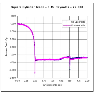
flow are presented in Fig. 3-5. Some local information for pressure distribution on the surface Fig. 6
Fig. 3 – Instantaneous Iso-Mach and streamlines
Table 1 - Cs influence
The influence of the Cs constant was investigated
using the reference solution and global parameters as indicators for the accuracy of the results, presented in
Table 1. The higher the values for the Cs constant, the
lower the St number is, with an constant increase in the drag coefficient, combined with lower oscillations in lift and drag. It is a logical trend that is based on the
constant increase in numerical viscosity through the Cs
coefficient. The value of Cs = 0.10 and Prt = 0.92 is a
confirmation for other similar numerical experiments.
Fig. 4 – Turbulent kinetic energy k
Fig. 5 – Instantaneous vorticity contours
A separate analysis was performed in order to investigate the influence of the definition of the filter length from (7). There was no significant changes in the global parameters considered, but one can identify some changes in other parameters. For instance, if one choose to plot the ratio of the turbulent viscosity/laminar viscosity, there is a difference in the field distribution of this parameter (mainly close to the solid walls) as well as in the rage of the values. However, it is not possible yet to decide what definition to use based on the current results. The first definition will be used in the next steps.
S qua re Cylinde r Ma c h = 0 . 15 Re ynolds = 2 2 . 0 0 0
-2.500 -2.000 -1.500 -1.000 -0.500 0.000 0.500 1.000 1.500
0.00 0.25 0.50 0.75 1.00 1.25 1.50 1.75 2.00 surf ace coordonat e
Cp-upper side Cp-lower side
Fig. 6 – Time averaged pressure distribution
The dynamic model was tested and compared with the standard one, using the same parameters as for the reference solution. The global values were close to the reference ones, but somehow worst if compared to the experimental values. The Strouhal number was
0.142, so 7.5% higher, and drag was Cd = 2.35,
dynamic model has to be triggered properly for every problem. It is also possible that more smoothing cycles and/or a different clipping procedure may give better results. All comments also have to be based on the imposed values for the beta-gamma scheme that may influence these findings.
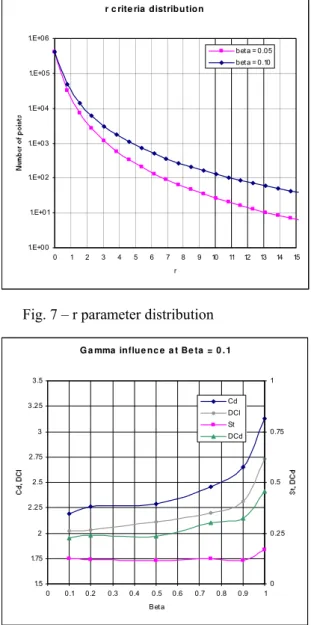
r c rite ria distribution
1.E+00 1.E+01 1.E+02 1.E+03 1.E+04 1.E+05 1.E+06
0 1 2 3 4 5 6 7 8 9 10 11 12 13 14 15 r
bet a = 0.05 bet a = 0.10
Fig. 7 – r parameter distribution
G a mma influe nc e a t Be ta = 0 . 1
1.5 1.75 2 2.25 2.5 2.75 3 3.25 3.5
0 0.1 0.2 0.3 0.4 0.5 0.6 0.7 0.8 0.9 1 Bet a
0 0.25 0.5 0.75 1
Cd DCl St DCd
Fig. 8 – Gamma influence at beta = 0.1
The numerical scheme was investigated using standard Smagorinsky model and the reference solution as
initial values. Then, both β and γ parameters were
changed and new solutions were computed. For a fixed
value of γ = 0.5, the upwind β parameter was modified
from 0.01 to 0.3. The values for the global parameters
are presented in Fig. 7. Also, for a fixed value of β
=0.1, the γ parameter was modified from 0.1 to 1.0 .
Results are presented in Fig. 8. From these results it is clear that the numerical scheme has a strong influence and the indicator introduced by (16) can be used to have more information on this effect.
If we compare the results with the incompressible case considered, one concludes that lower values for
both β and γ have to be used in order to match the
experimental data. However, one can see that several
combinations for β and γ may provide good results,
so further analysis may be considered in order to use
LES with upwind schemes. From the r indicator, one
can see that the distribution of the r in the field is
very interesting, with only 0.1% of the points with values above the average value of 0.118, as in Fig. 6. This indicator also requires further investigation in order to confirm these results.
Be ta influe nc e a t G a mma = 0 . 5
1.5 1.75 2 2.25 2.5 2.75 3 3.25 3.5
0 0.05 0.1 0.15 0.2 0.25 0.3 Bet a
0 0.05 0.1 0.15 0.2 0.25 0.3 0.35 0.4
Cd DCl St DCd
Fig. 9 – Beta influence at gamma = 0.5
The 3D aspects of the numerical discretization were investigated using 3 levels of spanwise distributions, from 10 to 30 planes in this direction. The results show that there are no significant changes with the increase in resolution in this direction, but this is because of the fact that the grid was still very coarse in this direction as compared to the main flow direction. The computational effort was however important, mainly for the 1.5 million point simulation.
8. Some conclusions
numerical results, some preliminary conclusions can be formulated, as follows:
• It is possible to use β-γ scheme for LES
compressible flows with the appropriate selection of their values. It is obvious that for very low
compressible flows, both β and γ has to be as low
as possible. On the other hand, for higher Mach numbers, one might expect to preserve the properties of the upwinding even for LES
modeling, with a selection around (β, γ ) = (0.1,
0.5). More numerical experiments and validations with experimental data have to be performed in order to validate this conclusion.
• Time step integration scheme has to be explicit,
because large CFL implicit numbers tend to act like filter in time on the solution. Also, since one is interested in LES for highly unsteady flows, non/reacting multifluid, etc., this seems the right choice. On the other hand, one has to remember that such simulations are very time consuming, not mainly because of the size of the domain, but because of the time development of the solution.
• There was no significant difference between the
standard and the dynamic LES model for the global parameters in the flow. If we consider that the dynamic model requires approx. 15% more time during the simulations, then we conclude that for rather simple flows, the standard model should be used. More investigations have to be performed in this direction either.
• Wall laws can be used in LES if there is no better
option. The implementations seams to comply with the experimental data and there are no problems concerning convergence. However, the fact that such laws are filtered in time and LES is using spatial filtering remains a problem.
• The global efficiency of the code using LES is as
good as for the k-ε, even better if we consider
memory allocation and I/O time. This conclusion is valid only for unsteady flows, where one has to compute long time cvasiperiodic solutions, so that time averaging is not an extra option. We believe that LES under presented form, for the test case, is
even more robust than standard k-ε model.
All the preliminary conclusions are coming from simulations on the test case. More investigations are required for other test configurations for complex geometries and for multifluid non/reacting flows.
REFERENCES
[1] W. RODI, J.H. FERZINGER, M. BREUER, M. POURQUIE, “Status of Large Eddy Simulation : Results of a
Workshop”, Transactions of ASME, 119, 248-262,
(1997)
[2] W. REHM, M.GERNDT, W. JAHN, R. VOGELSANG, B. BINNINGER, M. HERRMANN, H. OLIVIER, M. WEBER, “Reactive Föow Simulation in Complex Geometries
with High-Performance Supercomputing”, SNA
2000 Conference, Tokyo, Japan, 2000.
[3] O.V. VASILYEV, T.S. LUND, “A general theory of
discrete filtering for LES in complex geometry”,
Annual Research Briefs 1997, Center for Turbulence Research, NASA Ames/Standford Univ., 67-82, (1997)
[4] R. CARPENTIER, “Comparaison entre des schemas 2D de type Roe sur maillage regulier triangle ou quadrangle. II: calcul au sommet – Le β - γ schema”, INRIA N-3360, (1998)
[5] P.L. ROE, “Approximate Riemann Solvers, Parameters
Vectors and Difference Schemes”, J.C.P. Vol.43,
(1981)
[6] B. VAN LEER, “Flux Vector Splitting for the Euler equations”, Lecture notes in Physics, 170, (1982) [7] M. GERMANO, U. PIOMELLI, P. MOIN AND W. CABOt, “A
dynamic subgrid-scale eddy viscosity model”, Phys.
Fluids A3(7), (1991)
[8] D.A. LYN, S. EINAV, W. RODI, “A laser-Doppler velocimeter study of ensamble-averagd characteristics of the turbulent near wake of a square cylinder”, J. Fluid Mech., 304, (1995)
[9] C. NAE, “Flow Solver and Anisotropic Mesh Adaptation using a Change of Metric based on Flow
Variables”, AIAA Paper 2000-2250, (2000)
[10] K. SCHLOEGEL, G. KARYPIS AND V. KUMAR, “A Unfied Algorithm for Load-balancing Adaptive Scientific
Simulations“, Army HPC Research Center/ University