ISSN 1549-3636
© 2008 Science Publications
Calculate Sensitivity Function Using Parallel Algorithm
Hamed Al Rjoub
Irbid National University, Irbid, Jordan
Abstract:Problem statement: To calculate sensitivity functions for a large dimension control system using one processor, it takes huge time to find the unknowns vectors for a linear system, which represents the mathematical model of the physical control system. This study is an attempt to solve the same problem in parallel to reduce the time factor needed and increase the efficiency. Approach: Calculate in parallel sensitivity function using n-1 processors where n is a number of linear equations which can be represented as TX = W, where T is a matrix of size n1xn2, X = T
−1
W, is a vector of unknowns and X/ h = T−1 (( T/ h)-( W/ h)) is a sensitivity function with respect to variation of system components h. The parallel algorithm divided the mathematical input model into two partitions and uses only (n-1) processors to find the vector of unknowns for original system x = (x1,x2,…,xn)T and
in parallel using (n-1) processors to find the vector of unknowns for similar system (x')t = dtT−1 = (x1',x2',…xn')
T
by using Net-Processors, where d is a constant vector. Finally, sensitivity function (with respect to variation of component X/ hi = (xi×xi') can be calculated in parallel by
multiplication unknowns Xi×Xi', where i = 0,1,…n-1. Results: The running time t was reduced to
O(t/n-1) and, The Performance of parallel algorithm was increased by 40-55%. Conclusion: Used parallel algorithm reduced the time to calculate sensitivity function for a large dimension control system and the performance was increased.
Key words: Sensitivity Function, parallel, linear equations, variation, running time, mathematical model
INTRODUCTION
The ability to develop mathematical models in Biology, Physics, Geology and other applied areas has pull and has been pushed by, the advances in High Performance Computing. Moreover, the use of iterative methods has increased substantially in many application areas in the last years[9]. One reason for that is the advent of parallel Computing and its impact in the overall performance of various algorithms on numerical analysis[1].The use of clusters plays an important role in such scenario as one of the most effective manner to improve the computational power without increasing costs to prohibitive values. However, in some cases, the solution of numerical problems frequently presents accuracy issues increasing the need for computational power. Verified computing provides an interval result that surely contains the correct result. Numerical applications providing automatic result verification may be useful in many fields like simulation and modeling. Finding the verified result often increases dramatically the execution time[2]. However, in some numerical problems, the accuracy is mandatory. The requirements for achieving this goal are: interval arithmetic, high accuracy combined with well suitable algorithms. The
procedure is clearly an important consideration-so too is the accuracy of the method. Let us consider a system of linear algebraic equations:
AX = B (1)
Where:
A = {aij} ni ,j = 1 is a given matrix
B = (b1, ..., bn)t is a given vector
It is well known (for example[4,5]) that the solution, x, x Rn, when it exists, can be found using-direct methods, such as Gaussian elimination and LU and Cholesky decomposition, taking O(n3) time; -stationary iterative methods, such as the Jacobi, Gauss- Seidel and various relaxation techniques, which reduce the system to the form:
x Lx f= + (2)
and then apply iterations as follows: (0) (k ) (k 1)
x =f , x =Lx − +f , k 1, 2= (3)
until desired accuracy is achieved; this takes O(n2) time per iteration. -Monte Carlo methods (MC) use independent random walks to give an Approximation to the truncated sum (3):
1 (1) k
k 0
x L f
=
= (4)
Taking time O(n) (to find n components of the solution) per random step. Keeping in mind that the convergence rate of MC is 1/ 2
O(N− ), where N is the number of random walks, millions of random steps are typically needed to achieve acceptable accuracy. The description of the MC method used for linear systems can be found in[6-8]. Different improvements have been proposed, for example, including sequential MC techniques[5], resolve-based MC methods[1] and have been successfully implemented to reduce the number of random steps. In this study we study the Quasi-Monte Carlo (QMC) approach to solve linear systems with an emphasis on the parallel implementation of the corresponding algorithm. The use of quasirandom sequences improves the accuracy of the method and preserves its traditionally good parallel efficiency.
MATERIALS AND METHODS
Solution of large (dense or sparse) linear systems is considered an important Part of numerical analysis and
algorithms using this kind of routines is much larger than the execution time of the algorithms, which do not use it[11,10]. The C-XSC library was developed to provide functionality and portability, but early researches indicate that more optimizations may be done to provide more efficiency, due to additional computational cost in sequential and consequently for other environments as Itanium clusters. Some experiments were conducted over Intel clusters to parallelize self-verified numerical solvers that use Newton-based techniques but there are more tests that may be done.
Sensitivity analysis defines the relative sensitivity function for time independent parameters as:
i, j i i
S = ∂x / h∂ (5)
Where:
Xi = The i-th state variable
hj = The element of the parameter vector
Hence the sensitivity is given by the so-called sensitivity matrix S, containing the sensitivity coefficient Si,j, Eq. 5 The direct approach of
numerically differentiating by means of numerical field calculation software will lead to diverse difficulties[1,3]. Therefore, some ideas to overcome those problems aim at performing differentiations necessary for sensitivity analysis prior to any numerical treatment. Further calculations are then carried out with a commercially available field calculation program. Such approach has already been practical successfully[7].
We consider the linear system (1) where A is a tridiagonal matrix of order n of the form shown in (6),
T 0 1 n 1
x=(x , x ,..., x −) is the vector of unknowns and
T 0 1 n 1
d=(d , d ,...,d −) is a vector of dimension n:
o o
1 1 1
2 2 2
n 1 n 1 n 1
n 1 n 1
b c
a b c
a b c A
.. ..
a b c
a b
− − −
− −
= (6)
In the LU factorization A , is decomposed into a product of two bidiagonal matrices L and U as A = LU, where:
1
n
2
n 1
1
h 1
.. 1
L .. ..
h 1
h 1
−
−
=
0 0
1 1
n 2 n 2
n 1
U C
U C
U
U C
U
− − −
− −
=
− −
The LU algorithm to solve the linear system (1) then proceeds to solve for y from Ly=d and then finds vector X in parallel:
Step 1: Compute the decomposition of A given by:
0 0
i i i
i i i i 1
u b
h a / u 1,1 i n 1,
u b h *c−1 i n 1
=
= − <= <= −
= − < = < = −
Step 2: Solve for y from Ly = d using:
0 0
i i i i 1
y d
y d h *y ,1− i n 1
=
= − <= <= −
Step 3: Compute X by solving ux = y using:
n 1 n 1 n 1
i i i i 1 i
X Y / U ,
X (Y C *X ) / U ,0 i n 2
− − −
+
=
= − <= <= −
First we consider the parallelization of the LU decomposition part of the LU algorithm to solve (1), i.e., Step 1 above. Once the diagonal entries u0,u1,…,un
of U have been calculated, h1,h2,…,hn-1can
subsequently be computed in a single parallel step with n-1 processors. Thus we concentrate on the computation of the ui's.
RESULTS
time on m for both single and multi thread versions, for single thread we start basic multiplication division and subtraction inside the Matrix until we get the upper of that matrix, for multi threading we use R-1 threads where R is the count of desired Matrix rows, we measured the longest thread which is the last one in our case, then every thread takes a part of the Matrix basic operations and we do that in parallel for origin and similar systems.
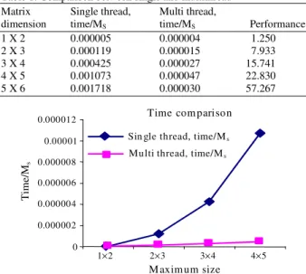
Table 1 shows the time results done on Pentium Due 1.8 GHZ processor with 1 GB Ram and shows the time when we use one processor (single thread) and the time when we use a multi processors in parallel (multi thread) to calculate the unknowns vector. From the Table 1, Fig. 1 and 2, we can see that performance increase with respect to the size of matrix, which represents the linear system.
Table 1: Comparison between single and multithread
Matrix Single thread, Multi thread,
dimension time/MS time/MS Performance
1 X 2 0.000005 0.000004 1.250
2 X 3 0.000119 0.000015 7.933
3 X 4 0.000425 0.000027 15.741
4 X 5 0.001073 0.000047 22.830
5 X 6 0.001718 0.000030 57.267
0 0.000002 0.000004 0.000006 0.000008 0.00001 0.000012
1×2 2×3 3×4 4×5
T
im
e/
Ms
M axim um size Time com parison
Sin gle thread, time/Ms Multi thread, time/Ms
Fig. 1: Time comparison between single and parallel to calculate unknowns vector
Performance doubling
0.000 0.050 0.100 0.150 0.200 0.250
1×2 2×3 3×4 4×5
S
p
ee
d
d
o
u
b
li
n
g
Maximum size Performance
Fig. 2: System performance chart
DISCUSSION
The time to find in parallel unknown vector was decreased with respect to the increased size of the matrix, which represent the mathematical model of physical system (Table 1),and with respect to the single thread , the performance was increased (Fig. 1 and 2). The main goal of Parallel algorithm is resolving in parallel linear equations which represents as AX = W and calculate sensitivity function of electric power systems to obtain the result with respect to variation any component of output function F with respect to any component of electric power systems h( f / h)∂ ∂ .
Parallel algorithm contains the next stages: distribution data (rows matrix T and components vector W) to the p processors where p= n-1 (n is the number of equations) which represents the mathematical model of electric system and calculate in parallel unknown vector for
origin system T
1 2 n
X (x , x ,..., x )= . Distribution data (at
the same time) to p processors and calculate unknown vector for similar system I t t 1 I I T
1 2 n
(x ) = −d T− =(x , x ,..., x )Ι .
Multiplication operation for unknown's xi × x|i
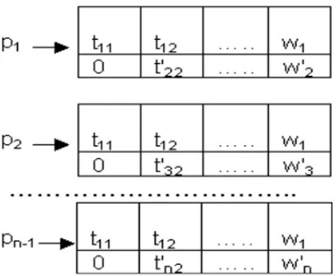
respectively using p processors to find in parallel sensitivity function for a large dimension system. Distribution data stage: In this stage, given first row matrix T and the first component of right side linear equation TX = W (w1)to the first processor p1 ,and first
row with component w1 to second processor p2 and first
row with component w1 to third processor ,and first row
with component w1 to the pn-1 processor. Figure 3
shows this stage.
Given p1 second row matrix T with component w2,
p2 third row matrix T with component w3 and pn-1 last
row matrix T with component wn (Fig. 4).
Fig. 3: Distribution first row matrix T and w1
Fig. 5: Multiply first rows (p1, p2, pn-1) by Constants
c1,c2,cn-1 respectively
Fig. 6: Distribution rows between processors, where p = n-2 (working in parallel)
Fig. 7: Representation of the final step on processor p1
Multiplication Stage: Multiply the first row processors p1, p2, pn-1 by constants c1,c2,cn-1 respectively and
subtract second row components from the result to obtain zero in the first component of the second rows Fig. 5.
The second row processor p1 become the first row
for all processors, where the number of processors is equal n-2 (Fig. 6).
After n-1 cycles of multiplication operation and distribution rows between processors, just on p1 we
obtained a system, which contains tow rows. Figure 7 shows the final step.
Finally we get the mathematical model for original system as triangular equations:
11 12 1n 1 1
22 2n 2 2
3n 3
(n 1)n n n
t t ... t X W
0 t ... t X W
0 0 ... t ... W
0 0 0 tt − X W
′ ′ × = ′
′ ′′
′′′
The above triangular equations are solved by back substitution. From the last equation, we immediately have xn=W′′′n/ tt(n 1)n− . By substituting this value in the
n-1 equation, we find xn-1 and so onwe find unknown
vector for original system T
1 2 n
X (x , x ,..., x )= .
Distribution data for similar system: Distribute data to p = n-1 processors and calculate unknown vector for similar system I t t I I I I
1 2 n
(x ) =d T =(x , x ,...,x ), (we do that at
the same time when we calculated unknown vector for
original system T
1 2 n
X (x , x ,..., x )= as mentioned above ).
Calculate in parallel sensitivity function algorithm: Step 1: Compute unknown vector for similar system
| | | |
1 2
X (x ,x ,...,x )
=
using next equation:| 1
(x )t= −dT−
(7)
Step 2: Multiplicate Eq. (7) from the right side by matrix T and transpose left and right side to obtain a system with respect to |
x:
t |
T X= −d (8)
Step 3: Calculate:
X / h T 1( T / h)X ( W / h)
∂ ∂ = − − ∂ ∂ − ∂ ∂ (9)
Step 4: Find sensitivity Function f with respect to h:
t 1
j / h d T ( T / W / h)−
∂ ∂ = − ∂ ∂ ∂ (10)
Step 5: Put the expression (6) in (9) then:
| t | t
j / h (x ) T / hX (x ) W / h
∂ ∂ = ∂ ∂ − ∂ ∂ (11)
To use the expression (11) we just need to resolve in parallel the tow linear systems (1) and (8) by using parallel algorithm.
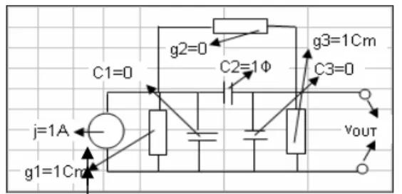
A numerical example: Figure 8 shows the electric circuit, in which we wont to calculate in parallel the sensitivity function of the output potential vout with
respect to resistance g2, condensers c1 and c3,
respectively, the mathematical model for this circuit is:
1 2 S 1 S 2 2 S 2 1
2 S 2 2 3 S 2 S 3 2
1
G G C C G C V
0
G C G G C C V
+ + + −
× =
Fig. 8: Electric circuit to calculate sensitivity function for vout with respect to variation parameters (C1,
G2, C3)
Using PNPA algorithm in parallel, we find unknowns vector X for original system:
1 2
(3 j) / 5 v
x
(2 j) / 5 v
−
= =
+
At the same time we find unknowns vector X| for similar system:
| | 1
| 2
(2 j) / 5 v
x
( 3 j) / 5 v
− +
= =
− +
Finally we just do the multiplication operation to find the sensitivity function as follows:
| out 1 1 1
| |
out 2 1 2 1 2
| out 3 2 2
V / C s V v 1 j7 / 25
V / G (V v )(V v ) 3 j4 / 25
V / C sV v 1 j7 / 25
∂ ∂ = = −
∂ ∂ = − − = − −
∂ ∂ = = −
CONCLUSION
The parallel algorithm to find the vector of unknowns for calculated in parallel sensitivity function and one thread was simulated and proved that parallel algorithm is more efficient. The running time was reduced to O(t/n-1) and the efficiency was increased by 40-55%.
ACKNOWLEDGMENT
The researcher acknowledge the financial support (Fundamental Research Scheme) received from Irbid National University, Irbid, Jordan.
REFERENCES
1. Duff, I.S. and H.A. van de Vorst, 1999. Developments and trends in parallel solution of linear systems. Paral. Comput., 25: 1931-1970. DOI: 10.1016/S0167-8191(99)00077-0
2. Ogita, T., S. M. Rump and S. Oishi, 2005. Accurate sum and dot product. SIAM. J. Sci. Comput., 26: 1955-1988. http://www.ti3.tu-harburg.de/paper/rump/OgRuOi05.pdf
3. Li, G. and T.F. Coleman, 1989. A new method for solving triangular system on distributed memory message-passing multiprocessors. SIAM J. Sci. Stat. Comput., 10: 382-396. DOI: 10.1137/0910025
4. Duff, I.S., 2000. The Impact of High Performance Computing in the solution of linear systems: Trend and proplems. J. Comput. Applied Math., 123: 515-530.
DOI: 10.1016/S0377-0427(00)00401-5
5. Liu, Z. and D.W. Cheung, 1997. Efficient parallel algorithm for dense matrix LU decomposition with pivoting on hypercubes. J. Comput. Math. Appl., 33: 39-50. DOI: 10.1016/S0898-1221(97)00052-7 6. Pan, V. and J.Reif, 1989. Fast and efficient parallel
solution of dense linear system. Comput. Math.
Appl., 17: 1481-1491.
http://cat.inist.fr/?aModele=afficheN&cpsidt=7227240
7. Eisentat, S.C. and M.T. Heath, 1988. Modified cyclic algorithm for solving triangular system on distributed-memory multiprocessor. SIAM J. Sci. Stat. Comput., 9: 589-600. DOI:10.1137/0909038 8. Holbig, C.A. and P.S. Morandi, 2004. Selfverifying
solvers for linear systems of equations in C-XSC. Lecture Notes Comput. Sci., 3019: 292-297.
http://cat.inist.fr/?aModele=afficheN&cpsidt=15811200
9. Singer, M.F., 1988. Algebraic relations among solutions of linear di-erential equations: Fano's theorem. Am. J. Math., 110: 115-143. http://www.jstor.org/pss/2374541
10. Saad, Y., 1996. Iterative methods for sparse linear systems. Proceeding of the Symposium on FPGAs, (FPGAs’96), ACM Press, New York, USA., pp: 157-166.