Estados Exóticos do Charmonium

(1)

!

! ! !

UNIVERSITÉ!MONTPELLIER!2!!!!!!!!!!!!!!!!!!!!!!!!!!!!!!!!!!!!!!!!!!!!!!!!!!!!!!!!!!!!!!!!!!!!!!!!!!!!!!!!!UNIVERSITÉ!SÃO!PAULO! Sciences!et!Techniques!du!Languedoc!!!!!!!!!!!!!!!!!!!!!!!!!!!!!!!!!!!!!!!!!!!!!!!!!!!!!!!!!!!!!!!!!!!!!!!!!!!!Institut!de!Physique! France!!!!!!!!!!!!!!!!!!!!!!!!!!!!!!!!!!!!!!!!!!!!!!!!!!!!!!!!!!!!!!!!!!!!!!!!!!!!!!!!!!!!!!!!!!!!!!!!!!!!!!!!!!!!!!!!!!!!!!!!!!!!!!!!!!!!!!!!!!!!!!!!!!!!!!!!!!!!!!!!!!!Brésil!

!

THESE!de!DOCTORAT!!

(en$COTUTELLE)$

pour!obtenir!le!grade!de!

DOCTEUR!DE!L'UNIVERSITE!MONTPELLIER!2!6!FRANCE!

Spécialité:* Physique!

Ecole*Doctorale:* I2S!G!Information,!Structures!and!Systèmes! Laboratoire*d'accueil:* LUPMGUM2!

!

DOCTEUR!DE!L'UNIVERSITE!SAO!PAULO!6!BRESIL!

Spécialité:* Physique!

Ecole*Doctorale:* Sciences!Exactes!et!Naturelles! Laboratoire*d'accueil:* IFGUSP!

!

présentée!et!soutenue!publiquement!par:!

Raphael!Moreira!de!ALBUQUERQUE!

le!18!Février!2013!

_____________________________________________________________________________________________!

ETATS!EXOTIQUES!DU!CHARMONIUM!

_____________________________________________________________________________________________! !

Devant!le!JURY!composé!de:!

(2)

(3)

!

! ! !

UNIVERSITÉ!MONTPELLIER!2!!!!!!!!!!!!!!!!!!!!!!!!!!!!!!!!!!!!!!!!!!!!!!!!!!!!!!!!!!!!!!!!!!!!!!!!!!!!!!!!!UNIVERSITÉ!SÃO!PAULO! Sciences!et!Techniques!du!Languedoc!!!!!!!!!!!!!!!!!!!!!!!!!!!!!!!!!!!!!!!!!!!!!!!!!!!!!!!!!!!!!!!!!!!!!!!!!!!!Institut!de!Physique! France!!!!!!!!!!!!!!!!!!!!!!!!!!!!!!!!!!!!!!!!!!!!!!!!!!!!!!!!!!!!!!!!!!!!!!!!!!!!!!!!!!!!!!!!!!!!!!!!!!!!!!!!!!!!!!!!!!!!!!!!!!!!!!!!!!!!!!!!!!!!!!!!!!!!!!!!!!!!!!!!!!!Brésil!

! ! !

!

! ! !

Universidade de S˜

ao Paulo

Instituto de F´ısica

Estados Ex´

oticos do Charmonium

Raphael Moreira de Albuquerque

Tese de doutorado apresentada ao Instituto

de F´ısica da Universidade de S˜ao Paulo para

a obten¸c˜ao do t´ıtulo de Doutor em Ciˆencias.

Orientadores :_Profa

. Dra

. Marina Nielsen (Univ. S˜ao Paulo, Brasil)

Prof. Dr. Stephan Narison (Univ. Montpellier 2, Fran¸ca)

Banca Examinadora :

Profa

. Dra

. Marina Nielsen (Univ. S˜ao Paulo, IFUSP - Brasil)

Prof. Dr. Stephan Narison (Univ. Montpellier 2, LUPM - Fran¸ca)

Prof. Dr. Fernando Silveira Navarra (Univ. S˜ao Paulo, IFUSP - Brasil)

Prof. Dr. Jean-Marc Rene Richard (Univ. de Lyon, IPNL - Fran¸ca)

Prof. Dr. Ricardo D’Elia Matheus (Univ. Estadual Paulista, IFT - Brasil)

S˜

ao Paulo, 2012

!

(4)

FICHA CATALOGRÁFICA

Preparada pelo Serviço de Biblioteca e

Informação

do Instituto de Física da Universidade de São

Paulo

Albuquerque, Raphael Moreira de

Estados Exóticos do Charmonium. – São Paulo, 2013.

Tese (Doutorado) – Universidade de São Paulo. Instituto de Física – Depto. de Física Experimental

Orientador: Profa. Dra. Marina Nielsen Co-Orientador: Prof. Dr. Stephan Narison

Área de Concentração: Física

Unitermos: 1.Física; 2. Física de partículas;

3.Interações fundamentais; 4. Cromodinâmica quântica; 5. Teoria quântica de campos.

(5)

(6)

(7)

Laboratoires d’accueil :







Le projet de recherche de cette thèse a été soutenu par :

(8)

(9)

Langue de R´edaction du Manuscrit

Cette thèse a été réalisée sous la “Convention de Cotutelle de Thèse” approuvée par

le Conseil Scientifique pl´enier du 7 juillet 2011. Cette Convention r´eglemente les

rela-tions entre l’Universit´e de Montpellier 2 Sciences et Techniques (Montpellier, France)

représentée par son Président Madame le Professeur Danièle HERIN, conformément à

l’arrêté du 6 janvier 2005, régissant les cotutelles internationales de thèses, et l’Université

de São Paulo (São Paulo, Brésil) représentée par son Président Monsieur le Professeur

João Grandino Rodas, conformément à législation du pays concerné.

L’Article 2 du Titre II - Modalités Pédagogiques de cette Convention prévoit que :

“... La thèse sera rédigée et soutenue en langue Anglais_{. Lorsque les langues nationales}

des deux pays concernés sont différentes, le doctorant est tenu de compléter la thèse par

un résumé écrit et oral dans l’autre langue. Le doctorant établira le résumé en langue :

(10)

(11)

To my beloved family,

Ademir, Hilda, F´abio and Dany,

and to my dearest love and best friend,

(12)

(13)

R´esum´e

Cette thèse a utilisé la méthode des règles de somme de QCD pour étudier la nature

des r´esonances du charmonium suivantes : Y(3930),Y(4140),X(4350),Y(4260),Y(4360)

et Y(4660). Il y a des fortes indications que ces ´etats ont des structures hadroniques

non conventionnelles (ou exotiques) lorsque leurs masses respectives et les modes de

désintégration observés expérimentalement sont incompatibles avec ce qui est attendu

pour l’état conventionnel du charmonium (c¯c). Le même phénomène se produit dans le

secteur du bottomonium (b¯b), où les nouveaux états Yb(10890) et Yb(11020) observées

r´ecemment pourraient indiquer l’existence de nouveaux ´etats exotiques du bottomonium.

De cette fa¸con, on vérifie que l’état Y(4140) peut être décrit soit par une structure

mol´eculaire D∗

sD¯∗s (0++) ou par une mélange entre les états moléculaires D∗sD¯∗s (0++)

et D∗_D¯∗ ₍₀++_{). Les états} _Y_{(3930) et} _X_{(4350) ne peuvent pas être décrites par les}

cou-rants mol´eculaires D∗_D¯∗ ₍₀++_{) et} _D∗

sD¯∗s0 (1−+), respectivement. On v´erifie ´egalement que

la structure mol´eculaire ψ′ _f

0(980) (1−−) réproduit très bien la masse de l’état Y(4660).

Une extension naturelle au secteur du bottomonium indique que l’´etat mol´eculaire

Υ′f0(980) est un bon candidat pour l’´etatYb(10890). On a ´egalement fait une estimation

pour les états moléculaires possibles formées par des mésons D et B, ce qui pourra être

observ´e dans des exp´eriences futures au LHC.

Une vaste ´etude, en utilisant le formalisme habituel des r`egles de somme et aussi le

Double Rapport des R`egles de Somme, est fait pour calculer les masses des baryons lourds

en QCD. Les estimations pour les masses des baryons avec un (Qqq) et deux (QQq) quarks

lourds sont un excellent test pour la capacité de la méthode de règles de somme à prédire

les masses des baryons qui n’ont pas encore été observés.

Mots-clés :QCD, Physique des Particules, Physique Hadronique, Phénoménologie, Baryons et

(14)

(15)

Abstract

In this thesis, the QCD sum rules approach was used to study the nature of the following

charmonium resonances: Y(3930), Y(4140), X(4350), Y(4260), Y(4360) and Y(4660).

There is strong evidence that these states have non-conventional (or exotic) hadronic

structures since their respective masses and decay channels observed experimentally are

inconsistent with what expected for a conventional charmonium state (c¯c).

The same phenomenon occurs on the bottomonium sector (b¯b), where new states like

Yb(10890) and Yb(11020) observed recently could indicate the existence of new

bottomo-nium exotic states. In this way, one verifies that the stateY(4140) could be described as a

D∗

sD¯∗s (0++) molecular state or even as a mixture ofDs∗D¯∗s (0++) andD∗D¯∗ (0++)

molec-ular states. For the Y(3930) and X(4350) states, both cannot be described as a D∗_D_¯∗

(0++_{) and} _D∗

sD¯s∗0 (1−+), respectively. From the sum rule point of view, theY(4660) state

could be described as aψ′f0(980) (1−−) molecular state. The extension to the

bottomo-nium sector is done in a straightforward way to demonstrate that theΥ′_f

0(980) molecular

state is a good candidate for describing the structure of theYb(10890) state. In the

follow-ing, one estimates the mass of the exotic Bc-like molecular states using QCD Sum Rules

- these exotic states would correspond to bound states of D(∗) _and _B(∗) _{mesons. All of}

these mass predictions could (or not) be checked in a near future experiments at LHC.

A large study using the Double Ratio of Sum Rules approach has been evaluated for

the study of the heavy baryon masses in QCD. The obtained results for the unobserved

heavy baryons, with one (Qqq) and two (QQq) heavy quarks will be an excellent test for

the capability of the sum rule approach in predicting their masses.

Keywords: QCD, Particle Physics, Hadronic Physics, Phenomenology, Baryons and Mesons, QCD

(16)

(17)

Resumo

Nesta tese ´e utilizado o m´etodo das Regras de Soma da QCD para estudar a

natu-reza dos seguintes estados ressonantes do charmonium: Y(3930), Y(4140), X(4350),

Y(4260),Y(4360) eY(4660). H´a fortes evidˆencias de que estes estados possuam estruturas

hadrônicas não convencionais (ou exóticas) uma vez que as suas respectivas massas e

ca-nais de decaimento observados experimentalmente s˜ao inconsistentes com o que ´e esperado

para o estado ressonante convencional do charmonium (c¯c). O mesmo fenˆomeno ocorre

no setor do bottomonium (b¯b), onde os novos estados Yb(10890) e Yb(11020) observados

recentemente poderiam indicar a existˆencia de novos estados ex´oticos do bottomonium.

Neste sentido, verifica-se que o estado Y(4140) pode ser descrito ou por uma estrutura

molecular D∗

sD¯∗s (0++) ou mesmo uma mistura entre os estados moleculares D∗sD¯s∗ (0++)

eD∗_D¯∗ ₍₀++_{). J´a os estados} _Y_{(3930) e o} _X_{(4350) n˜ao podem ser descritos por correntes}

moleculares D∗_D¯∗ ₍₀++_{) e} _D∗

sD¯∗s0 (1−+), respectivamente. Verifica-se tamb´em que a

es-trutura molecularψ′_f

0(980) (1−−) descreve muito bem a massa do estadoY(4660). Uma

extens˜ao ao setor do bottomonium indica que o estado molecular Υ′ _f

0(980) ´e um bom

candidato para descrever a estrutura do estado Yb(10890). ´E feita tamb´em uma

estima-tiva para os poss´ıveis estados moleculares formados por m´esons D e B, que poder˜ao ser

observados em futuros experimentos realizados pelo LHC.

Um amplo estudo, utilizando o formalismo das Regras de Soma e tamb´em da Dupla

Razão das Regras de Soma, é feito para calcular as massas dos bárions pesados na QCD.

As estimativas para as massas dos b´arions com um (Qqq) e com dois (QQq) quarks pesados

s˜ao um excelente teste para a capacidade do m´etodo das regras de soma em prever a massa

dos b´arions que ainda n˜ao foram observados.

Palavras-chave: QCD, F´ısica de Part´ıculas, F´ısica Hadrônica, Fenomenologia, Bárions e Mésons,

(18)

(19)

Chapter 1 Introduction

In particle physics, a hadron is a composite particle made up of quarks and gluons

interacting via strong interactions. The hadrons are divided into two groups: mesons

(made of a quark-antiquark pair, or qq¯) and baryons (made of three quarks, or qqq).

The strong interactions, responsible for keeping quarks together inside the hadrons, are

described by a non-Abelian gauge theory called Quantum Chromodynamics (QCD) [1].

In QCD, the quarks and gluons are the fundamental particles which carry a

non-vanishing color charge. These particles interact with each other through the strong

interactions that are mediated by gluons. Note the analogy with Quantum

Electrody-namics (QED), where the particles with electromagnetic charge interact through photon

exchange [1]. However, QCD has some fundamental properties, such as asymptotic

free-dom and confinement, that make it a theory much more complex than QED.

In the early seventies, the physicists David Politzer, David J. Gross and Frank Wilczek

[2] proved that in QCD, the effective strong coupling constant vanishes at short distances

(high-energy regime) and increases at long distances (low-energy regime). The former

case implies that QCD becomes a weakly coupled theory (gs →0) and, in principle, can

be evaluated using perturbative methods. For the latter case, however, QCD becomes

a strongly coupled theory (gs $ 1) and the non-perturbative effects are expected to be

(24)

the most valuable contribution to the formation of the physical observables. This running

behavior of the strong coupling ”constant” is associated to an important property in QCD

known as asymptotic freedom.

Further analysis in QCD guarantees that the physical bound states must hold a color

singlet combination in order to satisfy the Pauli exclusion principle [1]. Since quark and

gluons carry the color charge and rather cannot be described by color singlet states, then

this could be an explanation for one has never seen them as free particles in the nature.

This feature is commonly associated with the confinement mechanism, which ensures that

quarks and gluons remain confined inside hadrons.

It is known that hadrons are color singlet states formed in the low-energy regime, and

the strong interactions between them are due to the meson exchange (e.g. pions, kaons),

instead of the gluon exchange. In this scenario, QCD is no longer able to adequately

describe hadrons and their interactions in terms of degrees of freedom of quarks and

gluons. Consequently, it is mandatory to construct physical models, which incorporate

these fundamental properties of QCD and describe the hadrons in a consistent way with

the experimental data.

One of these models, the so-called Constituent Quark Model (CQM), was proposed

by the physicists Murray Gell-Mann [3] and George Zweig [4]. The CQM is a successful

model which is widely used to classify hadrons and calculate their masses and decay

widths [5]. According to CQM, the mesons are particles composed of a quark-antiquark

pair (qiq¯i), whereas the baryons are particles composed of three quarks ($ijkqiqjqk). The

latin indices represent the colors of the quark fields. In nature, mesons and baryons must

be represented by color singlet states with a neutral color charge.

It is worth mentioning that, in addition to these conventional structures, QCD would

accept the existence of many other kinds of internal structures for hadrons, such as

glue-balls (gg, ggg, . . .) [6], hybrid states (qqg, qqqg, . . .¯ ) [7], hadronic molecules (DD, D¯ ∗_{D, . . .}_¯ ₎

(25)

1.1. CHARMONIUM EXOTIC STATES 3

usually related to the exotic states. Indeed, although the current studies on particle

physics reveal that the vast majority of observed hadrons are remarkably well described

by CQM, recent researches on charmonium (c¯c) spectroscopy, carried out by BaBar [13]

and Belle [14] collaborations, have indicated the possible existence of new mesons with a

structure much more complex than the conventional qq¯system.

1.1 Charmonium Exotic States

At the beginning of the XXI century, two main research centers began performing

experiments in order to test the CP symmetry violation in the Standard Model:

– BaBar collaboration at Stanford Linear Accelerator Collider, United States (SLAC),

– Belle collaboration at High Energy Accelerator Research Organization, Japan (KEK).

Both collaborations analyzed e+_e− _{collisions operating at a centre-of-mass energy (}_E

CM)

close to 10.6 GeV. In thisECM, there is a large production of BB¯ pairs, hence the name

B₋factories. The B mesons which are produced decay predominantly into channels

con-tainingcquarks and ¯cantiquarks, thus often exhibiting a significant presence of charmed

hadrons and charmonium (c¯c) in the final states.

The charmonium production at the B₋factories can also occur through a process

called Initial State Radiation (ISR). By using ISR process, an energetic photon is emitted

by either the initial electron or positron, it is possible to study not only the produced

events at the collider nominal ECM, but also at lower energies. When the energy of

irradiated photons (γISR) is in the range between 4.0 to 5.0 GeV, the e+e− annihilation

occurs in an ECM which corresponds to the mass region allowed for the excited states of

the charmonium c¯c.

According to CQM, widely used in the study of hadron spectroscopy, it was expected

that ISR processes could produce a large amount of phenomenological data on the 1−−

(26)

ψ(4415). However, the first 1−− _{resonant states produced experimentally by} _B₋_factories

were: Y(4260),Y(4360) andY(4660). In addition to having a mass incompatible with the

spectrum predicted by CQM, these states also present a decay pattern totally unexpected

for a conventional charmonium state.

Although in Ref. [15], the authors argue that the Y(4360) and Y(4660) are

conven-tional cc¯states, the 33_D

1 and 53S1 states respectively, their masses are inconsistent with

predicted by CQM in [5]. Besides, the absence of open charm production would be also

inconsistent with a conventional cc¯structure. A good review of these new states could

be found in Refs. [16, 17]. Facing this impasse between CQM theoretical predictions and

experimental data, it becomes necessary to build models where the structure for these

new charmonium states goes beyond the conventional c¯c structure. Clearly, one needs

further experimental data and theoretical development for a better understanding of the

properties of these new states.

In the present work, one uses the QCD Sum Rules approach (QCDSR), proposed in

1979 by M. Shifman, A.I. Vainshtein and V.I. Zakharov [18–20], to study whether these

new charmonium states have an exotic structure, like molecular states.

1.1.1 Y(4260), Y(4360) and Y(4660)

In 2005, the experiments based on ISR processes, carried out by BaBar collaboration,

indicated a resonant peak around 4300 MeV produced in the decay channel [21]:

e+e− _−→γISRY(4260)−→γISR J/ψ π

+_π− _.

The full width measured for the intermediateY(4260) state was approximately of 90 MeV.

The CLEO collaboration has also confirmed the observation of this state [22]. The

prox-imity between the Y(4260) mass and that obtained for ψ(4153) state led some authors

(27)

1.1. CHARMONIUM EXOTIC STATES 5 ) 2 ) (GeV/c ψ J/ -π + π m(

3.8 4 4.2 4.4 4.6 4.8 5

2

Events / 20 MeV/c

0 10 20 30 40 ) 2 ) (GeV/c ψ J/ -π + π m(

3.8 4 4.2 4.4 4.6 4.8 5

2

Events / 20 MeV/c

0 10 20 30 40 ) 2 ) (GeV/c ψ J/ -π + π m(

3.8 4 4.2 4.4 4.6 4.8 5

2

Events / 20 MeV/c

0 10 20 30 40 ) 2 ) (GeV/c ψ J/ -π + π m(

3.8 4 4.2 4.4 4.6 4.8 5

2

Events / 20 MeV/c

0 10 20 30 40

3.6 3.8 4 4.2 4.4 4.6 4.8 5 1 10 2 10 3 10 4 10 (a) 0 5 10 15

4 4.5 5 5.5

M(π+π-ψ(2S)) (GeV/c2)

Entries/25 MeV/c

2

(b)

Figure 1.1: The invariant-mass distribution of [13, 14]: a)J/ψ π+_π− _and_b)_ψ₍₂_S₎_π+_π−_.

the total width observed for the Y(4260) are not in agreement with expected by CQM

predictions for the charmonium resonances, which should decay into channels containing

predominantly D mesons and would have a width larger than 90 MeV. Thus, Maiani et

al. [23] have proposed that theY(4260) could be described as a tetraquark [cs][¯cs¯] state.

Recently, Belle collaboration not only confirmed the existence of the Y(4260) state

[25], but also announced the discovery of two other vector mesons [14], the Y(4360) and

Y(4660), whose resonant peaks are around 4360 MeV and 4660 MeV, respectively. Both

states are produced through the following process:

e+e− _−→γ_ISRψ′ π+π−.

with the same JP C _{= 1}−− _{quantum numbers. The measurements of the total widths}

for the Y(4360) and Y(4660) states are 74±18 MeV and 48±15 MeV, respectively [14].

With these values, either Y(4360) or Y(4660) states are consistent with conventional

charmonium states in this mass region. The invariant mass distributions obtained by

Belle and BaBar collaborations are shown in Fig.(1.1).

Important information for understanding the structure of these states is which resonant

intermediate state is responsible for producing the pair of pions in their respective decay

(28)

Figure 1.2: Dipion invariant mass spectrum of the decay channels [24]: Y(4260)→J/ψ π+_π− _(left),

Y(4360)→ψ(2S)π+π− _{(middle) and}_Y₍₄₆₆₀₎_→_ψ₍₂_S₎_π+_π− _(right).

the Y(4660) state presents a well defined intermediate state consistent with f0(980) [24].

Due to this fact and the proximity of the mass of the system ψ(2S)₋f0(980) with the

Y(4660) mass, in Ref. [26], the authors suggested that theY(4660) could be described by

the ψ(2S)f0(980) molecular state. There are also other interpretations for the Y(4660)

state like baryonium state [27] or a conventional charmonium state 53_S

1 c¯c [15]. For the

other two mesons, Y(4260) and Y(4360), Fig.(1.2) indicates that the ππ pairs in their

respective decay channel are more consistent with the σ(600) scalar meson [24, 28] than

the f0(980) meson.

In the present work [29], one uses the QCDSR approach to investigate if a correlation

function based on J/ψf0(980) or J/ψ σ(600) molecular currents, with JP C = 1−−, could

describe the structure of at least one of these new charmonium states.

1.1.2 Y

(4140)

The CDF collaboration found evidence for a new particle calledY(4140) [30] produced

by the particle accelerator Tevatron at FERMILAB. The signal of this particle, with

significance of 3.8σ, was seen in the decay ofB mesons with a mass M_Y₍₄₁₄₀₎ = (4143.0±

(29)

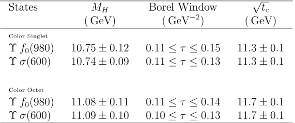
Figure 1.3: Evidence for observation of Y(4140) state by Belle collaboration [30]. One of the lines

(blue) represents the expected background composed of mesonsK (MKK ≃1.0 GeV), while the other

line with a peak (red) is the fit to events observed.

muons and kaons pairs:

B+ _→ Y(4140)K+

Y(4140) _→ J/ψ φ _→ µ+µ−K+K−. (1.1)

Since the Y(4140) state decays into two IG!

JP C"

= 0−(1−−) vector mesons, it has

positive C and G parities. There are already some theoretical interpretations for this

structure. Its interpretation as a conventional cc¯state is complicated because, as pointed

out by the CDF [30] and Belle [42] collaborations, it lies well above the threshold for open

charm decays and, therefore, a c¯c state with this mass would decay predominantly into

an open charm pair with a large total width. Then, they concluded that the Y(4140)

is probably a D∗

sD¯s∗ molecular state with JP C = 0++ or 2++. In Ref. [31], the authors

interpreted the Y(4140) as the molecular partner of the charmonium-like state Y(3930),

which was observed by Belle and BaBar collaborations near theJ/ψ ωthreshold [32, 33].

In Ref. [34], the authors have interpreted the Y(4140) as an exotic hybrid charmonium

(30)

There are many other works about the possible theoretical interpretations for the

Y(4140) state and more discussions can be found in Refs. [35–40].

In the present work [35], one uses the QCDSR approach to study if a two-point

cor-relation function based on a D∗

sD¯∗s molecular current, with JP C = 0++, can describe the

new observed resonant structure Y(4140).

1.1.3 Y(3930)

Another intriguing state is the so-called Y(3930). The Belle collaboration [32] has

announced the observation of this state in the decay channel B _→ Y(3930)K, with

significance of 8.1σ. This signal has also been confirmed by BaBar collaboration [33].

The experimental mass and total width are given by [41]: M_Y₍₃₉₃₀₎ = (3917.5±2.7) MeV

and Γ= (27±10) MeV.

If it were a conventional charmonium state, the Y(3930) state would decay

predom-inantly into D mesons since its mass is above the DD threshold. However, this state

decays dominantly through the following channel:

Y(3930)_→J/ψ ω . (1.2)

The Y(3930) state has a mass of approximately 200 MeV below the Y(4140) mass.

This difference could be related to the quarks constituting both particles. Note that the

difference between the quark masses is in order of: ms−mq ≃ 100 MeV. In this way,

the D∗_D¯∗ _{molecular state, with} _JP C _{= 0}++_{, is a good candidate to describe the}_Y₍₃₉₃₀₎

state.

cor-relation function based on a D∗_D_¯∗ _{molecular current, with} _JP C _{= 0}++_{, can describe the}

(31)

0

2

4

6

8

4.2

4.4

4.6

4.8

5 M(

φ

J/

ψ

) (GeV/c

2

)

Entries/25 MeV/c

2

Figure 1.4: J/ψ φinvariant mass distribution [42].

1.1.4 X(4350)

Searching for experimental evidence for the Y(4140) state, the Belle collaboration [42]

found a new narrow structure in the J/ψ φ invariant mass spectrum at 4.35 GeV, see

Fig.(1.4). The significance of the peak is 3.2σ and, if interpreted as one resonance, the

mass and width of the state, called X(4350) are: MX(4350) = (4350.6+4−5..61 ±0.7) MeV

and Γ = (13.3+7−9..91 ±4.1) MeV. The quantum numbers available for a state decaying

into J/ψ φ are JP C _{= 0}++_{, 1}−+ _{and 2}++_{. Among these quantum numbers, the 1}−+ _is

not consistent with the CQM and it is considered as an exotic state [17]. In Ref. [42], it

was noted that the mass of theX(4350) state is also consistent with the mass related to

cs¯cs¯ tetraquark state, with JP C _{= 2}++_{, predicted by the authors in Ref. [43]. Another}

work [44] suggestsD∗+

s D¯s∗−0 molecular state as a good candidate for theX(4350). However,

the state considered in Ref. [44] has JP _{= 1}− _{with no definite charge conjugation. A}

DsD¯s0 molecular state with JP C = 1−− was studied for the first time in Ref. [45]. The

mass obtained was (4.42±0.10) GeV, which is consistent with theX(4350) mass, but it

has not consistent quantum numbers. Analyzing the hadronic current used in Ref. [45]

one can note the following molecular configuration: D∗+

(32)

in a state with JP C _{= 1}−−_{. Thus, rearranging the terms of this hadronic current so}

that the charge conjugation becomes positive, one obtains a new molecular configuration

D∗+

s D¯∗−s0 −D¯∗−s Ds∗0+, which allows to study the DsD¯s0 molecular state, with JP C = 1−+.

There are other interpretations for the X(4350) state as indicated in Ref. [46], where

the authors described it as an excited P-wave charmonium state, Ξ′′c2. In Ref. [47], the

authors interpreted it as a mixed charmonium-D∗

sD¯s∗ state.

cor-relation function based on aD∗

sD¯∗s0 molecular current, with JP C = 1−+, can describe the

resonant structure X(4350) as suggested by Belle collaboration.

1.1.5 Y

b

(10890)

In the bottom sector, the Belle collaboration announced the first observation of the

decay channels [49]:

e+e− _→ Υ(1S)π+π− , Υ(2S)π+π− , Υ(3S)π+π− , Υ(1S)K+K− .

which occurs at a centre-of-mass energy of about 10.87 GeV. It is likely that these decay

channels contain as intermediate state the bottomonium resonant stateΥ(5S). The total

and partial decay widths observed are given by:

Γ = 55±28 MeV (1.3)

ΓΥ(1S)π+_π− = 0.59±0.04(stat)±0.09(syst) MeV (1.4)

ΓΥ(2S)π+_π− = 0.85±0.07(stat)±0.16(syst) MeV (1.5)

When comparing these values with the respective widths of the decay channels for the

first bottomonium resonant states, like Υ(2S), Υ(3S) and Υ(4S), it seems that they

(33)

1.2. BC MESON SPECTROSCOPY 11

is not consistent with what expected for the conventional bottomonium resonant states.

Therefore, the hypothesis that these decay channels are produced by the Υ(5S) state is

not the most appropriate. Considering the experimental mass observed:

MYb = (10888.4±2.7±1.2) MeV . (1.6)

one usually calls this state as Yb(10890). Thereafter, these decay channels were also

reproduced by experiments carried out by BaBar collaboration [50], which has not only

confirmed the existence of the state Yb(10890) as well as the existence of another new

state in the bottomonium spectrum, the Yb(11020).

In the present work [29], one uses the QCDSR approach to study if the two-point

correlation function based on aΥf0(980) andΥσ(600) molecular current, withJP C = 1−−,

can describe the new resonant structure Yb(10890).

1.2 B

c

Meson Spectroscopy

Another interesting sector investigated by CDF and D0 collaborations involves the

Bc meson spectroscopy: Bc+(c¯b) and Bc−(b¯c). Once the exotic structures are established

in the charmonium spectroscopy, one expects that more exotic states could exist. One

possibility would be the existence of theBc-like molecules, whose formation is determined

by the bound states of the D(∗) _and _B(∗) _mesons.

In Ref. [51], the one boson exchange (OBE) model was used to investigate hadronic

molecules with both open charm and open bottom. These new structures were labelled as

Bc-like molecules and were categorized into four groupsDB, D∗B∗,D∗B and DB∗, where

these symbols represent the group of states: D(∗) ₌ #

D(∗)_{, D}(∗)+_{, D}(∗)+

s $ for charmed

mesons andB(∗) ₌#

B(∗)+_{, B}(∗)0_{, B}(∗)0

s $ for bottom mesons. These states were categorized

(34)

that a loosely molecular state probably exists. They found six five-star states, all of them

isosinglets in the light sector, with no strange quarks.

In the present work [52], one uses the QCDSR approach to check if some of the

five-star states could be described by a two-point correlation function based on a D(∗)_B(∗)

molecular current.

1.3 Heavy Baryons in QCD

The heavy baryons are composed by at least one heavy quark (corb) in their

constitu-tion. The first experimental evidence of these baryons were announced in the mid-1970s,

with experiments carried out by Brookhaven National Laboratory (BNL) and European

Organization for Nuclear Research (CERN, the old french acronym for Conseil Europ´een

pour la Recherche Nucl´eaire) and others collaborations.

The heavy baryons spectroscopy is a research area of considerable interest for hadronic

physics, since several of these states have been observed during the last years, see Tables

(4.1) and (4.2). So it is extremely encouraging to use the available information - such

as mass, quantum numbers, decay width, etc. - to build physical models to predict with

an improved confidence level properties of the heavy baryons, which have not yet been

observed experimentally [53–62].

In the present work [63,64], one uses the Double Ratio of Sum Rules (DRSR) approach

to estimate the following heavy baryon masses:

– with one heavy quark (Qqq): ΛQ, ΣQ, ΞQ and ΩQ;

– with two heavy quarks (QQq): ΞQQ and ΩQQ.

1.3.1 Baryons with One Heavy Quark

(

Qqq

)

The Λb was the first bottom baryon observed and confirmed by several collaborations.

(35)

1.3. HEAVY BARYONS IN QCD 13

than 15 years after the Λb observation - the CDF collaboration [67] has announced the

observation of two other heavy baryons, the Σb and Σ∗b baryons, in the decay channels

Σ(b∗)±→Λ0π±, with masses given in Table 1.1. Following these discoveries, D0

collabora-tion has announced the observacollabora-tion of the baryon Ξ−b in the decay channelΞ−b →J/ψΞ−,

with a mass [67]: M_Ξ(D_b0) = (5774±11±15) MeV. This observation was confirmed by CDF collaboration, but with a slightly higher mass [67]: M_Ξ(CDF_b ) = (5792.9±2.5±1.7) MeV.

Table 1.1: Baryon masses forΣ(_b∗) observed by CDF collaboration.

Baryon Mass (MeV)

Σb+ 5807.8+2−2..02±1.7

Σ−b 5815.2±1.0±1.7

Σ∗b+ 5829.0

+1.6+1.7

−1.8−1.8

Σ∗−b 5836.4±2.0+1−1..87

The CDF result is in excellent agreement with the theoretical predictions made by

Karliner et al.[53], M_Ξ_b = (5795±5) MeV, and Jenkins [66],M_Ξ_b = (5805.7±8.1) MeV.

The Ω−b baryon was observed for the first time by D0 collaboration in the decay

channel Ω−b → J/ψΩ−, with a mass [68]: M (D0)

Ωb = (6165±10±13) MeV. This value

is much bigger than expected [53] from different theoretical calculations. However, a

new observation for Ω−b baryon mass announced by CDF collaboration [70]: M (CDF)

Ωb =

(6054.4±6.8±0.9) MeV, is in a better agreement with the theoretical predictions presented

in Table 1.2.

Preliminary measurements of the Ω−b mass by LHCb collaboration [71] are in a good

agreement with CDF [70] measurements. The combination of the LHCb and CDF results

indicates a large discrepancy with the D0 result.

In the present work [63], one uses the DRSR approach to study SU(3)-mass splittings

for the spin 1/2+ _{and 3}_/₂+ _{heavy baryons. The results for the baryon mass predictions}

(36)

Table 1.2: Theoretical predictions for theΩb baryon mass.

Theoretical Model Ref. Mass (MeV)

QCDSR [56] 5820±230

[57] 6036±81

Lattice [61] 6006±10±19

1/Nc [62] 6039.1±8.3

Quark Models [69] 6052.1±5.6

good test of the sum rules approach.

1.3.2 Baryons with Two Heavy Quarks

(

QQq

)

So far, the baryon spectroscopy has only one experimental evidence for a baryon with

two heavy quarks, the Ξcc, made by SELEX collaboration [72]: MΞcc = 3519±1 MeV.

With the growing technological capability of the particle accelerators around the world,

highlighting LHCb collaboration, there is an enormous expectation that new results for

hadronic physics will be announced in the next few years.

In the present work [64], one uses the DRSR approach to predict the masses of these

(37)

Chapter 2 QCD Sum Rules

The QCD Sum Rules [18] consist of an analytical method in hadronic physics that

parameterizes the non-perturbative aspects of the QCD vacuum, in terms of the so-called

quark and gluon condensates, in an attempt to explain various properties of the

ground-state hadrons.

The main object in QCDSR is the two-point correlation function, which contains the

hadronic current determined by the quantum numbers and the correct quark content in

the structure of the hadron to be studied. Comparing two possible descriptions of the

correlation function one obtains the hadronic properties as follows: describing it using

the theoretical development of QCD perturbative, in terms of quarks and gluons fields,

and the inclusion of non-perturbative contributions parameterized by the condensates.

This description is commonly known as the QCD side of the sum rules. Furthermore, it

is possible to describe the correlation function in terms of a spectral function separately

containing the ground-state contribution of the hadron from its resonances. Considering

experimental data, phenomenological parameters and general properties of the local field

theory, this description characterizes the Phenomenological side of the sum rules.

In general, the great advantage of QCDSR is to analytically calculate the various

hadronic parameters, such as the quark mass, decay constants, form factors, magnetic

(38)

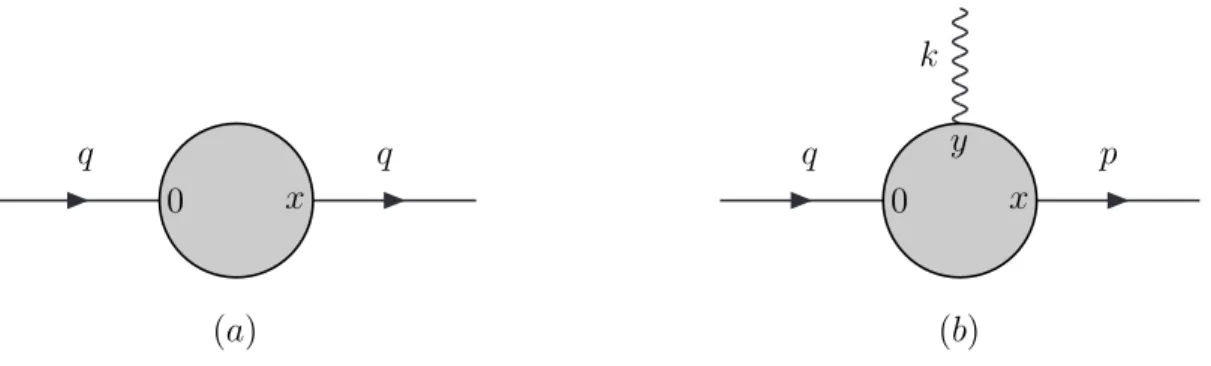
(a)

q q

0 x

(b)

q p

k

0 x

y

Figure 2.1: Representation of (a) the two-point and (b) the three-point correlation functions.

moments and others. Besides, one has by construction a physical model that

simultane-ously considers the non-perturbative effects of QCD vacuum at low energies and also all

the theoretical information from the QCD perturbative at high energies. However, there

are some limitations on the accuracy of the QCDSR due to the approximations made

in the correlation function on both sides of the approach: QCD and Phenomenological

side. Therefore, each sum rule must be carefully studied in order to verify its region of

applicability.

Through the following sections, one discuss in more detail the most relevant properties

of QCDSR to the present work, identifying the necessary steps for calculate the hadron

masses.

2.1 Correlation Function

In sum rules, the correlation function is defined as the functional expectation value

of a time-ordered product of n-field operators at different positions. Particularly, the

two-point correlation function, which contains the time-ordered product of two hadronic

currents, is useful to estimate the hadron masses and decay constants. It is related to the

amplitude of Fig.(2.1a) and can be evaluated through the expression:

Π(q) =i

%

(39)

2.1. CORRELATION FUNCTION 17

where q is the total four-momentum andj(x) is the hadronic current determined by the

quantum numbers and by the appropriate quark content in the structure of the hadron

to be studied.

The calculation of the form factors and decay widths of a vertex interaction between

three scalar particlesX,Y andZ is done using the three-point correlation function shown

in Fig.(2.1b) and whose expression is given by

Φ(q, k, p) =

%

d4x

%

d4y eip·x eik·y_!0|T[jX(x)jY(y)j

†

Z(0)]|0" , (2.2)

wherepand k are the loop four-momenta leaving the diagram, respectively, at the points

x and y. This expression is quite useful to study the decay channels such as Z _→X Y.

Since Eqs.(2.1) and (2.2) could be used to study vector hadrons, one should separately

analyze the Lorentz structures present in the correlation functions of both mesons and

baryons.

For vector mesons described by a conserved current jµ(x), the Lorentz structures of

the correlation function to be considered are:

Πµν(q) =i %

d4x eiq·x _!0|T[jµ(x)jν†(0)]|0" =−

&

gµν −

qµqν

q2 '

Π1(q2) (2.3)

whereΠ1(q2) is an invariant function and must contain the appropriate quantum numbers

of the vector meson. The conservation of the current implies that the correlation function

(2.3) has only a transversal component in its structure. On the other hand, if the current

is not conserved, one longitudinal component associated with a scalar state emerges, so

that:

Πµν(q) =− &

gµν −

qµqν

q2 '

Π1(q2) +

qµqν

q2 Π0(q

2₎ _(2.4)

(40)

respec-tively the quantum numbers of the vector and scalar state. Once the complete expression

of Πµν(q) is calculated, it is possible to determine the two invariant functions using the

following expressions:

Π1(q2) = −

1 3

&

gµν₋ q

µ_qν

q2 '

Πµν(q) (2.5)

Π0(q2) =

qµ_qν

q2 Πµν(q) . (2.6)

Therefore, the two-point correlation function described by a non-conserved current allows

to estimate the mass and decay constant of two states at the same time, one vector and

other scalar state.

For the spin 1/2+ _{and 3}_/₂+ _{baryons, the expressions are respectively given by}

Π1/2₍_q_{) =} _/qF

1(q2) +F2(q2) , (2.7)

Π3/2µν(q) = gµν (

/qF1(q2) +F2(q2) )

+· · · , (2.8)

where one must calculate both invariant functions F1(q2) and F2(q2). In the case of spin

3/2+ _{baryons, many works in sum rules [73] demonstrate that the structure} _g

µν of the

correlation function is enough for providing information of the ground-state baryons.

As previously discussed, in QCDSR the correlation function can be described in two

ways. In the QCD side, one calculates the correlation function with the appropriate

hadronic current in terms of the quark and gluon fields and the condensates. In the

Phenomenological side, one calculates it using experimental data, such as masses and

decay constants, and parameterize the strength of the coupling between the current and

all states of the hadron. Finally, the results for both descriptions can be compared in

(41)

2.2. LOCAL OPERATOR PRODUCT EXPANSION 19

2.2 Local Operator Product Expansion

In the QCD side, the calculation of the correlation function is based on the Local

Operator Product Expansion (OPE) of the quark and gluon fields. This technique was

introduced by K.G. Wilson in Ref. [74], where the OPE would describe analytically the

complex structure of the QCD vacuum. Its application to the correlation function (2.1)

is done in such a way that

i

%

d4x eiq·x _!0|T[j(x)j†(0)]|0_" = *

d

Cd(q2)!0|Oˆd(0)|0" (2.9)

where the coefficientsCd(q2) are the so-called Wilson coefficients, which contain the effects

of the QCD perturbative, at high energies. The vacuum expectation values (VEV) of the

local operators ˆOd(0) parameterize the non-perturbative effects of the QCD vacuum in

terms of the condensates. The d-index represents the dimension of the local operator.

In QCDSR, the dimension-zero operator is given by ˆO0 = ˆ1 and the coefficient C0(q2)

represents the contributions from the QCD perturbative. Considering only the lowest

dimension local operators in the OPE, one obtains:

ˆ

O3 = : ¯q(0)q(0) : ≡ qq¯

ˆ

O4 = :g2sGNαβ(0)GNαβ(0) : ≡ gs2G2

ˆ

O5 = : ¯q(0)gsσαβGNαβ(0)q(0) : ≡ qGq¯

ˆ

Oq₆ = : ¯q(0)q(0) ¯q(0)q(0) : _≡ qq¯ qq¯ ˆ

OG₆ = :fNM Kg

3

sGNαβ(0)GMβγ(0)GKγα(0) : ≡ gs3G3 (2.10)

where the symbol :: represents the normal ordering of the operators, q(0) is the quark

field, GN

αβ(0) is the gluon field tensor, fNM K is the structure constant of the SU(3) group

and σαβ = ₂i [γα,γβ]. The VEV of these local operators

(42)

gives rise to expressions for the quark condensate _!qq¯ _", gluon condensate _!g2

sG2", mixed

condensate _!qGq¯ _", four-quark condensate _!qq¯ qq¯ _" and the triple gluon condensate _!g3

sG3".

In general, considering the contributions up to dimension-six is enough for calculating the

hadronic parameters. Discussions on the condensates of higher dimension (d > 6), the

difficulties to introduce them properly into the QCDSR and also their relevance to the

OPE convergence can be found in Refs. [19, 75, 76].

The Wilson’s OPE is useful to transform non-local operators,qa(x) ¯qb(0), into a sum of

local operators ˆOd, whose vacuum expectation values form the condensates. One obtains

the main contributions when considering only the light quark field operators (q =u, d, s).

In general, the contributions of the condensates formed by heavy quark field operators:

!QQ¯ _", _!QGQ¯ _", . . . are negligible and do not contribute to the QCDSR. However, the

relevance of these condensates should be studied carefully, especially in cases where the

light quark condensates are missing in hadronic structure, which make them the principal

source of non-perturbative effects of QCD vacuum. By convention, hereafter the quark

field operators qa(x) stand for light quarks andQa(x) stand for heavy quarks.

One uses the Eq.(2.9) to calculate the contribution of leading order contributions to the

OPE. However, it is possible to rewrite it in a more general form, where the contributions

of the radiative corrections in the OPE can be introduced. For this purpose, one should

consider the following equation for the correlation function, in the QCD side [77]:

Π(q) =i

%

d4x eiq·x _!0|T[j(x)j†(0) ei!d4yLint(y)]|0" (2.12)

where the interaction Lagrangian between quarks and gluonsLint is given by

L_int(y) = tN

cdgsq¯c(y)γαANα(y)qd(y) , (2.13)

the latin indices (a, b, c, . . .) represent the color charge of quark and gluon fields, the greek

indices (α,β,γ, . . .) represent the spinorial indices, tN

(43)

is the QCD strong coupling constant, γα _{are the Dirac matrices,} _AN

α(y) the gluon fields

and N = (1, . . . ,8) are the SU(3) group generators. Expanding in series the exponential

term contained in the VEV of Eq.(2.12), one obtains

Π(q) = ∞

*

n=0

in+1

n!

%

d4x0d4x1. . . d4xn eiq·x0 !0|T[j(x0)j†(0)Lint(x1). . .Lint(xn)]|0"(2.14)

Explicitly, the first terms of this expansion are given by

Π(q) = i

%

d4x eiq·x

+

!0|T[j(x)j†_(0)]_|₀

"+i

%

d4y _!0|T[j(x)j†₍₀₎_L

int(y)]|0"

−1₂

% %

d4y d4z _!0|T[j(x)j†₍₀₎_L

int(y)Lint(z)]|0" + . . .

,

≡ i

%

d4x eiq·x

+

Π(0)(x) +Π(1)(x) +Π(2)(x) +. . .

,

, (2.15)

where the definition of Π(n)(x) functions is settled. As expected, Eq.(2.1) is the leading order term of the expansion (2.15). The other terms include the non-perturbative

contri-butions from the higher dimension condensates in the OPE and the radiative corrections

up toO(g2

s), as well. To illustrate how the correlation function (2.15) is written in terms

of the OPE, consider the scalar current: j(x) = ¯qa(x)qa(x). Inserting into the VEV of

the first term of the expansion (2.15), one obtains the time-ordered product of four quark

fields. Applying Wick’s theorem, this may be expressed as:

Π(0)(x) = _!0|T [¯qa,i(x)qa,i(x)¯qb,j(0)qb,j(0)]|0"

= _{− !}0p|T [qa,i(x)¯qb,j(0)]|0p" !0p|T[qb,j(0)¯qa,i(x)]|0p" +

− !0p|T [qb,j(0)¯qa,i(x)]|0p" !0|:qa,i(x)¯qb,j(0) : |0" +

− !0p|T [qa,i(x)¯qb,j(0)]|0p" !0|:qb,j(0)¯qa,i(x) :|0" +

+ _!0|: ¯qa,i(x)qa,i(x)¯qb,j(0)qb,j(0) :|0"

= ₋Tr#

S_ab0(x)S_ba0 (₋x)$

−Tr#

S_abqq¯(x)S_ba0 (₋x)$

−Tr#

S_ab0 (x)S_baqq¯(₋x)$

(44)

Figure 2.2: Diagrams related to the Π(0)₍_x_{) function of the scalar current,}_j₍_x_{) = ¯}_q

a(x)qa(x), where the first diagram is the perturbative contribution and the other diagrams represent the non-perturbative

effects from the QCD vacuum. The gray blobs give rise to the condensates formed by the VEV of the

quark fields: !0|:qa(x)¯qb(0) :|0".

where . . . represents terms which are proportional to the higher order condensates (e.g.

the four-quark condensate_!qq¯ qq¯ _"contribution). From now on, these kinds of contributions

will be omitted. The notation |0p"represents the perturbative vacuum and|0" represents

the physical QCD vacuum, S0

ab(x) is the perturbative propagator for free quarks defined

as:

Sab0(x) = iδab

% _d4_p

(2π)4 &

/p+mq

p2₋_m2 q+i$

'

e−ip·x (2.17)

and S_abqq¯(x) is the non-perturbative correction to the quark propagator and its expression is given by

S_abqq¯(x) = _!0|:qa(x)¯qb(0) : |0" . (2.18)

For each trace in Eq.(2.16), one has corresponding diagrams represented in Fig.(2.2). If

the QCD vacuum could be treated perturbatively, the VEVs of normal ordering of quark

fields in Eq.(2.16) would be zero and the time-ordered products of fields would be reduced

to the usual perturbative propagators of the quantum field theory. However, the fact that

the contributions of these VEVs are not zero introduces non-perturbative effects from the

QCD vacuum to the sum rules.

Similarly, one does the same calculation for the other terms of the expansion (2.15).

(45)

Figure 2.3: Diagrams related to the Π(1)₍_x_{) function of the scalar current} _j₍_x_{) = ¯}_q

a(x)qa(x), where

the gray blobs represent the non-perturbative effects from the QCD vacuum, linked to the condensates

formed by the VEV of the quark and gluon fields: !0|:qa(x)¯qb(0) :|0".

(2.13), one obtains the following expression for the Π(1)₍_x_):

Π(1)(x) = i tN

cd %

d4y_!0|T #

¯

qa(x)qa(x) ¯qb(0)qb(0) ¯qc(y)γαgsAαN(y)qd(y) $

|0_"

= ₋i tN

cd %

d4y

-Tr#

Sbc0(−y)γαSda0 (y−x)!0|:qa(x)gsAαN(y)¯qb(0) :|0" $

+

+ Tr#

S_ac0 (x₋y)γαS_db0 (y)_!0|: ¯qa(x)gsAαN(y)qb(0) :|0" $

.

(2.19)

note that any other contraction of quark fields results in disconnected diagrams and,

therefore, do not contribute to Π(1)(x).

For the gluon field AN

α(y), contained within the VEV of Eq.(2.19), it is convenient to

work with the fixed-point gauge or the Fock-Schwinger gauge [78]:

yα_AN

α(y) = 0 . (2.20)

so that, at the low-energy regime, it is possible to approximate the gluon field AN

α(y) in

terms of the totally antisymmetric gluon field strength tensor :

ANα(y)≃ −

1 2 G

N

αβ(0)y

β

. (2.21)

(46)

the Fock-Schwinger gauge as:

Π(1)(x) = i t

N

cd

2

%

d4y

-Tr#

S_bc0(₋y)γαyβ _S0

da(y−x)!0|:qa(x)gsGNαβ(0)¯qb(0) :|0" $

+

+ Tr#

S_ac0 (x₋y)γαyβS_db0 (y)_!0|: ¯qa(x)gsGNαβ(0)qb(0) :|0" $

.

= Tr

(

SqqG¯ Nαβ

ab (x)S Gαβ_N ba (−x)

)

+ Tr

(

SGαβN

ab (x)S qqG¯ N

αβ

ba (−x) )

(2.22)

where the following definitions are introduced:

SG αβ

N

ab (x) =

i tN

cd

2

%

d4y S_ac0 (x₋y)γαyβS_db0 (y) (2.23)

SqqG¯ Nαβ

ab (x) = !0|: ¯qa(x)gsGNαβ(0)qb(0) :|0" (2.24)

Observe that Eq.(2.23) is associated with the quark propagation through space and, in a

certain point, it emits a non-perturbative gluon, Gαβ_N . Since, this gluon field is defined in

the Fock-Schwinger gauge, hence the label “non-perturbative gluon”. In turn, Eq.(2.24)

receives this emitted gluon forming the condensate from the VEV of the quark and gluon

fields. The diagrams are represented in Fig.(2.3), where they are associated to each trace

in Eq.(2.22)

Finally, one calculates the Π(2)₍_x_{) function of the expansion (2.15). Then:}

Π(2)(x) = ₋t

N cdtMef

2

% %

d4y d4z_!0|T#

¯

qa(x)qa(x) ¯qb(0)qb(0) ¯qc(y)

× γαgsANα(y)qd(y)¯qe(z)γβgsAβM(z)qf(z)

$

|0_"

= t

N cdtMef

2

% %

d4y d4z g_s2_!0|T #

ANα(y)AMβ (z) $

|0_"

×

-Tr#

S0

ba(−x)Sae0 (x−z)γβSf c0 (z−y)γαSdb0 (y) $

+ Tr#

S_ab0(x)S_bc0(₋y)γαS_de0 (y₋z)γβ S_{f a}0 (z₋x)$

+ Tr#

S_be0(₋z)γβ S_{f a}0 (z₋x)S_ac0 (x₋y)γαS_db0 (y)$ .

(47)

Figure 2.4: Diagrams related to the Π(2)₍_x_{) function of the scalar current}_j₍_x_{) = ¯}_q

a(x)qa(x). The first

three diagrams provide the NLO contributions, given by theΠ(2)N LOfunction. The last ones, which contain

the gray blobs, provide the non-perturbative effects from the QCD vacuum, related to the condensates

formed by the VEV of the gluon fields: !0|:g2

sGNαρ(0)GMβλ(0) :|0".

Using the definition of the time-ordered product of the gluon fields, one can deduce:

g2_s_!0|T #

AN_α(y)AM_β (z)$

|0_" = g_s2_!0p|T#ANα(y)A

M

β (z)

$

|0p"+!0|:gs2ANα(y)A

M

β (z) :|0"

≡ δN M gs2SαβGG(y−z) +

yρ_zλ

4 !0|:g

2

sGNαρ(0)GMβλ(0) :|0" (2.26)

Note that the expression SGG

αβ (y−z) is the perturbative gluon propagator, which is well

defined in the coordinate space and the Feynman gauge, so that:

SαβGG(y−z) = −i %

d4p

(2π)4 &

gαβ

p2 ₊_i_$ '

e−ip·(y−z) . (2.27)

Therefore, the VEV in Eq.(2.26) contains the non-perturbative contributions of the gluon

fields and, for this reason, it should be expressed in the Fock-Schwinger gauge (2.20).

Inserting the definition (2.26) into Eq.(2.25), one obtains:

Π(2)(x) = Π(2)N LO(x) + Tr /

S_ab%G2&(x)Sba0 (−x) 0

+ Tr/Sab0(x)S

%G2_&

ba (−x) 0

+ 1 2!0|:g

2

sGNαρ(0)GMβλ(0) :|0"Tr (

SG αρ

N

ab (x)S Gβλ_M ba (−x)

)

(48)

where the definition of the non-perturbative correction to the gluon propagator was

in-troduced and is given by

S_ab%G2&(x) = t

N cdtMef

8 !0|:g

2

sGNαρ(0)GMβλ(0) :|0"

×

% %

d4_{y d}4_{z y}ρ_zλ _S0

ae(x−z)γβSf c0 (z−y)γαSdb0 (y) . (2.29)

For simplicity, the Π(2)N LO(x) function associated with the radiative corrections is not

ex-pressed explicitly in Eq.(2.25) since, in the present work, the sum rules will be only

evaluated with the leading order term in αs. The diagrams, related to each term of

Eq.(2.25), are shown in Fig.(2.4).

In quantum field theory, the calculation of a general fermion loop diagrams corresponds

to evaluating traces of these fermion propagators. Then, notice that theΠ(n)(x) functions, given by Eqs.(2.16), (2.22) and (2.25), contain exactly the traces of the perturbative

propagators as well as the non-perturbative propagators obtained from the VEVs. In

general, it is possible to demonstrate that, for any hadronic currentj(x) used in QCDSR,

the expression for Π(n)(x) function is always the same. Therefore, now it is convenient to introduce the definition of the full propagator of QCD, given by

SQCD₍_x_{) =} _S0

ab+SαβGG(x) +S qq¯

ab(x) +S Gαβ_N

ab (x) +S qqG¯ N

αβ

ab (x) +S

%G2_&

ab (x) , (2.30)

where each term of this propagator gives the most relevant diagrams for a QCDSR

cal-culation.

A detailed analysis of the calculation of the full propagator of QCD is presented in

Appendix B. In summary, the expressions of non-perturbative light quark propagators,

in the coordinate space, are given by

S_abqq¯(x) = ₋δab

12 !qq¯ "+

iδabx/

48 mq!qq¯ " −

δabx2

192 !qGq¯ "+

iδabx2x/

(49)

SG αβ

N

ab (x) = −

i tN ab

32π2_x2 (σαβ x/+x/σαβ) +. . . (2.32)

SqqG¯ Nαβ

ab (x) = −

tN abσαβ

192 !qGq¯ " −

i tN ab

768(σαβ /x+x/σαβ)mq!qGq¯ "+. . . (2.33)

S_ab%G2&(x) _≃ 0 . (2.34)

In the case of non-perturbative heavy quark propagators, the heavy quark condensate

contribution _!QQ¯ _" and the heavy mixed condensate_!QGQ¯ _" are given by [79]:

!QQ¯ _{" ≃ −} 1

48π2 _m Q !

g_s2G2_" (2.35)

!QGQ¯ _{" ≃ −} 5

96π2 _m Q !

g_s3G3_". (2.36)

As one can see, both condensate contributions are suppressed by the presence of the

heavy quark mass, mQ, in the denominator of Eqs.(2.35) and (2.36), in such a way these

contributions can be neglected during the calculation of the full propagator of QCD for

heavy quarks. Therefore, the most relevant non-perturbative contribution involving heavy

quarks comes from the gluon condensate (2.34). The expressions of the non-perturbative

heavy quark propagators, in the momentum space, are given by

S_abQQ¯(p) _≃ 0 (2.37)

SG αβ

N

ab (p) = −

i tN ab

4(p2₋_m2 Q)2

#

σαβ(/p+mQ) + (/p+mQ)σαβ $

(2.38)

SQQG¯ Nαβ

ab (p) ≃ 0 (2.39)

S_ab%G2&(x) = iδabmQ 12(p2₋_m2

Q)3 1

1 + mQ(/p+mQ)

p2₋_m2 Q

2

(50)

2.3 QCD Side

After choosing the hadronic current of interest, evaluating the OPE up to desired

dimension and working with the most relevant condensates in the sum rules the next step

is to express the correlation function (2.1) in terms of a dispersion relation:

ΠOP E₍_q_{) =}

+∞

%

tq ds ρ

OP E₍_s₎

s₋q2 (2.41)

where tq is a kinematic limit, which usually corresponds to the square of the sum of the

current quark masses of the hadron. The OPE spectral density, ρOP E₍_s_{), is defined in such}

a way the perturbative and condensate contributions are inserted through the following

relation:

ρOP E₍_s_{) =} _K

0(s) + K3(s)!qq¯ " + K4(s)!gs2G2" + K5(s)!qGq¯ " + . . . (2.42)

where:

Kd(s)≡

1

πIm[Cd(q

2_)] _. _(2.43)

There are some advantages of expressing the correlation function in terms of a dispersion

relation. With that, one can do a better comparison between the QCD side and

Phe-nomenological side of the sum rules and separate the ground-state contribution from the

one related to the continuum.

2.4 Phenomenological Side

In the Phenomenological side, the correlation function (2.1) is evaluated in terms

of hadronic parameters and the current is interpreted as the creation and annihilation

(51)

2.4. PHENOMENOLOGICAL SIDE 29

rewrite the correlation function as:

Π(q) =i

%

d4x eiq·x 3

!0|θ(x0)j(x)j†(0)|0" + !0|θ(−x0)j†(0)j(x)|0"

4

(2.44)

Once more, for simplicity, one considers the scalar current j(x) = ¯qa(x)qa(x). Assuming

that the hadrons H(p)_≡Hp created by the current j(x) form a complete set of hadronic

states, so it is possible to use an unitary projector through the completeness relation of

these states:

*

Hp

1 (2π)3

%

d3_p_.

2p0

|Hp "!Hp|= ˆ1, (2.45)

where the sum evolves the ground-state hadron and all its resonant states. Introducing

this projector between the currentsj(x) andj†_{(0) in both terms of Eq.(2.44), one obtains:}

Π(q) = i

%

d4x eiq·x *

Hp

%

d3_._p

(2π)3₂_p 0

(

θ(x0)!0|j(x)|Hp"!Hp|j†(0)|0"

+ θ(₋x0)!0|j†(0)|Hp"!Hp|j(x)|0"

)

(2.46)

Expressing the current j(x) in terms of a translation operator, ˆU =ei_p_·_x_{, one gets:}

j(x) =eip·x j(0) e−ip·x (2.47)

Inserting into Eq.(2.46) the correlation function becomes:

Π(q) = i

%

d4x eiq·x *

Hp

%

d3_._p

(2π)3₂_p 0

(

!0|j(0)|Hp"!Hp|j†(0)|0"θ(x0) e−ip·x

+ _!0|j†₍₀₎_|_H

p"!Hp|j(0)|0"θ(−x0)eip·x

)

= i

%

d4x eiq·x *

Hp

% _d3_._p

(2π)3₂_p 0

(

θ(x0) e−ip·x+θ(−x0) eip·x )

(52)

Notice that it is possible to identify the Feynman propagator in Eq.(2.48):

∆F(x) = %

d3_._p

(2π)3₂_p 0

(

θ(x0)e−ip·x+θ(−x0) eip·x )

= i

%

d4_p

(2π)4

e−ip·x

p2₋_E2 H +i$

(2.49)

where EH is the energy associated with the|Hp" state. Therefore, one gets

Π(q) = ₋

%

d4x eiq·x *

Hp

%

d4_p

(2π)4

e−ip·x

p2 ₋_E2 H +i$

|_!0|j(0)|Hp"|2 . (2.50)

Introducing the following identity into the Eq.(2.50),

+∞

%

0

ds δ(s₋E_H2) = 1 , (2.51)

where the integral is well defined on the entire spectrum of the hadron H, one finally

obtains the result:

Π(q) = ₋

+∞

%

0

ds

%

d4x eiq·x *

Hp

%

d4_p

(2π)4

e−ip·x

p2 ₋_s₊_i_$|!0|j(0)|Hp"|

2

δ(s₋E_H2)

= ₋ +∞ % 0 ds * Hp %

d4p 1

p2₋_s₊_i_$|!0|j(0)|Hp"|

2

δ(s₋E_H2) δ(q₋p)

=

+∞

%

0

ds 1

s₋q2₋_i_$ *

Hq

|_!0|j(0)|Hq"|2δ(s−EH2)

≡

+∞

%

0

ds ρ(s)

s₋q2₋_i_$ (2.52)

which contains the definition for the spectral density:

ρ(s) = *

Hq

Estados Exóticos do Charmonium

!

THESE!de!DOCTORAT!!

Raphael!Moreira!de!ALBUQUERQUE!

ETATS!EXOTIQUES!DU!CHARMONIUM!

Universidade de S˜

ao Paulo

Instituto de F´ısica

Estados Ex´

oticos do Charmonium

Raphael Moreira de Albuquerque

S˜

ao Paulo, 2012

FICHA CATALOGRÁFICA

Preparada pelo Serviço de Biblioteca e

Informação

do Instituto de Física da Universidade de São

Paulo











Contents

Chapter 1

Introduction

1.1

Charmonium Exotic States

1.1.1

Y(4260), Y(4360) and Y(4660)

1.1.2

Y

(4140)

1.1.3

Y(3930)

0

2

4

6

8

4.2

4.4

4.6

4.8

5

M(

φ

J/

ψ

) (GeV/c

)

Entries/25 MeV/c

1.1.4

X(4350)

1.1.5

Y

(10890)

1.2

B

Meson Spectroscopy

1.3

Heavy Baryons in QCD

1.3.1

Baryons with One Heavy Quark

(

Qqq

)

1.3.2

Baryons with Two Heavy Quarks

(

QQq

)

Chapter 2

QCD Sum Rules

2.1

Correlation Function

2.2

Local Operator Product Expansion

2.3

QCD Side