Critical Behavior of a Bounded Kardar-Parisi-Zhang Equation
Miguel A. Mu˜noz,
Departamento de Electromagnetismo y F´ısica de la Materia, Universidad de Granada, Fuentenueva s/n, 18071 Granada, Spain
Francisco de los Santos,
Center for Polymer Studies and Department of Physics, Boston University, Boston, MA 02215, USA
and Abdelfattah Achahbar
Departement de Physique, Facult´e des Sci`ences, B.P. 2121 M’hannech, 93002 Tetouan, Morocco
Received on 1st April, 2003
A host of spatially extended systems, both in physics and in other disciplines, are well described at a coarse-grained scale by a Langevin equation with multiplicative-noise. Such systems may exhibit nonequilibrium phase transitions, which can be classified into universality classes. Here we study in detail one such class that can be mapped into a Kardar-Parisi-Zhang (KPZ) interface equation with a positive (negative) non-linearity in the presence of a bounding lower (upper) wall. The wall limits the possible values taken by the height variable, introducing a lower (upper) cut-off, and induces a phase transition between a pinned (active) and a depinned (absorbing) phase. This transition is studied here using mean field and field theoretical arguments, as well as from a numerical point of view. Its main properties and critical features, as well as some challenging theoretical difficulties, are reported. The differences with other multiplicative noise and bounded-KPZ universality classes are stressed, and the effects caused by the introduction of “attractive” walls, relevant in some physical contexts, are also analyzed.
I
Introduction
Nonequilibrium phase transitions occurring in systems amenable to be described by Langevin equations including a multiplicative noise (MN) term are the subject of current intense studies. This embraces a broad variety of systems both in physics and in other disciplines. A phenomenology much richer and complex than that appearing in equilibrium systems, including counterintuitive behaviors, has been re-ported to appear in these, typically nonequilibrium, situa-tions. See [1,2] for detailed introductions to this growing field, including many different realizations.
The interest in MN problems is enlarged even further, because of the existing mappings between them and other prototypical nonequilibrium problems [2]. A well known in-stance is the Kardar-Parisi-Zhang (KPZ) equation, describ-ing the kinetic roughendescrib-ing transition of generic interfaces under nonequilibrium conditions [3, 5, 4], which can be mapped onto a MN Langevin equation, by performing the so called Cole-Hopf transformation linking the interface height at each point with the activity field of the MN equation. If an interface under consideration is described by the KPZ equa-tion and it is physically limited by a wall,i.e. if the heights cannot be larger or smaller than a certain value, then this problem,bounded KPZ, can be mapped into a multiplicative noise equation by employing the abovementioned transfor-mation [2,6,7]. The bounded KPZ equation may experience,
as parameters are varied, a phase transition from a depinned phase in which the interface escapes with probability one from the wall, to a pinned phase characterized by a finite ex-pectation value of the stationary averaged height (measured from the wall). In the MN language (i.e. after employing the Cole-Hopf transformation) the pinning-depinning transi-tion corresponds to a critical point separating anabsorbing phasein which the order parameter goes exponentially to zero (depinned phase) to anactive phasein which the order parameter takes a nonvanishing average value.
Surprisingly enough, it was shown a few years ago that the introduction of “upper” or “lower” walls into a given KPZ equation (with a fixed non-linearity sign) lead to quite different phenomenologies. The origin of this can be tracked down to the fact that the KPZ equation is not invariant upon inverting the height (see [8] or [2] for a more detailed expla-nation). Taking, for instance, the sign of the coefficient of the KPZ non-linearity to be positive, the introduction of an upper wall leads to a (well established by now) set of critical exponents characterizing the so called multiplicative noise 1 (MN1) universality class [6-9]. On the other hand, a wall limiting negative values of the interface height (lower wall) leads to a different type of phase transition as shown by T. Hwa and one of us some years back [8]. In what follows, and following the nomenclature introduced in [2], we will use the term MN2 to denote this class.
non-linearity and a lower wall is completely equivalent to a KPZ with a negative non-linearity coefficient and an up-per wall [2]: one just has to change the sign of the height variable in the KPZ-like equation to verify this.
The MN2 class is of great importance in the context of alignment of DNA and other biological sequences. It has been argued by Hwa and collaborators, that the phase tran-sition appearing upon changing the so called scoring pa-rameter in the commonly used alignment algorithm can be mapped into the MN2 critical point [14]. It is also related to some instances of nonequilibrium wetting [10]. For some other applications and physical instances within this class see [2] and references therein.
While the MN1 class has been extensively studied, es-pecially after its connections with nonequilibrium wetting [10-12] and with the problem of synchronization in ex-tended systems were established [2, 13], the MN2 class re-mains poorly studied. Furthermore, recent numerical analy-ses have revealed that the preliminary critical exponent val-ues reported in [14] might be far from their true asymptotic values.
Aimed at clarifying these issues, it is the purpose of this paper to analyze the MN2 phase transition in one di-mensional systems using: i) mean-field and field-theoretical techniques and ii) numerical (Monte Carlo) analysis of dif-ferent models claimed to belong to this class.
Finally let us stress that if the wall becomes attractive, rather than simply bounding, new phenomenology might ap-pear. This is particularly interesting in the context of syn-chronization [2, 13]. This possibility will also be discussed in the paper.
II
The MN2 class
Let us consider a KPZ equation with a positive non-linearity coefficient,λ >0, in the presence of a lower wall,
∂th(x, t) =a+b e−ph+D∇2h+λ(∇h)2+ση(x, t). (1)
wherehis a height variable, a represents a constant drift whileb e−ph
is a bounding wall. The parameterp >0 con-trols the wall penetrability, the limitp→ ∞corresponding to a perfectly rigid (impenetrable) wall. It has been shown previously that for both the MN1 and the MN2 classes the magnitude of pdoes not influence the asymptotic proper-ties at criticality [6, 7] (its sign, however, is important, as it determines whether the wall is a lower or an upper one). The same property applies to equilibrium systems (i.e., for
λ= 0) [15].ηis a stochastic white noise withhηi= 0and
hη(x, t)η(x′
, t′
)i= 2δ(t−t′
)δ(x−x′
), whereh·idenotes an average over the distribution of the noise.
For a fixed value ofbthe interface experiences a pinning-depinning transition at some valuea=ac.
Some remarks concerning the connection of the previ-ous equation with wetting problems follow. Whenh(x, t)is viewed as the distance separating a liquid-gas interface from a solid wall, Eq. (1) can then be interpreted as a dynamic model for nonequilibrium wetting. Under this perspectivea
is the chemical potential difference between the liquid and
the gas phases,hhiis the thickness of the wetting layer, and the wall is a, physical substrate. Atbulk phase coexistence, i.e. for the value ofa=ac for which in the absence of the
wall the interface does not move on average, hhidiverges at all temperatures above certain wetting temperature,TW,
while for a 6= ac the thickness of the liquid film can be
big, but finite (pinned interface). The temperature here is controlled by the parameterb, which vanishes linearly with the mean-field wetting temperature asT −TW. Thus, on
approaching coexistence forT > TW (b > 0at the
mean-field level),hhidiverges ashhi ∼ |a−ac|βh. This transition,
termedcomplete wetting, is always continuous and the value of theβh exponent depends on the nature of the forces
be-tween the particles in the fluid phases and the wall. In this paper only short-range, exponentially decaying interactions between all the particles and the substrate (as described by Eq. (1)) are considered.
The change of variablesn = exp(−h)transforms Eq. (1) into the MN2 Langevin equation:
∂tn(x, t) =∇2n−2
(∇n)2
n −(a+ 1)n−bn
p+1+nη, (2)
where for the sake of simplicity we have setλ=D=σ= 1
and Ito calculus [16] has been used (different coefficients for the Laplacian and the KPZ non-linear term could be reabsorbed using n = exp(−αh)with a proper choice of
α). This transformation maps the depinning from the wall
hhi → ∞to a transition into an absorbing statehni → 0. The physical equivalence between the casesλ > 0with a lower-wall (p >0), andλ < 0with an upper wall (p <0), reflects in the fact that the same equation is obtained using
n= exp(−h)andn= exph, respectively.
Observe that Eq.(2) is identical to the MN equation de-scribing the MN1 class [2, 6, 7], except for the presence of an extra term (∇n)2/n. This term can also be written as
(∇n)·(∇ln(n)) = (∇n)·(∇h)suggesting that the inter-face language is the natural one for this class. In fact, except for the factor 2 in front of(∇n)2/nEq. (2) coincides with
the Cole-Hopf transform of
∂th(x, t) =∇2h+a+be−ph+η(x, t) (3)
that describes the growth of wetting layers toward their equi-librium state [19] (observe that this is just the equiequi-librium, Edwards-Wilkinson model, in the presence of a bounding wall). Note also that the factor2in Eq. (2) cannot be read-sorbed by reparametrizing.
Finally, let us underline that in the regime whereb < 0
the wall becomes attractive (which might be necessary to describe some physical situations as, for instance, synchro-nization problems as said in the introduction) and a new term, say,cexp(−2h)(equivalentlycn2p+1) withc >0has
to be added to stabilize the equation.
III
Mean-field approaches
Mean-field approaches to Eq. (1) can be implemented with several degrees of sophistication. A crude approximation consists of ignoring the noise and spatial variations. At this level one trivially gets that the order parameterhhivanishes as a → 0 with an exponent βh = 0. When applied to
Eq.(2), this approximation yields a shifted critical point at
ac =−1and the usual result for the order parameter critical
exponent,βn = 1/p. But, as experience with other systems
with multiplicative-noise dictates, neglecting completely the noise is a too crude approximation, that eliminates most of the characteristic traits of MN physics.
Now the effect of allowing a spatially varying order
pa-rameter and taking the noise into consideration are exam-ined. The Laplacian is discretized as
∇2n
i=
1 2d
X
j
(nj−ni)≈ hni −ni, (4)
where the sum runs over the nearest neighbors ofi and a large system dimensionality has been assumed. Similarly, the square gradient term can be written as
(∇n)2
i
ni
≈ hn
2i ni
−2hni+ni. (5)
The one-site stationary probability distribution is then read-ily obtained from the associated Fokker-Planck equation,
⌋
Pst
³
n,hni´ ∝ 1
n2exp
Z n(∇x)2
i −2(∇x)2i/xi−(a+ 1)xi−bxpi+1
x2
i
dxi,
≈ 1
na+6exp Ã
−5hni
n −b np
p +
hn2i n2
!
. (6)
⌈
wherehniandhn2ihave to be calculated self-consistently.
Fora < ac = −5,Pst is not normalizable, which means
that the stationary state is the absorbing phasehni= 0. For
hni 6= 0, however, the non-analyticity of exp[hn2i/n2] at n = 0 again renders Pst non-normalizable. As a result,
there is no well-defined active phase at this mean-field level for Eq. (6). Similar problems are found if the same type of approach is applied to Eq. (1) instead of Eq. (2).
To avoid the presence of the square gradient term in Eq. (2), and the complications of its, somewhat arbitrary, dis-cretization, we resort to a different change of variables. Af-tern= exph,
∂tn = ∇2n+ (a+ 1)n+bn3−p+nη,
Pst ∼
1
n2−aexp
·bn2−p
2−p −
hni
n ¸
. (7)
These equations are simpler than (2) and (6), but at the cost thathniis no longer an order parameter as, at the transition pointhni → ∞rather than going to0. Furthermore, Lan-dau expansions only make sense when the order parameter vanishes at the critical point, making the whole approach in-consistent. One possible way to circumvent this problem is to monitor m ≡ 1/n, and studyP˜st(m)dm = Pst(n)dn,
but given the non-Gaussian nature of the probability distri-bution the substitutionhni= 1/hmiis likely to be incorrect, and there seem to be no safe way to proceed.
Summing up, non-trivial mean-field approaches detect some problems with the model under consideration, and are not able to predict a phase correct phase diagram. A sound mean-field approximation therefore needs to be found. No-tice that none of these problems occur in the case of a nega-tive KPZ non-linearity,i.e. in the MN1 class, where a
stan-dard mean-field approximation yields qualitatively correct results (see [2, 12] and references therein).
IV
Field theoretical considerations
The Langevin equation for MN1 is known to be super-renormalizable,i.e. Feynman diagrams can be computed to all orders and resummed. This does not imply that critical exponents can be computed in all the cases, as the renormal-ization group flow-equation has runaway trajectories sup-posed to converge to astrong coupling fixed point. But at least, the correct phase diagram, including strong and weak coupling fixed points can be obtained.
For the MN2 the situation is far more complicated, as can bea priorianticipated given the failure of mean-field approaches. The extra term,(∇n)2/n, being singular inn
V
Numerical results
Owing to the failure of standard (nontrivial) mean-field ap-proaches and lacking so far an alternative analytical route, numerical methods are required to glean insight into the sys-tem properties. We have carried out simulations of two sur-face growth models. Both of them, in the absence of walls, are known to belong to the KPZ universality class. An extra rule is then added to generate a bounding wall, as described above.
V.1 Model 1
Our first model was introduced in [21] and is defined as follows: the surface position at timet above a sitexon a one-dimensional lattice of sizeLis given by a continuous height variable ht(x). A new height configuration is then
generated in a three-step process.
1. Each lattice site ht(x) is updated according to
h′
t(x) =ht(x)+a+ηt(x).ηt(x)is a random number
uniformly distributed in [0,1] andais a constant drift term analogous to that of (1).
2. The configuration is changed to ht+1(x) =
min[h′
t(x±1)+γ, h ′
t(x)], whereγis a constant whose
precise value is not essential for the final results. We have set without loss of generalityγ= 0.1as in pre-vious numerical analyses.
3. A hard wall ath= 0is introduced by way of the ad-ditional ruleht(x) = min[ht(x),0][8].
Finally, periodic boundary conditions are imposed and
ht(x)is initially set to0.
The continuum counterpart of this model is known to be a KPZ equation [21] withλ < 0in the presence of an upper wall [22] which, as remarked before, is equivalent to the case λ > 0 and a lower wall, and corresponds to the MN2 class. Numerical results for this model were first pre-sented in [8] and seemed to be consistent with mean-field (i.e. single-site) like behavior. However, a similar prob-lem recently studied in the context of synchronization has revealed inconsistencies probably due to insufficient statis-tics [2, 13]. In this subsection improved simulation results are provided upon revisiting the analysis reported in [8] for larger system sizes and longer sampling times. The case of an attractive wall, not included in [8], is also considered.
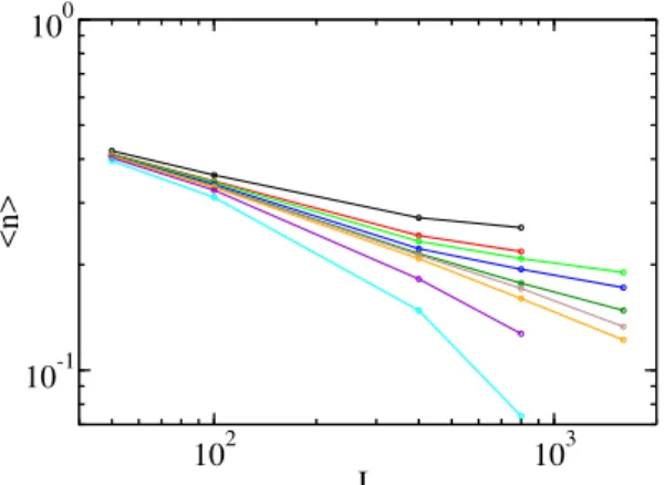
First, we take up the case of a simple (non-attractive) wall, corresponding to b > 0 in Eqs. (1) and (2). Fig. (1) shows how the steady order parameterhnichanges with the system sizeL. Within the active phase, it saturates to a constant value, while in the absorbing one it bends down and decays exponentially. Our best estimate for the crit-ical point is ac = 1.57433(2) and from the slope of the
curve we getβn/ν⊥ ≈0.33(2)[23]. This value ofac
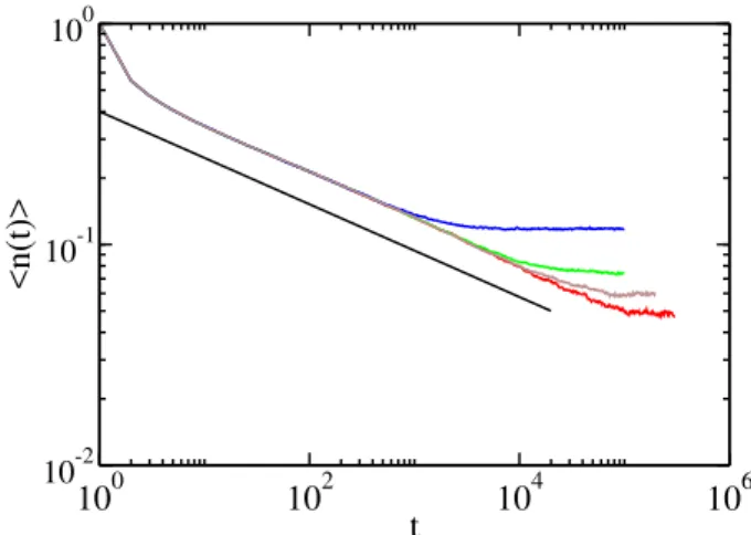
corre-sponds to the point where a free interface (far from the wall) has zero average velocity. The time evolution ofhniat the critical point for different system sizes (Fig. (2)) behaves likehn(t)i ∼ t−θn
, withθn = 0.215(15)or, equivalently,
hh(t)i ∼ tθh, withθ
h = 0.355(15). As for the exponents
β, which govern the saturation of the order parameter within
the active phase, they have been computed using the largest available system sizes (L= 1600and3200). The best fit to
hXi ∼ |a−ac|±βX yieldsβn ≈0.32(3)(forhni) the and
βh = 0.52(2)(for hhi), respectively. The error margin is
typically larger here than for other exponents due to the sen-sitivity to the uncertainty in the determination of the critical point.
102 103
L 10-2
10-1
<n>
Figure 1. Model 1: steady-state values of the order pa-rameter, hni = hexphi, as function of the system size,
L, for drifts (top to bottom) 1.57450, 1.57440, 1.57435, 1.57433, 1.57430, 1.57425, 1.57420. h·idenotes both spa-tial and temporal averages, as well as averages over indepen-dent runs. The straight line corresponds to the critical point
ac= 1.57433(2)and from its slopeβn/ν⊥≈0.33(2).
100 102 104 106
t 10-2
10-1 100
<n(t)>
Figure 2. Model 1: time evolution of the order parameter,
hn(t)i, at criticality,a=ac, for system sizes 100, 400, 800,
and 1600. The saturation values are those of Fig. 1. The best fit givesθn = 0.215(15). The straight line is a guide
for the eye and has a slope -0.215.
It was proved in [6, 7] that these exponents must sat-isfy the scaling relationz = β/(ν⊥θ), wherez is the
dy-namic exponent of the KPZ equation. The exact value for
z in d = 1 is 3/2, thereby z = 0.33/0.215 = 1.5(1)
(βn/ν⊥)/βn = 0.33/0.32, implyingν⊥ ≈ 1. In terms of
hand assumingν⊥ = 1,z = 0.52/.355 = 1.5(1)which,
again, is compatible with3/2within error bars.
The two alternative, but equivalent, mathematical de-scriptions of the MN2 class in terms ofhandn= exp(−h)
can be related noting that the latter is essentially the density of sites at zero hight,n(x, t) =δh(x,t),0[24]. We have
veri-fied thatnandδh(x,t),0exhibit the same asymptotic scaling
behavior.
102 103
L 10-1
100
<n>
Figure 3. Model 1: steady-state values of the order parame-ter for an attractive wall,b=−0.3, as function of the system sizeLfor drifts (top to bottom) 1.57450, 1.57447, 1.57445, 1.57440, 1.57435, 1.57433, 1.57430, 1.57425, 1.57420. The best fit to a straight line again corresponds toac= 1.57433.
Attractive walls can also be simulated within this model by simply replacingabya−bδh,0, whereb <0and the sign
convention is chosen to keep the analogy with Eq. (1). This means that wherever the interface is attached to the wall it experiences an additional (“sticky”) force pushing it against the wall. Extensive Monte Carlo simulations forb =−0.3
show that the previous results, in what respect universal fea-tures, carry over without change, the only difference being that the approach to asymptotics is slower. Upon increasing the attractiveness of the wall the transients become longer. The estimate for the critical point is the same as before (this is due to the fact that the free interface is not affected by variations of the attractiveness parameter). Again, our best estimates for the critical exponents areβn/ν⊥ = 0.32and
θn = 0.215(see Fig. (3)). Forb = −0.4we still observe
a second-order phase transition with a crossover to the men-tioned exponents. For b = −0.5 transition becomes first-order but it still occurs ata =ac. Within the active phase
all the sites are close to the wall and the order parameter is 1, but it suddenly changes to 0 upon decreasinga and hysteresis is observed for slightly subcritical valuesa(the interface is pinned up to long times). Therefore, a tricritical point must exist between0.4 and0.5. We have identified it at b = −0.42(1). The tricritical behavior has not been analyzed.
Let us stress that, contrary to what happens for the MN1 class, where the presence of an attractive wall induces a new and rich phenomenology (including a broad region of
phase coexistence and directed-percolation type transitions [2]), the addition of “attractiveness” has a very mild effect here. Basically, it just shifts the position of the critical point and induces a first-order phase transition for very strong at-tractions.
V.2 Model 2
In order to verify the robustness and eventual universal-ity of the previous results, we have performed a second study of a different model. It is a restricted solid-on-solid (RSOS) model, a variant of the single-step model introduced in [21], in the presence of a wall. A similar model has been recently studied in the context of synchronization transitions [25], to study MN1 type transitions. Initially the wall is located at
hw= 0and a grooved interface is placed beneath it,i.e.the
interface has negative height at all the positions.
The dynamics proceeds as follows: At each time step, a site is randomly picked from a one-dimensional lattice of lengthLand its height decreased two units,h(i)→h(i)−2, provided thath(i)> h(i+ 1)andh(i)> h(i−1),i.e. pro-vided that it is a local maximum. Should the the RSOS con-straint be violated, the trial is discarded and repeated. Every
2(L−1)/[1−2δv(1−L−1)]steps the wall retreats one unit
and, simultaneously, the interface is moved downwards by two units wherever it lies above the wall [25]. The differ-ence between the wall and interface velocities,δv, acts as the control parameter: ifδvis negative, the interface even-tually depins from the wall, while forδv > 0 it remains pinned. It can easily be shown, using random walk argu-ments, that for the chosen wall velocity the system sits at its critical point. By varying it, we have a control parameter. The possibility of computing analytically the critical point largely simplifies the numerical analysis, and makes of this an efficient discrete model.
-7 -6 -5 -4
δv -0,8
-0,6 -0,4 -0,2 0
<e
hw -h >
A
100 102 104 106 t
0,1 1
B
Figure 4. Model 2: (A) order parameter behavior,
hexp(hw−h)i, in the vicinity of the critical pointδvc= 0.
From the slope of the line we getβn= 0.325(5). (B) Decay
of the order parameter,hexp(hw−h)i, at the critical point
yieldsθn = 0.215(5)(cf. with Fig. (2). The straight line is
a guide for the eye and has a slope−0.215.
The quantities monitored arehexp(hw−h)iandhw−h.
We have measured the exponentsβn andθn for a system
ofL = 220sites. Our results lead toβ
n = 0.325(5)and
1 (Fig. (4)). Once more, assumingν⊥ = 1, we getz≈1.51
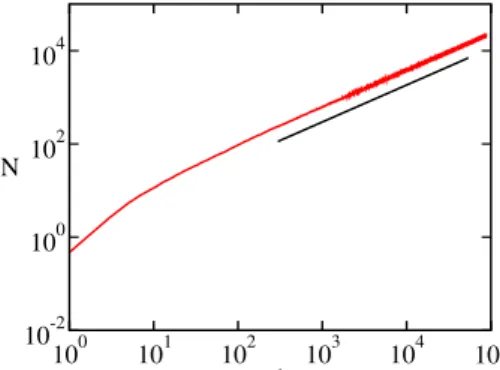
in good agreement with the scaling laws. In addition, we have also measured the spreading exponent,η, that charac-terizes the number of pinned sites. It is computed averag-ing over all the runs and startaverag-ing with an initial condition with a single point attached to the wall. Our best estimate is
η = 0.80(2)(Fig. (5)). Measuring the survival probability, and therefore the exponentsδandζ′
, is a delicate technical point because it is hard to decide when the activity of a run has ceased. We have not tackled this problem here. Lastly, we obtainθh = 0.34(5), which is again in good agreement
with the value reported for our Model 1.
100 101 102 103 104 105 t
10-2 100 102 104
N
Figure 5. Model 2: number of pinned sites as a function of time for an initial condition with a single point attached to the wall. A fit for late times yieldsη= 0.80(2). The straight line is a guide for the eye and has slope0.8.
We have also considered different variations of the model in which the interface can penetrate the wall at some points,i.e. the wall is not perfectly rigid. None of the uni-versal features seem to be affected by this change. In con-clusion, all these results support strongly the existence of robust universality in the MN2 class.
As a matter of consistency, we have modified the algo-rithm of the model to simulate a lower wall, and therefore a case expected to be in the MN1 class. We obtain the set of exponentsβn = 1.69, θn = 1.19andη =−0.4, all of
them in agreement we previously reported results and show-ing that the upper and lower problem belong to different uni-versality classes [2, 7, 9].
V.3 Numerical integration of stochastic
differ-ential equations
As a further test for universality, we have numerically integrated Eq. (1) using Milshtein’s algorithm [26]. A sys-tem size of L = 2000was considered and the time step
and mesh size were set to∆t = 0.001 and∆x = 1, re-spectively. For simulation times up to t = 106 (109
tri-als per site) our results lie far from the asymptotic regime. We do not discard numerical instabilities in the integration scheme, as it is known that results from numerical integra-tions may not agree with the predicintegra-tions from the contin-uum KPZ [27]. The Cole-Hopf transform is a standard way to account numerically for the integration of bounded KPZ equations and, indeed, Langevin equations with MN are by far more stable than their interface-language KPZ-like coun-terparts [7, 9]. Nevertheless, we have also found numerical problems when integrating (2), either when the extra term is written in logarithmic form or averaging for smoothing the gradient. All numerical attempts are unstable nearby the absorbing state, owing to the presence of the extra singu-lar term. We leave, therefore, the numerical integration of a continuous Langevin equation, representative of the MN2 class as an open, challenging problem.
VI
Discussion
We have characterized the MN2 universality class, or analo-gously its bounded KPZ counterpart, which, as commented above, accommodates different physical phenomena. We have studied it from, somehow deceptive mean-field and field theoretical approaches, as well as by numerical stud-ies. None of the analytical methods provides a satisfactory description of the phase transition present in this class. On the other hand, Monte Carlo simulations of two different dis-crete interface models, argued to belong to this universality class, give firm evidence for the existence of a robust univer-sality class. Contrary to what previous simulations seemed to indicate [8], our results are not a simple extension of the ones obtained for one-site, implying that spatial correlations play an important role. Table 1 gathers the values of the critical exponents in terms ofnfor the two discrete models considered in this paper. From the Monte Carlo estimates, it cannot be discarded that they adopt the rational values
βn = 1/3 andθn = 2/9, which combined with the exact
values derived in [6, 7],ν⊥ = 1andz = 3/2, would lead
toβn/ν⊥ = 1/3. Note that our results do not compare well
with those of the nonequilibrium wetting model reported in [11]. We believe this is probably due to the extremely long transients known to be present in that model. We have ver-ified that the transition point is located at the same value of the control parameter for any value of the “attractiveness” parameter (bin Model 1), either representing an attractive or a non attractive wall. For strong enough attractive walls,i.e.
bsufficiently negative, the transition becomes first order as in [11], while if the wall is weakly attractive it remains in the MN2 class.
βn ν⊥ βn/ν⊥ z θn η
Model 1 0.32(2) 0.97(5) 0.34(2) 1.55(5) 0.215(15) not measured Model 2 0.325(5) ≈1 0.33(2) ≈1.5 0.215(5) η = 0.8
The problem of reaching a satisfactory analytical un-derstanding, and even that of obtaining sound results from numerical integrations of the continuous Langevin-equation (in either the interface or the density language) representa-tive of this class remains an open challenge.
Summing up, even though strong evidence is provided confirming the existence of a universality class (i.e. the cor-responding critical exponents are computed with good pre-cision in one dimension and they are universal in two dif-ferent discrete models), its theoretical description in terms of Langevin equations, contrary to what happens for the closely related MN1 class, is far from satisfactory. In par-ticular, the Langevin equation does not seem to admit sound mean-field solutions, nor is it amenable to being treated by means of standard perturbative field theoretical tools, nor does it admit stable numerical integration. Identifying the physical causes at the root of these difficulties is a challenge for future research.
Acknowledgments
F.S. acknowledges financial support from the Fundac¸˜ao para a Ciˆencia e a Tecnologia, contract SFRH/BPD/5654/2001. Financial support from the Spanish MCyT (FEDER) under project BFM2001-2841, and from the AECI, are also acknowledged.
References
[1] See J. Garc´ıa-Ojalvo, and J. M. Sancho,Noise in Spatially Extended Systems, (Springer, New York, 1999); and refer-ences therein. See also, J. M. Sancho and J. Garc´ıa-Ojalvo, in Lecture Notes in Physics557, p.235, edited by J. A. Freund and T. P¨oschel, (Springer-Verlag, Berlin, 2000).
[2] M. A. Mu˜noz, preprint 2003, cond-mat/0303650.
[3] M. Kardar, G. Parisi and Y. C. Zhang, Phys. Rev. Lett.56, 889 (1986).
[4] T. Halpin-Healy and Y.-C. Zhang, Phys. Rep. 254, 215 (1995); and references therein.
[5] A. L. Barab´asi, H. E. Stanley,Fractal Concepts in Surface Growth(Cambridge University Press, Cambridge, 1995); and references therein.
[6] G. Grinstein, M.A. Mu˜noz, and Y. Tu Phys. Rev. Lett.76, 4376 (1996).
[7] Y. Tu, G. Grinstein and M.A. Mu˜noz, Phys. Rev. Lett.78, 274 (1997).
[8] M.A. Mu˜noz and T. Hwa, Europhys. Lett.41, 147 (1998).
[9] W. Genovese and M.A. Mu˜noz, Phys. Rev. E60, 69 (1999).
[10] H. Hinrichsen, R. Livi, D. Mukamel, and A. Politi, Phys. Rev. Lett.79, 2710 (1997).
[11] H. Hinrichsen, R. Livi, D. Mukamel, and A. Politi, Phys. Rev. E61, R1032 (2000).
[12] F. de los Santos, M. M. Telo da Gama, and M. A. Mu ˜noz, Eu-rophys. Lett.57, 803 (2002); Phys. Rev. E67, 021607 (2003); Proceedings of the 7th Granada Seminar on Computational Physics.edited by J. Marro and P. L. Garrido; (American In-stitute of Physics, 2003), p 661; Cond-mat/0211124.
[13] M. A. Mu˜noz and R. Pastor Satorras, Phys. Rev. Lett.90, 204101 (2003).
[14] T. Hwa and M. Lassig, Phys. Rev. Lett.76, 2591 (1996). See also, T. Hwa and M. Lassig, “Optimal Detection of Sequence Similarity by Local Alignment” inProceedings of the Second Annual Int. Conf. on Computational Molecular Biology (RE-COMB98),edited by S. Istrail, P. Pevzner, and M.S. Water-man, 109-116 (ACM Press, 1998) and references therein; R. Olsen, T. Hwa and M. Lassig, “Optimizing Smith-Waterman Alignments” in Pacific Symposium on Biocomputing 4, 302-313 (1999).
[15] R. Lipowsky and M.E. Fisher, Phys. Rev. B36, 2126 (1987).
[16] The sole difference between utilizing the Ito or the Stratonovich conventions, in this case, is a trivial shift ina
[17, 18].
[17] N. G. van Kampen, Stochastic Processes in Physics and Chemistry, (North Holland, Amsterdam, 1981).
[18] C. W. Gardiner,Handbook of Stochastic Methods, (Springer Verlag, Berlin and Heidelberg, 1985).
[19] R. Lipowsky, J. Phys. A18, L585 (1985).
[20] H. D. Fogedby, Phys. Rev. E.57, 4943 (1998). H. D. Fogedby, Cond-mat/0303632.
[21] J. Krug, Adv. in Phys.46, 139 (1997). J. Krug and H. Spohn, inSolids far from equilibrium, edited by C. Godr`eche, (Cam-bridge University Press, Cam(Cam-bridge, 1991).
[22] Observe that the presence of the function “min” in the sec-ond step of the algorithm induces a negative average velocity, implying that in the continuum counterpartλhas to be nega-tive. On the other hand the last stepminh(x, t),0obviously generates an upper wall.
[23] We use the subscriptnto denote exponents related to the or-der parameternandhfor exponents associated with the
av-erage height.
[24] H. Hinrichsen, cond-mat/0302381.
[25] V. Ahlers and A. Pikovsky,
Phys. Rev. Lett. 88, 254101 (2002). V. Ahlers, Ph. D. the-sis. http://www.stat.physik.uni-potsdam.de/volker/publ.html. F. Ginelliet al., cond-mat/0302588.
[26] M. San Miguel and R. Toral, Stochastic Effects in Physi-cal Systems, inInstabilities and Nonequilibrium Structures, VI, edited by E. Tirapegui and W. Zeller, (Kluwer Academic Pub., 1997). (Cond-mat/9707147).