Non-Linear Dynamic Deformation of a Piezothermoelastic Laminate with Feedback Control System

Non-Linear Dynamic Deformation of a Piezothermoelastic

Laminate with Feedback Control System

Masayuki Ishihara*, Tetsuya Mizutani**, and Yoshihiro Ootao***

*(Graduate School of Engineering, Osaka Prefecture University, Japan)

**(Graduate School of Engineering, Osaka Prefecture University, Japan; Currently, Chugai Ro Co., Ltd.,Japan) ***(Graduate School of Engineering, Osaka Prefecture University, Japan)

ABSTRACT

We study the control of free vibration with large amplitude in a piezothermoelastic laminated beam subjected to a uniform temperature with a feedback control system. The analytical model is the symmetrically cross-ply laminated beam composed of the elastic and piezoelectric layers. On the basis of the von Kármán strain and the classical laminate theory, the governing equations for the dynamic behavior are derived. The dynamic behavior is detected by the electric current in the sensor layer through the direct piezoelectric effect. The electric voltage with the magnitude of the current multiplied by the gain is applied to the actuator layer to constitute a feedback control system. The governing equations are reduced by the Galerkin method to a Liénard equation with respect to the representative deflection, and the equation is found to be dependent on the gain and the configuration of the actuator. By introducing the Liénard's phase plane, the equation is analyzed geometrically, and the essential characteristics of the beam and stabilization of the dynamic deformation are demonstrated.

Keywords- feedback control, Liénard equation, piezothermoelastic laminate, vibration, von Kármán strain

I.

INTRODUCTION

Piezoelectric materials have been extensively used as

sensors and actuators to control structural

configuration and to suppress undesired vibration owing to their superior coupling effect between elastic and electric fields. Fiber reinforced plastics (FRPs) such as graphite/epoxy are in demand for constructing lightweight structures because they are lighter than most metals and have high specific strength. Structures composed of laminated FRP and

piezoelectric materials are often called

piezothermoelastic laminates and have attracted considerable attention in fields such as aerospace engineering and micro electro-mechanical systems. For aerospace applications, structures must be comparatively large and lightweight. Because of this, they are vulnerable to disturbances such as environmental temperature changes and collisions with space debris. As a result, deformations due to these disturbances can be relatively large. Therefore, large deformations of piezothermoelastic laminates have been analyzed by several researchers [1-3]. The studies mentioned above [1-3] dealt with the static behavior of piezothermoelastic laminates. However, aerospace applications of these laminates involve dynamic deformation. Therefore, dynamic

problems involving large deformations of

piezothermoelastic laminates have become the focus of several studies [4-7]. In these studies [4-7], the dynamic behavior in the vicinity of the equilibrium state was analyzed. Dynamic deformation deviating arbitrarily from the equilibrium state is very important

from a practical viewpoint for aerospace applications. Therefore, Ishihara et al. analyzed vibration deviating arbitrarily from the equilibrium state and obtained the relationship between the deflection of the laminate and its velocity under various loading conditions [8-10]. In these studies [8-10], methods to suppress undesired vibration due to known mechanical and thermal environmental causes were investigated; in other words, the manner of actuating, rather than the manner of sensing, was investigated.

In order to effectively suppress undesired vibration, it is important to consider both actuation and sensing and to integrate them into a feedback control system. Therefore, Ishihara et al. studied the control of the vibration of a piezothermoelastic laminate with a feedback control system under the framework of infinitesimal deformation [11-13]. However, as mentioned above, large deformation should be considered for applications of piezothermoelastic laminates.

In this study, therefore, we treat the control of the

vibration with large amplitudes in a

piezothermoelastic laminate with a feedback control system. The analytical model is a symmetric cross-ply laminated beam composed of fiber-reinforced laminae and two piezoelectric layers. The beam is simply supported at both edges, and it is exposed to a thermal environment. The undesired vibration of the laminate is transformed into electric current by the direct piezoelectric effect in one of the piezoelectric layers, which serves as a sensor. Then, in order to suppress the vibration, the electric voltage, with the

magnitude of the current multiplied by a gain, is applied to the other piezoelectric layer which is at the opposite side of the sensor and serves as an actuator. Large nonlinear deformation of the beam is analyzed on the basis of the von Kármán strain [14] and classical laminate theory. Equations of motion for the beam are derived using the Galerkin method [15]. Consequently, the dynamic deflection of the beam is found to be governed by a Liénard equation [16], which features a symmetric cubic restoring force and an unsymmetric quadratic damping force due to the geometric nonlinearity. The equation is geometrically studied in order to reveal the essential characteristics of the beam and to investigate how to stabilize the dynamic deformation.

II.

THEORETICAL ANALYSIS

2.1 Problem

y

x

z 2 h



2 h



2 b



2 b

 o a

:

2 /

0 h

z 

2 / h zN 

:

i

z

1

z

: :

:

i

1

N

0

1



i

z

1



N

z



  s1



a N k

k

s k

1

 i N

Fig. 1: analytical model

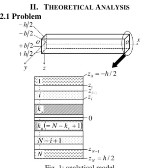
The model under consideration is a simply supported

beam of dimensions abh and composed of N

layers, as shown in Fig. 1. The ks -th and ka-th

layers (

s

s k

k z z

z _1  ,

a

a k

k z z

z _1  ) exhibit

piezoelectricity (with poling in the z or z

direction), while the other layers do not. The beam is laminated in a symmetrical cross-ply manner.

The beam is subjected to temperature distributions

 

xt

T₀ , and T_N

 

x,t on the upper



zh 2



and lower



zh 2



surfaces, respectively, as thermal disturbances that may vary with time t. Mechanical disturbance is modeled as the combination of the initial deflection and velocity.

To suppress the dynamic deformation due to the disturbances, the beam is subjected to the feedback control procedure: electric current Q_s

 

t is detected in the ks-th layer, which serves as a sensor to detect the

deformation due to the disturbances; electrical

potentials

 

xt

a

k1 ,

 and

 

xt

a

k ,

 determined on the

basis of Q_s

 

t are applied to the upper



zzka1



and

lower





a

k

z

z surfaces, respectively, of the ka -th

layer, which serves as an actuator to suppress the deformation due to the disturbances. Moreover, in order to suppress the deformation effectively, the sensor and actuator are designed as a distributed sensor and actuator [17], i.e., the width of the electrodes for the k_s and k_a-th layers are variable as

 

x b f

 

x

bs   s and ba

 

x bfa

 

x , respectively.

2.2 Governing Equations

In this subsection, the fundamental equations which govern the dynamic deformation of the beam are presented.

Based on the classical laminate theory, the

displacements in the x and z directions are

expressed, respectively, as

 

 

w w

 

x t

x t x w z t x u

u 0 , , , _ ,

  

 , (1)

where u0

 

x,t

and w

 

x,t denote the displacements on the central plane



z0



. In order to treat nonlinear deformation, the von Kármán strain is introduced for the normal strain in the x direction as

2 2 2 0

2

2 1 2

1

x w z x w x

u x w x

u

xx _

                         

 . (2)

The electric field in the z direction is expressed by the electric potential





x,z,t



as

z E_z

  

  . (3)

Assuming xx , Dz , and T denote the normal

stress in thex direction, the electric displacement in

the z direction, and the temperature distribution,

respectively, the constitutive equations for each layer are given as

 

xeE T P

Ei xx i i z i

xx







   , (4)

 

xe E P

 

x pT P

Dz i i



xx



i z i i , (5)

where Ei , i , ei , i , and pi denote the elastic

modulus, permittivity, piezoelectric constant, stress-temperature coefficient, and pyroelectric constant, respectively, in the

i

-th layer, and

 





_

  

 

  



s a

i i

k k k

k

k i k i p e

p p e

e

a s a

s

and 0

, 0

, 0 ,

0

. (6)

The function Pi

 

x takes values of +1 and -1 in the

portions with poling in the z and z directions, respectively.

                                   E x T x x E x T x x M M x w D M N N x w x u A N 2 2 2 0 , 2 1

, (7)

where Nx and Mx denote the resultant force and

moment, respectively, defined by







_

_2

 

2 1, d

, h

h xx x

x M z z

N  . (8)

T x

N and T

x

M denote the thermally induced resultant

force and moment, respectively, per unit width defined by





_{ }

 

   N i z z i T x T x i i z z T M N 1 1 d , 1

,  . (9)

E x

N and MxE denote the electrically induced resultant

force and moment, respectively, per unit width. By considering bs

 

x bfs

 

x and ba

 

x bfa

 

x ,

E x

N and MxE are, respectively, defined by

 

 

 

 

   





   





 

 

 

 

   





   





_                               

















        s k s k s s a k a k a a s k s k s s a k a k a a s k s k s s a k a k a a s k s k s s a k a k a a z z z k s k z z z k a k z z s z k k z z a z k k E x z z z k s k z z z k a k z z s z k k z z a z k k E x z z E e x f x P z z E e x f x P z b x b z E e x P z b x b z E e x P M z E e x f x P z E e x f x P z b x b E e x P z b x b E e x P N 1 1 1 1 1 1 1 1 d d d d , d d d d

. (10)

From (10), it is found that P_k

   

x f_a x

a and

   

x f x P_{k a}

a , namely the profiles of poling directions

and widths of the electrodes, determine the effective contribution of the electric field to the electrically

induced resultant force and moment. A and D

denote the extensional and bending rigidities, respectively, defined by

 

_

 

   N i z z i i i z z E D A 1 2 1 d , 1

, . (11)

Equations of motion for the laminated beam are given as 2 2 2 2 2 2 , 0 t w h x w N x M x N x x x           

_

, (12)

where



is defined by

 

_   N i z z i i i z h 1 1

d 1 _

 , (13)

and denotes the mass density averaged along the thickness direction.

By substituting (7) into (12), we have the equations

which govern displacements u0 and w as















 



                        2 2 2 2 0 2 2 2 0 1 , , , x w N N M M x w u L t w h N N x w u L E x T x E x T x E x T x

 , (14)

where the definitions of differentiation operators L1

and L2 are given as

 

 

_                                              4 4 2 2 2 0 0 2 2 2 2 0 2 0 1 2 1 , , , x w D x w x w x u A w u L x w x w x u A w u L . (15)

Because the beam is simply supported at both edges, the mechanical boundary conditions are expressed as

a x M w

u0_0, _0, _x0; _0,

. (16)

The thermally induced resultant force and moment,

T x

N and T

x

M , and the electrically induced resultant

force and moment, E

x

N and E

x

M , must be determined

in order to solve (14). Assuming that the thickness of

the beam h is sufficiently small compared to its

length a, the temperature distribution is considered to be linear with respect to the thickness direction, and it is given as







 

 



 

 





_         t x T t x T h z t x T t x T t z x T N N , , , , 2 1 , , 0 0

. (17)

Substituting (17) into (9) gives

 

 





 

 





_                                   _  





    N i i i i N T x N i i i i N T x h z h z t x T t x T h M h z h z t x T t x T h N 1 3 1 3 0 2 1 1 0 3 1 , , , , , 2 1   .(18)

By assuming the thicknesses of the ks-th and ka-th





 

 

 









 

 

 





                                      a a a a a a a a s s s s s s s s k k k k k k k k k k k k k k k k z z z z z z z t x t x t x t z x z z z z z z z t x t x t x t z x 1 1 1 1 1 1 1 1 1 1 : , , , , , ; : , , , , ,        

. (19)

By substituting (3), (6), and (19) into (10), we have

   







 

 



   







 

 



   





 

 





   





 

 





                                  2 , , 2 , , , , , , , 1 1 1 1 1 1 s s s s s a a a a a s s s a a a k k k k k s s k k k k k a a E x k k k s s k k k a a E x z z t x t x e x f x P z z t x t x e x f x P M t x t x e x f x P t x t x e x f x P N        

, (20)

where

a

k

P and

s

k

P are rewritten as P_a and P_s , respectively, for brevity.

In summary, (14) combined with (18) and (20) and the boundary conditions expressed by (16) are the equations that govern u0 and w, that is, the dynamic deformation of the beam. Note that the applied

electric potentials

 

xt

a

k1 ,

 and

 

xt

a

k ,

 are

determined on the basis of the electric current Q_s

 

t .

 

t

Q_s reflects the dynamic deformation of the beam, and the manner in which Q_s

 

t reflects this dynamic deformation is explained in the following subsection.

The procedures to determine

 

xt

a

k1 ,

 and

 

xt

a

k ,



are provided in Subsection 2.5.

2.3 Sensor Equation

The detected electric current Q_s

 

t is related to the dynamic deformation of the beam through the direct piezoelectric effect of the sensor layer. By considering bs

 

x bfs

 

x , the electric charge Qs

 

t

is evaluated by

 

 

 

 

 

_           _ 





   x x f b D x x f b D t Q a s z z z a s z z z s s k s k d d 2 1 0 0 1

. (21)

By substituting (2), (3), (5), (17), and (19) into (21), differentiating the result with respect to t , and

applying the virtual short condition

 

x t

 

x t

s

s k

k , 



1 ,



, (22)

we have

 

 

 





 

 





   

                      _                     



x x f x bP t x T t x T h z z t x T t x T p x w z z x w x w x u e t Q s s N k k N k

a _{k k}

k s s s s s s s d , , 2 , , 2 1 2 0 1 0 0 2 2 1 0         .(23)

It should be noted that Q_s

 

t can be detected under the virtual short condition of (22) by a current amplifier [17], for example. Thus, the detected electric current Q_s

 

t is related to the dynamic deformation of the beam.

2.4 Galerkin Method

The Galerkin method [15] is used to solve (14) under the condition described by (16) because (15) is a set

of simultaneous nonlinear partial differential

equations. Trigonometric functions are chosen as the trial functions to satisfy (16), and the considered displacements are expressed as the series

 

_





   



  1 0 sin , , m m m

mt w t x u

w

u  , (24)

where

a m

m



  . (25)

Then, the Galerkin method is applied to (14) to obtain





















                                      _     





, ... , 2 , 1 : 0 d sin , , 0 d sin , 2 2 0 2 2 0 2 2 2 0 0 1 m x x x w N N M M x w u L t w h x x N N x w u L m E x T x a E x T x a m E x T x   

. (26)

Moreover, the distributions of temperature on both surfaces of the beam and those of the electric potential

on both surfaces of the ka-th layer are assumed to be

uniform. Thus, one has

 

 

 

 

 



 

 



 

_

 



 x t t xt t

t T t x T t T t x T a a a

a k k k

k N N     , , , , , , , 1 1 0 0

. (27)

Substituting (22) and (27) into (18) and (20) gives

where

 

 





 

 





               2 , 1 1 0 , 1 0 , a a a a a a a a k k k k k E x k k k E x z z t t e M t t e N    

. (29)

In order to satisfy (16), T x

M and E

x

M are evaluated

by using their Fourier series expansions as





_





 

 



 

1

,

, , sin

, m m E m x T m x E x T

x M M t M t x

M  , (30)

where MT

 

t

m

x, and M

 

t

E m

x, are given as

 

 







_

a





m E x T x E m x T m

x M M x x

a t M t M 0 ,

, , sin d

2

,  . (31)

Moreover, in order to construct a modal actuator [17], the profiles of poling direction and the width of the electrode in the ka-th layer are designed to be

   



P x f x



x

a

m a

a sin . (32)

Then, from (28) and (32), one has

x M M x N N a a m E x E x m E x E

x  ,0sin ,  ,0sin , (33)

from which it is found that the actuator induces the

a

m -th mode. By substituting (28) and (33) into (31), we have

 



 

 



 

 

                                  



  a mm E x E m x N i i i i N T m x M t M m m h z h z t T t T h t M    0 , , 1 3 1 3 0 2 , , 2 , mod 4 3 1

. (34)

By substituting (15), (24), (25), (28), (30), and (33) into (26), the simultaneous nonlinear equations with respect to u_m

 

t and w_m

 

t are obtained as









                                          _









                                , ... , 2 , 1 : 8 1 2 1 4 d d , 0 4 2 1 0 , , 2

1 1 1

, 2 1 1 2 1 , 0 , 2 2 2 2 2 0 , 1 1 2 2 m M M w w w A u w A w N w N D t w h N w w u A a a a a mm E x T m x m m i k

k i m m m ik c k i m m l l m lm m l m m m m m s m E x m m T x m m m mm E x m m i im m i m i m m m                     

, (35)

where the definitions of ij, ijk, s,ijk, and c,ijkl are

given in the previous paper [8]. Moreover, by

eliminating um

 

t from (35), we obtain the

simultaneous nonlinear ordinary differential equations with respect to wm

 

t



m1,2,3,,



as

                                                    





              , ... , 2 , 1 : d d

1 1 1 , 1 , 2 2 2 m p p h w h w h w k h w k h w k h w t h A m m m i k

k i m N ik m m m m A m m m m L m m a  ,(36) where

 









 





 





 





                                      





             a a a a a a mm E x m A m A m T m x m m m l lm m ikl l i m m ik c k i m N ik m m E x l l lm lm m m m m m s m A m m m A m m m T x m m L m L m M t p p M t p p A h k N h t k k N D h t k k                    0 , 2 , 2 1 , 2 3 , 0 , 1 , 2 , , 2 2 , , 2 8 1 , 2 4 , .(37)

Moreover, in order to construct a modal sensor [17], the profiles of poling direction and the width of the electrode in the ks-th layer are designed to be

   



P x f x



x

s

m s

s sin



. (38)

From (23), (24), and (27), we have

 

 

 





 

 









                     _           _         





s s N k k N k m m k k m i m i m i imm c m m m m m k s m m t T t T h z z t T t T a b p w z z w w u a b e t Q s s s s s s s s s s 2 , mod 2 2 1 2 4 2 2 0 1 0 2 1 1 1 , 1                  .(39)

Moreover, um

 

t in (39) is eliminated using (35) to

give

 





 

 





 

 









_                        _                               







s s N k k N k m m k k m i m i m i imm c l i k

k i kil k ikl i l k i l m l E x l m lm l m k s m m t T t T h z z t T t T a b p w z z w w w w N A a b e t Q s s s s s s s s s a a s s 2 , mod 2 2 1 2 4 2 2 4 1 2 0 1 0 2 1 1 1 , 1 1 1

1 0 ,                             

. ... (40)

In order to extract the fundamental physical characteristics of the dynamic behavior of the beam, the most fundamental mode is treated as

 

t x w w

 

t x

u

It should be noted that, from (25) and (41), w1

 

t

denotes the deflection of the beam at its center. In order to control the deformation described by (41), the electrode on the actuator is designed as

1 

a

m . (42)

By considering (35) for m1, one has





                               A N A L p p h w k h w k k h w t h u 1 1 3 1 1 1 1 , 1 1 1 1 , 1 1 1 2 2 2 1 d d , 0

 , (43)

where k₁L, k₁A_{,1 1}, k₁N_{,1 1 1}, p1, and A

p₁ defined by (37) are reduced, using Eqs. (41) and (42), to

 









 





 





 





                       E x A A T x N E x A A T x L L M t p p M t p p A h k N h t k k N D h t k k 0 , 2 1 1 1 1 , 2 1 1 1 4 1 3 1 1 1 , 1 0 , 2 1 1 1 , 1 1 1 , 1 2 1 2 1 1 1 , , 8 1 , 3 8 ,       

. (44)

Because the first mode is treated as in (41), the electrode on the sensor is so designed that

1 

s

m . (45)

Then, from (39) and (41), one has

 

 

 





 

 





                   _             t T t T h z z t T t T a b p w z z w w a b e t Q N k k N k k k k s s s s s s s 0 1 0 1 2 1 1 1 1 2 1 2 2 1 2 4 2 3 1 2             . (46)

2.5 Equation for Feedback Control

In this subsection, we derive the equation to treat the control of the free vibration of the beam exposed to constant and uniform temperature.

We consider that the temperature on the upper and lower surfaces of the beam is constant and uniform as

 

t T

 

t 

TN 0 , (47)

which leads to



x z t





T , , , (48)

from (17), (27), and (47). From (28), (34), (46), and (47), we have

0 , 0 ,  _,    T m x T x e T

x h M M

N  , (49)

 

          1 2 1 1 1 1 2 1 4 2 3 1 2 w z z w w a b e t

Q s s

s

k k k

s  

 _ _

 , (50)

where



  _      _  N i i i i e h z h z 1 1   (51)

represents the stress-temperature coefficient averaged with respect to the thickness direction.

We consider that the electric voltage applied to the

actuator,



 

t

 

t



a

a k

k  1

 , is designed to be

proportional to the electric current detected by the sensor, Q_s

 

t , as

 

t _k

 

t GQ_s

 

t

ka a



   1

 , (52)

where G denotes the gain of the feedback control.

By substituting (29), (44), (49), and (52) into (43) and (50), we have





 

 

_                           _{  }        p s p s p e z t Q e G h w A h h w t Q e h G h D h h w t h   2 1 3 1 4 1 3 1 2 1 2 1 2 1 1 2 2 2 8 3 8 d d         , (53)

 

1

2 1 1 3 1 4 2 w w z a b e t

Qs p p  

       _

 , (54)

where

 

2 2

,

0   1   1 

  

 a a s s

s a k k k k p k k p z z z z z e e e ... (55) and zp denotes the z coordinate of the central plane

of the actuator. The case of z_p 0 is treated for brevity. By introducing the nondimensional quantities as

 

                    G hA ab e A ab h e Q hA I hA A h D t hA h z h w W p p s e p p               8 8 , 8 , 8 8 , 8 , , 4 1 2 2 1 2 4 1 2 1 2 4 1 1  , (56)

(53) and (54) are nondimensionalized, respectively, as

p I W W I

W _{ }

            3 2 2 3 8 d d

, (57)

   d d 3 4 2 1 W W

I p 

  



 _

 . (58)

Thus, from (56)-(58), it is found that the

nondimensional deflection W and the

nondimensional electric current I are governed by

nondimensional parameters



, p



0p12



,

and



, which denote the rigidity reduced by

temperature, position of the actuator, and gain, respectively. By substituting (58) into (57), we have

              _       _  0 d d 3 4 3 8 2 1 d d 3 2 2 W W W W W W p p       

It is found that (59) has a set of equilibrium solutions

0 

W , (60)

for



0 and



 0,

W , (61)

for



0. Solutions described by (60) and (61) are different in nature. In this study, we consider that the temperature is lower than a critical value cr as

cr

 

 , (62)

where cr is defined by

h D

e

 2

1 cr 

 . (63)

From (56), (62), and (63), it is found that the condition described by (62) leads to the condition

0 



, (64)

which makes the linear rigidity in (59) positive. It should be noted that the temperature described by (63) is referred to as the buckling temperature.

In order to extract the governing parameters under (64), nondimensional quantities are introduced as

        

p z

t W x

16 3 , ,

,   

 , (65)

where x, t ,



, and z denote the nondimensional quantities of the deflection, time, gain, and actuator's position, respectively, and x, z, and t are different from the coordinates and the time variable defined in Subsection 2.1. Hereafter, x, z, and t are employed in the sense of (65) for brevity. Then, (59) is nondimensionalized as

 

 

0

d d , d

d

2 2

 

 g x

t x z x f t

x

_

, (66)

where functions f

 

x,z and g

 

x are defined as

 





  

3

2 2 4 ,

9 16

,z x z x z g x x x

x

f     

 . (67)

The equation with the form of (66) is known as Liénard's equation [16]. Particularly, if g

 

x is replaced with a linear function x and f

 

x,z with a symmetric function



x21



, (66) is referred to as van der Pol equation. The cubic term in g

 

x defined by

(67) is derived from the nonlinear term ₂

2 x w Nx _



in

(12) combined with (7). The function f

 

x,z defined

by (67) is unsymmetric with respect to x0 because

the weight of the nonlinear term ₂

2 x w Nx _



in the

left-hand side of (12) is different from that of the

nonlinear term

2

2 1

        x w

in the second and third terms

on the right-hand side of (2). In the context of this research, the first, second, and third terms on the

left-hand side of (66) are the terms of inertia, damping, and restoring force of the system, respectively. From (66) and (67), it is found that (66) has its sole equilibrium solution x0. We call the function

 

x z

f , as the damping characteristic function in the sense that it describes the dependency of the damping

intensity for a deflection x. A numerical example of

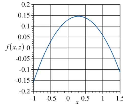
the damping characteristic function f

 

x,z is shown in Fig. 2.

-0.2 -0.15 -0.1 -0.05 0 0.05 0.1 0.15 0.2

-1 -0.5 0 0.5 1 1.5

x

 

x z f ,

Fig. 2: damping characteristic function

Because f

 

x,z is positive in the vicinity of x0, it is found that the equilibrium solution x0 is locally stable for



0. Moreover, from (67) or Fig. 2, it is found that

 

x z z x z

f , 0for2  4 . (68)

Therefore, the equilibrium solution x0 is expected to be not only locally but also globally stable within a

certain range around x0. Conversely, from (67) or

Fig. 2, it is found that

 

x z x z x z

f , 0for 2 or 4 , (69)

which gives the system negative damping for



0. In that case, it is expected that a vibration with relatively large amplitude will be unstable.

Therefore, it is important to determine the range of deformation in which the system is operated stably. For this purpose, the governing equation, (67), is analyzed geometrically by introducing the Liénard's phase plane [18]

 

x,y that is governed by

 



y F x z



y g

 

x x





 , , 1

 

 , (70)

where the overdot denotes differentiation with respect to t, and F

 

x,z is defined by

 

 

     

    

 

 _

     

 

 _

 

 



z x

z x

x

x z x f z x

F x

2 3 105 2

3 105 27

16

d , ,

2 0



. (71)

It should be noted that elimination of y in (70) leads

 

x z F x y  ,





. (72)

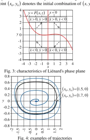
Thus, we call y the modified velocity in the sense that it is related to the actual velocity x. Figure 3 shows the characteristics of the phase plane governed by (70). The solid lines in red denote

 

x z F y

x0,  , , (73)

which make the right-hand sides of (70) null and are, therefore, called nullclines. From (70), it is found that the nullclines in (73) divide the phase plane shown in Fig. 3 into four parts by the signs of x and y. The broken arrows in Fig. 3 denote the directions of the trajectories governed by (70). The examples of the trajectories are indicated by blue lines in Fig. 4. The point



x0,y0



denotes the initial combination of

 

x,y .

-4 -3 -2 -1 0 1 2 3 4

-4 -3 -2 -1 0 1 2 3 4

x y

0



x

 

x z F

y ,

0 ,

0 

 y

x  x0,y0

0 ,

0 

 y

x 

0 ,

0 

 y

x 

Fig. 3: characteristics of Liénard's phase plane

-0.8 -0.6 -0.4 -0.2 0 0.2 0.4 0.6 0.8

-2

-1

.5 -1

-0

.5 0 ₀.5 1 ₁.5 2

x y



x0,y0

 

1.5,0





x0,y0

 

1.7,0



Fig. 4: examples of trajectories

From Fig. 4, it is found that a trajectory may move toward or away from the equilibrium point

   

x,y  0,0 ; in other words, the vibration may be stable or unstable. Therefore, it is expected that there is a closed boundary line that divides the stability as indicated by the broken line in Fig. 4. Such a line is usually called the limit cycle. It should be noted that the limit cycle is numerically obtained by changing the variables as tt in (70) for an arbitrary initial condition and, therefore, is dependent on parameters



and z.

III.

NUMERICAL RESULTS

As stated in Subsection 2.5, the limit cycle divides the stability in the phase plane. In other words, the trajectories that start inside the cycle lead to the sole equilibrium point

   

x,y  0,0 . Therefore, it is important to investigate the shape of the limit cycle. In this section, the effects of parameters



and z on the shape of the phase plane are investigated.

3.1 Effect of Gain

In this subsection, the effect of the nondimensional

parameter



, which represents the gain of the

feedback control, is described.

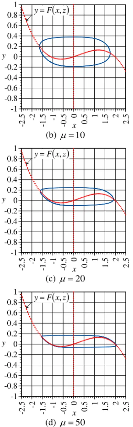
Figures 5 (a)-(d) show the limit cycles for various values of



, in which the blue solid lines and red broken lines denote the limit cycles and the nullclines determined by (73), respectively. In Fig. 5, the limit cycles are found to be horizontal



dy dxy x0



or vertical



dx dyx y0



on the nullclines, which is found also from (70) and (73). Moreover, as shown in Fig. 3, the abscissa or the ordinate of a limit cycle becomes maximum or minimum on the nullclines. From Fig. 5, it is found that, as the value of



increases, the shape of the limit cycle converges to the

shape shown in Fig. 5 (d). This tendency for 1

is explained using (70) as follows. At a point such as

 



yF x,z



~

 

1 , equation (70) implies

 

1

~ 

x and _y ~_

 

1 _1

, which

corresponds to the quasi-horizontal branches of the cycle. In these branches, the trajectory quickly and quasi-horizontally moves to the nullcline yF

 

x,z

because x ~

 

 1 and _y ~

 

1 1 . However, once the trajectory approaches the nullcline so closely that



yF

 

x,z



~

 

2 , then x and y

become comparable as x~

 

1 and y~

 

1 , and the trajectory moves nearly along the nullcline.

-1 -0.8 -0.6 -0.4 -0.2 0 0.2 0.4 0.6 0.8 1

-2

.5 -2

-1

.5 -1

-0

.5 0

0

.5 1

1

.5 2

2

.5

x y

 

xz F

y ,

-1 -0.8 -0.6 -0.4 -0.2 0 0.2 0.4 0.6 0.8 1

-2

.5 -2

-1

.5 -1

-0

.5 0

0

.5 1

1

.5 2

2

.5

x y

 

x z F

y ,

(b)



10

-1 -0.8 -0.6 -0.4 -0.2 0 0.2 0.4 0.6 0.8 1

-2

.5 -2

-1

.5 -1

-0

.5 0

0

.5 1

1

.5 2

2

.5

x y

 

xz F

y ,

(c)



20

-1 -0.8 -0.6 -0.4 -0.2 0 0.2 0.4 0.6 0.8 1

-2

.5 -2

-1

.5 -1

-0

.5 0

0

.5 1

1

.5 2

2

.5

x y

 

x z F

y ,

(d) 50

Fig. 5: effect of gain on limit cycle



z0.3



As x increases, y increases compared with x . Therefore, the trajectory approaches the nullcline and finally crosses the nullcline vertically, as shown in Fig. 3.

The maximum and minimum values of the abscissa and ordinate of a limit cycle are important characteristics of the cycle because they correspond to the limit within which the system is operated safely. To be more precise, the maximum and minimum values of the abscissa correspond to the upper and lower limits of the initial position when the initial

modified velocity is zero, and those of the ordinate correspond to the upper and lower limits of the initial

modified velocity when the initial position is zero. In view of these facts, we refer to the maximum and

minimum values of the abscissa of a limit cycle as the upper and lower limits of the initial position, respectively, and refer to those of the ordinate of the cycle as the upper and lower limits of the initial

modified velocity, respectively. In addition, we refer

to the maximum and minimum values of the actual

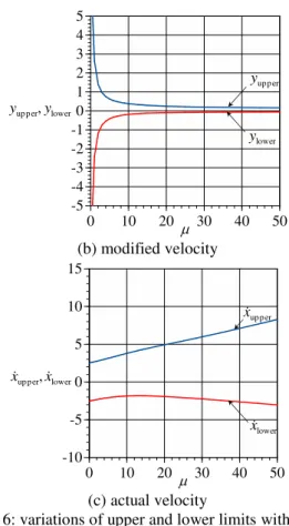
velocity x along the limit cycle as the upper and lower limits of the actual velocity, respectively. Figure 6 shows the variations of the upper and lower limits of the position, modified velocity, and

actual velocity with parameter



, in which subscripts

“upper” and “lower” correspond to the upper and lower limits, respectively. From Figs. 6 (a) and (b), it is found that, as



increases, the upper and lower limits of the position and modified velocity change monotonically and converge to certain values as explained previously. From Fig. 6 (c), it is found that the upper limit of the actual velocity increases as



increases and that the lower limit has a local maximum.

Usually, a larger value of



is preferable in order to quickly pull the system back to the equilibrium point

   

x,y  0,0 . However, as shown in xlo wer in

Fig. 6 (a), the limit within which the system is operated safely may decrease. In this regard, the safe ranges of the initial position xin itial, modified velocity

in itial

y , and actual velocity x_{in itial} are investigated. From Fig. 6, it is found that the system is stable for an arbitrary value of



when xin itial, yin itial, and xin itial

satisfies



1



_{initial upper}



0



lower x x 

x , (74)



1



_{initial upper}



1



lower y y 

y , (75)

and



13



initial upper



0



lower x x 

x   , (76)

respectively.

-2 -1.5 -1 -0.5 0 0.5 1 1.5 2 2.5

0 10 20 _ 30 40 50

lower upper,x

x

up p er

x

lower

x

-5 -4 -3 -2 -1 0 1 2 3 4 5

0 10 20 _ 30 40 50

lower upper,y

y

up p er

y

lower

y

(b) modified velocity

-10 -5 0 5 10 15

0 10 20 _ 30 40 50

lower upper,x

x 

up p er

x

lower

x

(c) actual velocity

Fig. 6: variations of upper and lower limits with gain



z0.3



3.2 Effect of Actuator Position

In this subsection, the effect of the nondimensional

parameter z, which represents the actuator position in

the laminated beam, is described.

-1 -0.8 -0.6 -0.4 -0.2 0 0.2 0.4 0.6 0.8 1

-2

-1

.5 -1

-0

.5 0

0

.5 1

1

.5 2

x y

 

xz F

y ,

(a) z0.1

-1 -0.8 -0.6 -0.4 -0.2 0 0.2 0.4 0.6 0.8 1

-2

-1

.5 -1

-0

.5 0

0

.5 1

1

.5 2

x y

 

xz F

y ,

(b) z0.3

-2 -1.5 -1 -0.5 0 0.5 1 1.5 2

-4 -3 -2 -1 0 1 2 3 4

x y

 

x z F

y ,

(c) z0.5

-4 -2 0 2 4 6 8

-12 -8 -4 0 4 8 12

x y

 

x z F

y ,

(d) z1

Fig. 7: effect of actuator position on limit cycle





10



-6 -4 -2 0 2 4 6 8

0 0.2 0.4 0.6 0.8 1

z

lower upper,x

x

up p er

x

lower

x

(a) position

-3 -2 -1 0 1 2 3 4 5 6 7

0 0.2 0.4 0.6 0.8 1

z

lower up per,y

y yup p er

lower

y

(b) modified velocity

-30 -20 -10 0 10 20 30 40 50 60 70

0 0.2 0.4 0.6 0.8 1

z

lower upper,x

x 

up p er

x

lower

x

(c) actual velocity

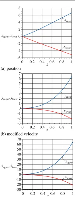
Fig. 8: variations of upper and lower limits with actuator position



z0.3



From Figs. 7 and 8, it is found that the range in which the system is operated safely becomes wider as z

increases. This is explained as follows. From (55),

(56), and (65), parameter z corresponds to the

actuator position in the laminated beam. From (28) and (29), it is found that, the farther out the actuator is installed, the greater the electrically induced resultant moment becomes.

IV.

CONCLUSION

In this study, we treated the control of the free vibration with large amplitude in a piezothermoelastic laminated beam subjected to a uniform temperature with a feedback control system. On the basis of the von Kármán strain, classical laminate theory, and the Galerkin method, the beam was found to be governed by a Liénard equation dependent on the gain of the

feedback control and the configuration of the actuator. By introducing the Liénard's phase plane, the equation was analyzed geometrically, and the essential characteristics of the beam and stabilization of the dynamic deformation were clearly demonstrated. The above-mentioned simplification of the Liénard equation is significantly advantageous because the essential dependence of the system behavior on the system parameters is clearly demonstrated. Moreover, the above-mentioned approach is effective for nonlinear problems because their explicit solutions are rather difficult to obtain. However, our approach is not suitable for cases in which coupling among plural modes is involved.

The findings in this study are considered to serve as fundamental guidelines in the design of piezothermoelastic laminate used for lightweight structures vulnerable to large deformation due to mechanical and thermal disturbances.

REFERENCES

[1] A. Mukherjee and A. S. Chaudhuri,

Piezolaminated beams with large

deformations, International Journal of Solids

and Structures, 39(17), 2002, 4567-4582.

[2] H. S. Shen, Postbuckling of shear deformable

laminated plates with piezoelectric actuators

under complex loading conditions,

International Journal of Solids and Structures, 38(44-45), 2001, 7703-7721.

[3] H. S. Shen, Postbuckling of laminated

cylindrical shells with piezoelectric actuators under combined external pressure and heating, International Journal of Solids and Structures, 39(16), 2002, 4271-4289.

[4] H. S. Tzou and Y. Zhou, Dynamics and

control of nonlinear circular plates with

piezoelectric actuators, Journal of Sound and

Vibration, 188(2), 1995, 189-207.

[5] H. S. Tzou and Y. H. Zhou, Nonlinear

piezothermoelasticity and multi-field

actuations, part 2, control of nonlinear

deflection, buckling and dynamics, Journal

of Vibration and Acoustics, 119, 1997, 382-389.

[6] M. Ishihara and N. Noda, Non-linear

dynamic behavior of a piezothermoelastic laminated plate with anisotropic material

properties, Acta Mechanica 166(1-4), 2003,

103-118.

[7] M. Ishihara and N. Noda, Non-linear

dynamic behavior of a piezothermoelastic laminate considering the effect of transverse shear, Journal of Thermal Stresses,

26(11-12), 2003, 1093-1112.

[8] M. Ishihara and N. Noda, Non-linear

laminate, Philosophical Magazine 85(33-35),

2005, 4159-4179.

[9] Y. Watanabe, M. Ishihara, and N. Noda,

Nonlinear transient behavior of a

piezothermoelastic laminated beam

subjected to mechanical, thermal and electrical load, Journal of Solid Mechanics and Materials Engineering, 3(5), 2009, 758-769.

[10] M. Ishihara, Y. Watanabe, and N. Noda,

Non-linear dynamic deformation of a piezothermoelastic laminate, in H. Irschik, M. Krommer, K. Watanabe, and T. Furukawa

(Ed.), Mechanics and model-based control of

smart materials and structures (Wien: Springer-Verlag, 2010) 85-94.

[11] M. Ishihara, N. Noda, and H. Morishita,

Control of dynamic deformation of a piezoelastic beam subjected to mechanical disturbance by using a closed-loop control

system, Journal of Solid Mechanics and

Materials Engineering 1(7), 2007, 864-874.

[12] M. Ishihara, H. Morishita, and N. Noda,

Control of dynamic deformation of a piezothermoelastic beam with a closed-loop

control system subjected to thermal

disturbance, Journal of Thermal Stresses,

30(9), 2007, 875-888.

[13] M. Ishihara, H. Morishita, and N. Noda,

Control of the transient deformation of a piezoelastic beam with a closed-loop control system subjected to mechanical disturbance

considering the effect of damping, Smart

Materials and Structures, 16(5), 2007, 1880-1887.

[14] C. Y. Chia, Nonlinear analysis of plates

(New York: McGraw-Hill, 1980).

[15] C. A. J. Fletcher, Computational Galerkin method (New York: Springer, 1984).

[16] S. H. Strogatz, Nonlinear dynamics and

chaos (Boulder: Westview Press, 2001). [17] C. -K. Lee, Piezoelectric laminates: Theory

and experiments for distributed sensors and actuators, in H. S. Tzou and G. L. Anderson

(Ed.), Intelligent Structural Systems

(Dordrecht: Kluwer Academic Publishers, 1992) 75-168.

[18] N. Minorsky, Nonlinear Oscillations